Land Use Quantile Regression Modeling of Fine Particulate Matter in Australia

Abstract

Small data samples are still a critical challenge for spatial predictions. Land use regression (LUR) is a widely used model for spatial predictions with observations at a limited number of locations. Studies have demonstrated that LUR models can overcome the limitation exhibited by other spatial prediction models which usually require greater spatial densities of observations. However, the prediction accuracy and robustness of LUR models still need to be improved due to the linear regression within the LUR model. To improve LUR models, this study develops a land use quantile regression (LUQR) model for more accurate spatial predictions for small data samples. The LUQR is an integration of the LUR and quantile regression, which both have advantages in predictions with a small data set of samples. In this study, the LUQR model is applied in predicting spatial distributions of annual mean PM${}_{2.5}$concentrations across the Greater Sydney Region, New South Wales, Australia, with observations at 19 valid monitoring stations in 2020. Cross validation shows that the goodness-of-fit can be improved by 25.6–32.1% by LUQR models when compared with LUR, and prediction root mean squared error (RMSE) and mean absolute error (MAE) can be reduced by 10.6–13.4% and 19.4–24.7% by LUQR models, respectively. This study also indicates that LUQR is a more robust model for the spatial prediction with small data samples than LUR. Thus, LUQR has great potentials to be widely applied in spatial issues with a limited number of observations.

1. Introduction

Small data samples have been a critical challenge for the prediction of geographical attributes [1]. The lack of spatial observations usually leads to biased predictions at locations where there are only sparse or even no observations [2]. In the field of spatial prediction, more observations can benefit accurate spatial prediction [3,4]. As such, a certain number of samples or observations are required in models for spatial prediction. For instance, studies demonstrated that sample sizes of 150 data, or at least 100 data, were recommended for fitting reliable variograms of kriging-based spatial prediction [5]. However, in certain cases, it is difficult to collect enough samples for spatial predictions. The cases of small data samples are usually due to several factors. First, historical data usually contain a limited number of samples, such as meteorological observations in the previous century [6]. In addition, it is difficult to collect massive or enough samples for specific and uncommon attributes or for some regions. For instance, the distribution of global in situ monitoring stations of soil moisture is critically unbalanced [7,8]. In the Qinghai–Tibet Plateau, the number of soil moisture monitoring stations is much fewer than the number of required stations across the whole region [9,10]. The last, but not least, case is that there are only a few samples in small areas. For instance, air pollution monitoring stations are usually limited within a city, which leads to difficulty in regional spatial prediction of air pollution [11,12]. While these monitoring stations may be adequate to describe air quality within the city, they do not provide information necessary to assess air quality in the surrounding countryside. To address the above issues of a limited number of observations, more reliable and robust models are required for dealing with small data samples.

Land use regression (LUR) has proven to be an effective model for the spatial prediction of geographical attributes, with observations at a small number of locations [12,13]. The key part of LUR is to create buffers, areas within specific distances to observation locations, to calculate mean or percentage values of explanatory variables to characterize local geographical, environmental, or social conditions instead of using data values at exact locations of observations [12]. LUR models have been widely applied in spatial predictions due to the advantages in effective prediction with a small number of spatial observations and using categorical variables for predictions. The applications and advantages of LUR models have been reviewed in the next section. In recent years, a series of new models have been developed based on LUR to improve prediction capacity, such as dimensionality reduction for explanatory variables [13], spatiotemporal LUR modelling [14] and the integration of LUR and machine learning algorithms [15,16], as reviewed in the next section.

However, it is still a challenge to more accurately predict spatial distributions with small data samples using the above improved LUR models, where most of them are hybrid and complex models, and relatively large datasets are required for modelling. In addition, the robustness of current LUR models fitted by linear regression still needs to be improved. In linear regression, a few biased or outlier observations will have critical impacts on the accuracy and reliability of LUR models. In previous studies, the commonly used approach to deal with outliers in linear regression models is to remove the outlier observations based on a threshold. For instance, if observations are higher than the mean plus 2.5 times of the standard deviation or lower than the mean minus 2.5 times of the standard deviation, the observations will be regarded as outliers and have to be removed [17]. Unfortunately, for small data samples, if a few data are removed using this approach, the data containing important information may be removed, and the spatial coverage of samples will be critically reduced. In practical studies, spatial predictions with small data samples have been increasingly required, especially in regional and local research and management. Therefore, it is necessary to develop robust models for spatial prediction with very small data samples.

This study develops a land use quantile regression (LUQR) model for more accurate and robust spatial prediction of air pollution with observations at a limited number of locations. The LUQR is an integration of LUR model and quantile regression, which can improve the prediction accuracy and robustness of LUR models that usually use linear regression models for prediction. Quantile regression has proven to be a robust model for small data samples and without assumptions of data distributions, due to the estimation with the median and quantiles [18,19,20]. The primary reason for the robustness of quantile regression is that quantiles are used to derive prediction and tolerance intervals without the assumptions of error distributions and variance of data, and they can effectively deal with outliers in response variables [21,22]. In this study, annual mean PM${}_{2.5}$ (particulate matters with a diameter of 2.5 micrometres or less) concentrations have been collected at 19 valid monitoring stations in the Greater Sydney region, New South Wales (NSW), Australia. Correspondingly, potential explanatory variables of land use, population, road network, elevation, and vegetation have been computed for both buffer regions of PM${}_{2.5}$ monitoring stations and grid data across the Greater Sydney region. The explanatory variables used in the study include most of the commonly used variables for PM${}_{2.5}$ predictions in previous studies [23,24,25,26,27]. Cross validation is performed to assess the accuracy improvement in the LUQR model when compared with traditional LUR models using accuracy indicators of goodness-of-fit measured by R${}^2$ and prediction errors measured by root mean squared error (RMSE) and mean absolute error (MAE).

2. Literature Review

LUR has been applied in various fields, such as the spatial prediction of air pollution [28], climate change [29,30], urban heat islands [31], urban vegetation [32], and soil heavy metals [33]. Among these fields, a primary category is to predict urban air pollution, including PM${}_{2.5}$, PM${}_{10}$ (particulate matters with a diameter of 10 micrometres or less), NO${}_x$, CO, SO${}_2$, O${}_3$, black carbon, etc. [28,34,35,36]. In LUR models, the relationship between an air pollutant and potential explanatory variables is estimated using regression models and the mean values or ratios of explanatory variables within a series of buffers of air pollutant monitoring locations. The potential explanatory variables usually consist of land use and land cover, road networks, traffic intensity, population, vegetation coverage, water areas, elevation, etc. [28,34,35,36]. For instance, in the European Study of Cohorts for Air Pollution Effects (ESCAPE, www.escapeproject.eu) project, spatial distributions of PM${}_{2.5}$, PM${}_{10}$, and other particulate matters were predicted using LUR models for 20 European study areas using observations at 20 sites per area [37]. In the LUR models, a set of explanatory variables were collected for modeling, including traffic conditions, population, and land use within each study area [37]. The goodness-of-fit of LUR models measured by the cross-validation R${}^2$ ranges from 35% to 94% in different areas, and the median goodness-of-fit is 71% [37]. In the United States, the satellite remote sensing data aerosol optical depth (AOD) was used to improve the spatial prediction accuracy of PM${}_{2.5}$ [38]. The results show that with the supports of AOD data and random slope in the LUR models, the cross validation R${}^2$ of the spatial prediction can be improved from 0.50 to 0.66 [38].

LUR models have the following advantages in spatial predictions compared with geostatistical models, such as kriging-based models. First, LUR models are effective in spatial predictions with observations at 20–100 locations [28], depending on the required size of observations, which are much lower than the required number of locations in kriging-based spatial prediction models. In general, if the total number of observations is lower than 15 or 20, it is difficult to construct a reliable variogram function in kriging-based models. In practical spatial prediction issues, more observations and hybrid approaches are required in kriging-based models due to the common uneven distributions of samples [39,40]. The uneven distributions of samples are also a critical issue for the air pollution data, including particulate matter, where samples are generally clustered in central urban regions and are sparse in rural and remote areas [38]. If kriging-based models are used for the spatial prediction of particulate matters, the variogram function can only present the spatial characteristics, i.e., patterns and heterogeneity, of particulate matters in central urban areas. This phenomenon will further lead to biased and unreliable prediction in rural areas. However, LUR models can address this issue to some extent through building relationships between particulate matters with local land use, environmental, and social conditions within buffers of certain distance [28].

In addition, LUR models can effectively use categorical variables, such as land use, in models [35,36], which are difficult to be added in kriging-based models. The common categorical variables of geospatial data include land cover and land use, soil types, geological strata, river catchment zones, climate zones, ecological zones, etc. In LUR models, the geographical information of categorical variables can be depicted by comparing response variables with area ratios of different types of data in a categorical variable, e.g., land use, within buffers of multiple distance ranges. In this way, the maximum impacts of a type of categorical data can be estimated.

In recent years, to improve the capacity of LUR models in spatial prediction, a set of innovative models have been developed. For instance, principal component analysis was used to optimize LUR models through the dimensionality reduction for explanatory variables [13]. In addition, a spatiotemporal LUR model was developed to enhance the spatiotemporal estimation of air pollutants even with missing data [14]. The spatiotemporal LUR model was a hybrid two-stage model integrating a static LUR model and a multiple linear-regression-based meteorological factor regression (MFR) model for more accurate spatiotemporal predictions [41]. Finally, an LUR model was integrated with machine learning algorithms to improve the prediction accuracy, where the linear relationships between air pollutants and explanatory variables are replaced by nonlinear relationships explored by machine learning [15,16]. For instance, non-parametric LUR models were developed with the support of a random forest model and a generalized additive model for predicting spatial distributions of ambient total particulate concentrations [42], and additive regression smoother-based LUR models were developed for investigating agglomeration and infrastructure effects on air pollutants [43]. Previous studies also have demonstrated that the accuracy of LUR and improved models-based spatial predictions, such as the prediction of particulate matter, are much higher than kriging-based models, especially for cases with relatively low numbers of observations [24].

3. Study Area and Data

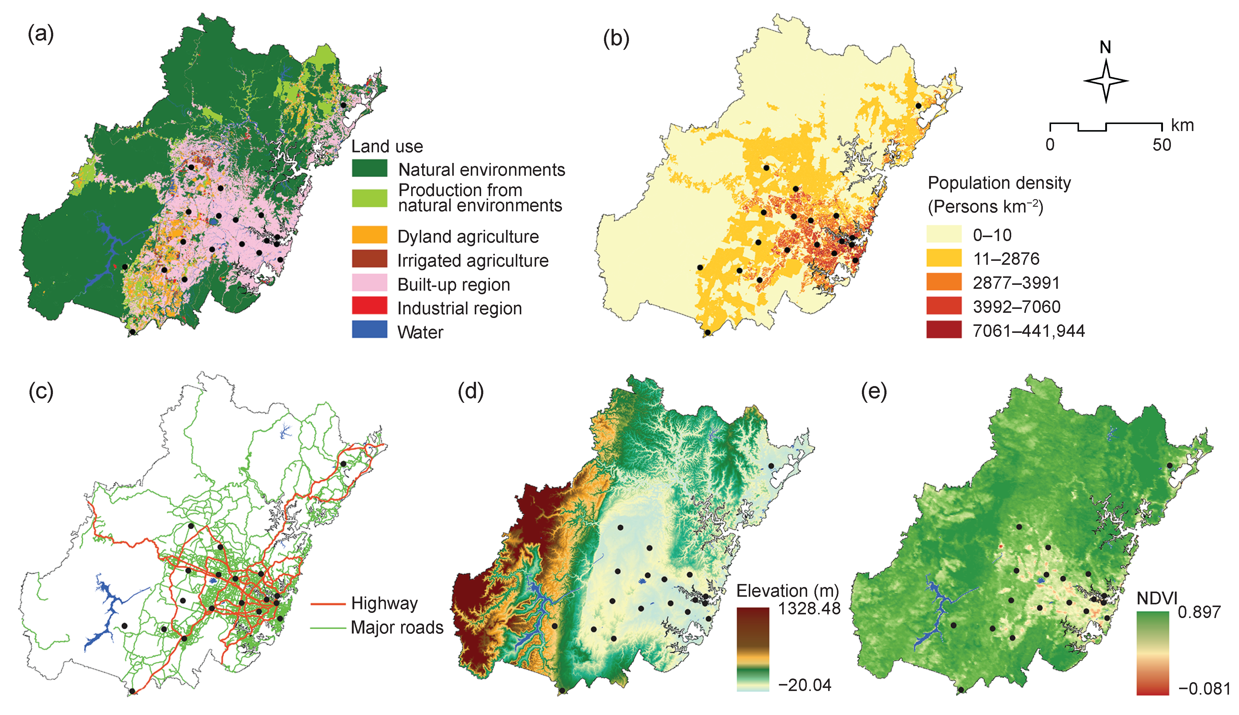
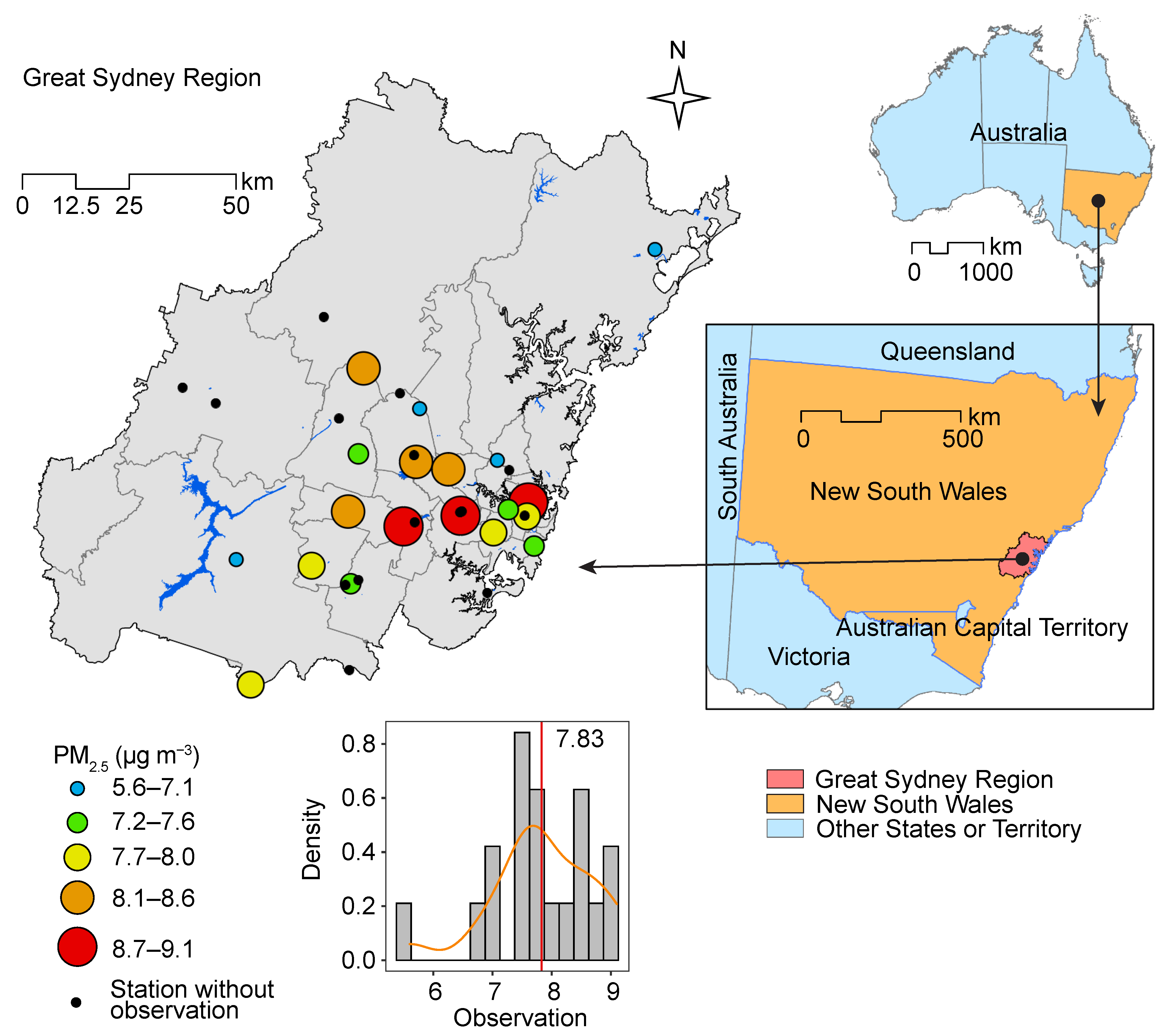
3.1. Study Area and Air Pollution Data

Air pollution monitoring stations are usually unequally distributed in most nations. In general, air pollution monitoring stations are densely distributed in populated urban areas and sparsely distributed in rural and remote areas. The study area is the Greater Sydney Region in New South Wales, Australia. The population in the Greater Sydney Region is 5.31 million, which accounts for about 65.1% of the population of New South Wales and 20.9% of the total Australian population [44]. Similar to most cities in the world, the spatial data of air pollutants are much fewer than the temporal data in the Greater Sydney Region. From the temporal perspective, air pollutant data are updated hourly, and a daily air pollutant forecast is available in the Greater Sydney Region [45]. However, spatial data of air pollutants are limited for predicting distribution maps.

In the Greater Sydney Region, there are 34 monitoring stations for different types of air pollutants, such as PM${}_{2.5}$, PM${}_{10}$, SO${}_2$, NO${}_2$, and O${}_3$ [45]. The number of stations has been continuously increased in recent years to cover more typical areas and improve the capacity to monitor air pollution. The number of PM${}_{2.5}$ monitoring stations has been increased from 15 in 2018 to 19 in 2020. In this study, the annual mean PM${}_{2.5}$ concentrations at the 19 valid stations in 2020 are used to predict the spatial distribution of annual mean concentrations in Greater Sydney Region (Figure 1). PM${}_{2.5}$ is the fine particulates with the size smaller than 2.5 $\mathsf{\mu }$m in aerodynamic diameter [46,47]. PM${}_{2.5}$ is a mixture, and its components are sophisticated and varied in different locations. The potential sources of PM${}_{2.5}$ primarily consist of traffic [48,49,50], industrial activities [51,52], bushfire [53], residential energy use and biomass burning [54,55], and agricultural products and straw burning [56]. The map shows that the general spatial pattern of PM${}_{2.5}$ concentrations is that PM${}_{2.5}$ in urban regions (southeastern regions) tend to be higher than that in rural regions. The distribution pattern and rural–urban difference of PM${}_{2.5}$ indicate that, from the spatial perspective, PM${}_{2.5}$ is closely associated with traffic and other human activities.

Table 1. Particulate matter observations and selected explanatory variables.

Variable		Code	Optimal Buffer (km)	Min	Mean	Median	Max	Std ${}^{\mathit{a}}$
PM${}_{2.5}$ ($\mathsf{\mu }$g/m${}^3$)		/	/	5.60	7.83	7.80	9.10	0.86
Land use: ratio (%)	Natural environments	NE	3	0.38	12.22	6.51	63.19	15.38
	Production from natural environments	PNE	3.5	0.00	3.87	0.56	30.04	7.51
	Dryland agriculture	DA	0.5	0.00	7.86	0.00	45.00	13.18
	Built-up region	BUR	3	16.08	61.81	62.75	78.44	15.62
	Industrial region	IR	3	0.85	14.93	13.37	27.04	8.07
Population density (persons/km${}^2$)		PPDS	5	110	3077	2328	9292	2767
Highway density (km/km${}^2$)		HWDS	2.5	0.000	0.821	0.688	2.600	0.790
Major road density (km/km${}^2$)		MRDS	4.5	0.169	1.710	1.828	3.925	1.093
Elevation (m)		ELV	5	14.04	81.54	45.28	416.71	108.23
NDVI		NDVI	0.5	0.368	0.534	0.533	0.732	0.107

^a Std: Standard deviation.

shows the statistical summary of PM${}_{2.5}$ observations. The concentrations at the 19 stations range from 5.60 to 9.10 $\mathsf{\mu }$g m${}^{-3}$, and the mean value is 7.83 $\mathsf{\mu }$g m${}^{-3}$.

3.2. Explanatory Variables

To predict spatial distributions of PM${}_{2.5}$ concentrations, data of five categories of explanatory variables in 2020 have been collected, including land use types, population, road network distributions, elevation, and vegetation coverage. Figure 2 shows spatial distributions of the five categories of explanatory variables and the relationships between their distribution patterns and valid PM${}_{2.5}$ monitoring stations at the Greater Sydney region. The brief descriptions and data sources of the five categories of explanatory variables are presented as follows.

3.2.1. Land Use

Spatial distributions of PM${}_{2.5}$ are closely associated with land use, such as built-up areas, forest, and rivers [57,58]. As such, land use has been an effective variable for the prediction distributions of PM${}_{2.5}$ [59,60]. Land use data are sourced from the catchment scale land use of Australia (CLUM) [61], which is a 50-m resolution raster data of land use updated on December 2020 and contains 18 major classes of land use. In the study, due to the limited number of PM${}_{2.5}$ monitoring stations, the major classes of land use have been summarized into seven categories in the study area according to the characteristics explained by the CLUM [61]. The summarized land use types used for PM${}_{2.5}$ prediction include natural environments, production from natural environments, dryland agriculture, irrigated agriculture, built-up regions, industrial regions, and water, as shown in Figure 2a. The land use map demonstrates that most of the PM${}_{2.5}$ monitoring stations are located in the urban built-up regions, and a few other stations are distributed in natural environments, production regions from natural environments, and dryland agriculture regions.

3.2.2. Population

The inequality of population distributions between rural and urban areas is also an essential factor of the spatial patterns of PM${}_{2.5}$. The population variable is an effective proxy indicator of human activities, such as motor vehicles, freight transportation, the use of energy, etc., and human-related combustion that is the primary source of PM${}_{2.5}$. In Australia, very high resolution block-level population data are available from the Australian Bureau of Statistics [62], and it is used to calculate the block-level population density in Greater Sydney Region (Figure 2b). The population density map shows significant spatial disparities of population in the study area. The most of the population are densely distributed in central urban regions of Sydney, and sparsely distributed in rural areas. For instance, in rural and remote areas, the population density is generally lower than 10 persons/km${}^2$. However, in the central urban regions, the population densities in most blocks are higher than 2800 persons/km${}^2$, and the highest block-level population density reaches to 441,944 persons/km${}^2$, which is a commercial block area in the central urban region.

3.2.3. Road Network

Road network is a commonly used variable for prediction of air pollutants, since it is closely associated with traffic emissions and other population activities that may release air pollutants, such as household emissions and industry emissions. In this study, the latest road network data in 2020 are sourced from OpenStreetMap (OSM) data. The road network data are reclassified into highways and major roads, where major roads include primary roads, secondary roads, tertiary roads, and their links in the road network of OSM. In the study, the highway represent the primary inter-region passenger and freight transportation. The major roads can support regional and local transportation. For instance, the transport of mines, agricultural products, general manufactures, construction materials, and household consumables between regions and ports in Sydney are essential components of the freight transportation. The map of the road networks show that most of the PM${}_{2.5}$ monitoring stations are located close to highways.

3.2.4. Elevation

The elevation data are used to present the geographical conditions of the study area. The elevation data are sourced from the Digital Elevation Model (DEM) of Australia [63] at Google Earth Engine (GEE) [64]. In the study area, most of the eastern parts are plain regions with relatively low elevation, and the western and northern parts are mountainous areas with high elevation. The highest elevation is about 1328 m. The relationship of spatial distribution patterns between elevation and the PM${}_{2.5}$ monitoring stations shows that most of the monitoring stations are located in the plain regions, and only a few of them are distributed in mountainous regions. This phenomenon also indicates the spatial inequality of the PM${}_{2.5}$ observations.

3.2.5. Vegetation

The vegetation condition is an effective proxy indicator of ecological and environmental conditions, which are liked with spatial distribution patterns of air pollutants. For instance, a series of studies have demonstrated that the vegetation cover and green spaces have impacts on the spatial and temporal variations of PM${}_{2.5}$ concentrations [65,66,67]. In this study, the vegetation condition is presented using the annual mean normalized difference vegetation index (NDVI) derived from the MOD13A1.006 Terra Vegetation Indices [68] at GEE. The map shows that the vegetation coverage is high in most of the study area, and the low vegetation coverage is only distributed in a small area of the central urban region.

To ensure the consistent data analysis from both spatial and temporal perspectives, all the above explanatory data have been transformed to data with a spatial resolution of 100 m and calculated to annual mean values in 2020 for the following LUQR modeling.

4. Land Use Quantile Regression (LUQR) for Air Pollution Prediction

This study proposed an LUQR model, which is an integration of LUR and quantile regression, for the spatial prediction of air pollution. In this study, the LUQR-based model for air pollution prediction includes following six steps.

The first step is to calculate circle buffer values of explanatory variables. Spatial-buffer-based variables are generated for each type of explanatory variable using a series of buffers with radius from 0.5 km to 5 km with an interval of 0.5 km. Ratios of land use types within buffers are calculated for land use variables, which consist of natural environmental land, production land from natural environments, dryland agricultural regions, built-up regions, and industrial regions. Among seven classes of land use, most ratio values of irrigated agricultural lands and water within buffers are zero, which may lead to biased and invalid estimation. Thus, these two classes of land use data are removed. For the continuous explanatory variables, including population density, highway density, major road density, geographical elevation, and NDVI, mean values within buffers are calculated for both locations of air pollution monitoring stations (i.e., observations) and prediction locations.

The next two steps are used for buffer-based variable selection. In general, in LUR models, buffer-based variable selection can be performed in three approaches. The first approach is selecting an optimal buffer for each individual variable and then determining buffer-based variables from these optimal buffer-based variables. The second approach is directly selecting variables from all buffer-based variables. The last approach is ranking all buffer-based variables in terms of their correlation with the dependent variable, identifying the buffer-based variable with the highest correlation with the dependent variable, adding variables based on ranks, and finally determining the optimal combinations of variables. In this study, the first approach is used for buffer-based variable selection, as it is the most used approach in LUR models. The details are introduced in the following two paragraphs.

In the second step, optimal buffers are determined for each explanatory variable using correlation analysis. For a specific explanatory variable, the optimal buffer is the buffer that enables the highest correlation between PM${}_{2.5}$ concentrations and this variable. For the selected five classes of land use and other five explanatory variables, buffers with the highest Pearson correlation coefficients with PM${}_{2.5}$ concentrations are selected as the optimal buffers. As a result, an optimal buffer-based variable is selected for each explanatory variable.

The third step is to select variables for the LUQR model from the above 10 optimal buffer-based variables. Pearson correlation is used to select variables with significant correlation coefficients with PM${}_{2.5}$ concentrations. Then, multicollinearity analysis is performed to remove variables with high collinearity with others according to variance inflation factor (VIF). Variables with all VIF values lower than 4 are selected for following modelling [69,70,71].

The fourth step is to construct an LUQR model using the above selected variables. The LUQR model for predicting spatial distributions of PM${}_{2.5}$ concentrations is calculated as a conditional quantile function:

$$\begin{array}{c}\hfill Q_Y\left(\tau \right|X)=\sum _{j=1}^N{\beta }_j\left(\tau \right)X_{j,b_j}\end{array}$$

(1)

where $Q_Y\left(\tau \right|X)$ is the $\tau$th conditional quantile of the response variable Y [21,22], $X_{j,b_j}$ is the jth ($j=1,\cdots ,N$) explanatory variable with the optimal buffer $b_j$, and ${\beta }_j\left(\tau \right)$ are coefficients of the $\tau$th quantile of explanatory variables. The process of quantile-regression-based parameter estimation includes the following steps. In each quantile, the model is fitted using a linear programming method [72]. When the quantile $\tau$ is set to different values, corresponding estimates of ${\beta }_j\left(\tau \right)$ for different quantiles can be computed. In this study, to effectively present the comprehensive association between dependent and independent variables, all percentiles, i.e., 100 quantiles, are used as quantile points for modelling. This processing is consistent with most studies about quantile regressions and can reflect details of small data sample distributions.

The fifth step is to validate the LUQR model using a leave-one-out cross validation (LOOCV) approach, which is a reasonable model validation method for this case, since there are only 19 locations in the study area. In the LOOCV, the observation at each site location is used as a validation data set, and observations at the remaining 18 locations are considered as the training data set. The LUQR model is constructed using the training data set and used to predict at the validation data site location. The modelling and prediction process is performed 19 times, and prediction accuracy is assessed using the cross-validation indicators explained below. In this study, to ensure consistent comparison, the LUQR model that uses quantile regression for prediction is compared with an LUR model that uses linear regression for prediction, where identical selected explanatory variables are used for modeling. The cross-validation indicators include R${}^2$, RMSE and MAE. The cross-validation indicators are calculated as:

$$\begin{array}{c}\hfill {\mathrm{R}}^2=1-\sum {(Y_i-\widehat{Y})}^2/\sum {(Y_i-\overline{Y})}^2\end{array}$$

(2)

$$\begin{array}{c}\hfill \mathrm{RMSE}=\sqrt{1/n\sum _{i=1}^n{(Y_i-\widehat{Y})}^2}\end{array}$$

(3)

$$\begin{array}{c}\hfill \mathrm{MAE}=1/n\sum _{i=1}^n\left|Y_i-\widehat{Y}\right|\end{array}$$

(4)

where $Y_i$ is the ith ($i=1,\cdots ,n$) observation, $\widehat{Y}$ is predictions, and $\overline{Y}$ is the mean value of observations. Note that the above cross-validation indicators measure the global goodness-of-fit over the entire condition distribution, and they are used to compare modelling accuracy and errors between LUQR and LUR models. If the aim of model evaluation is to assess the goodness-of-fit at a specific quantile of LUQR, it is recommended to use quantile-specified goodness-of-fit mentioned in the page 1297 in [73].

The last step is to predict spatial distributions using the LUQR model estimated in above steps. In this study, to ensure a high-resolution mapping of PM${}_{2.5}$ concentrations, 500 m resolution grid data are generated for all spatial buffer-based explanatory variables in the whole study area. Thus, spatial distributions of PM${}_{2.5}$ concentrations with a 500 m resolution can be predicted using the LUQR model in the Greater Sydney Region.

5. Results

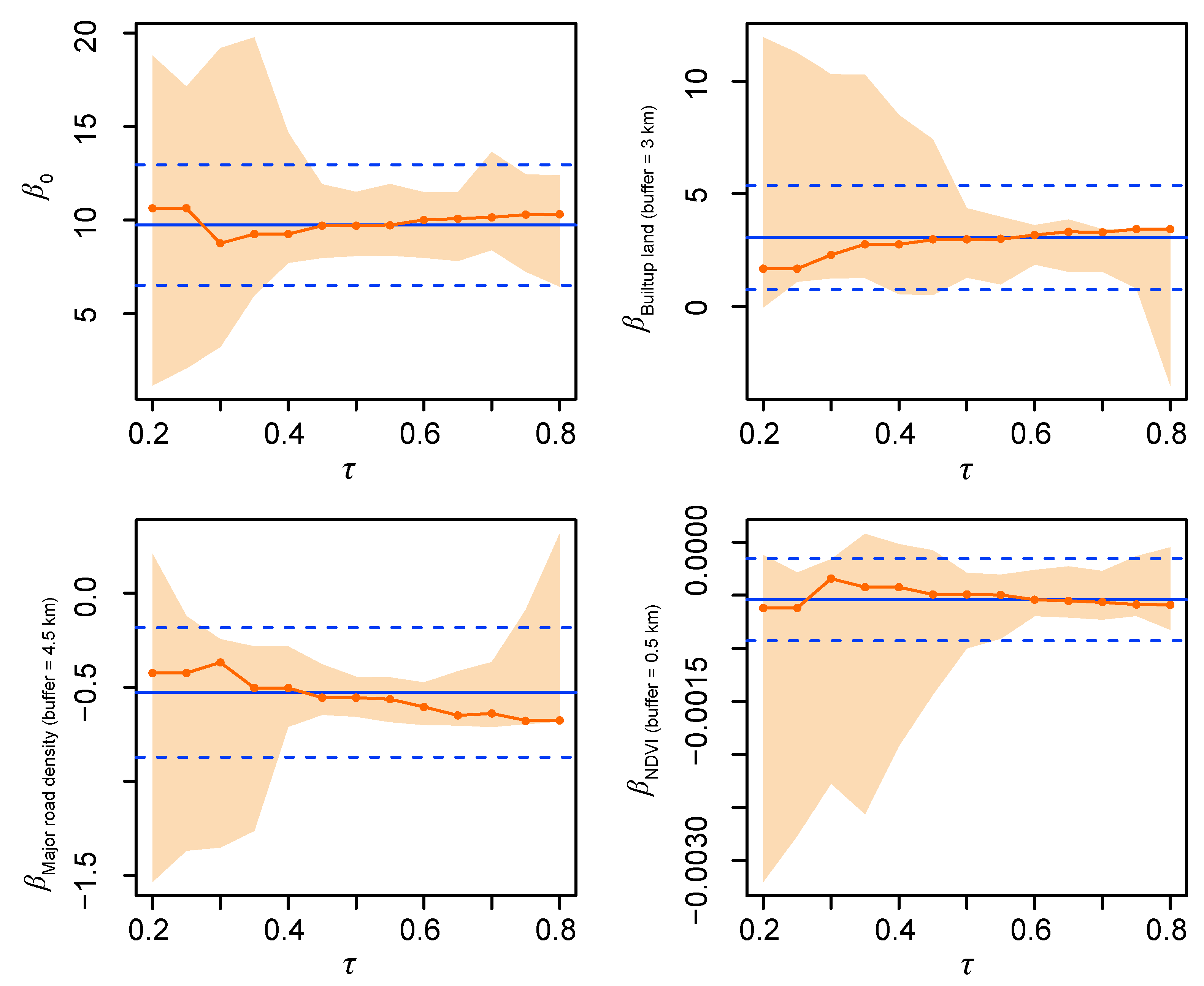
5.1. Optimal Spatial Buffers and Variable Selection

The determined optimal buffers which enable the highest correlation between the response variable and buffer-based explanatory variables are listed in Table 1. A brief statistical summary of 10 potential buffer-based explanatory variables, including 5 types of land use, population density, highway density, major road density, elevation, and NDVI, at the locations of PM${}_{2.5}$ monitoring stations is shown in Table 1.

Furthermore, out of the 10 potential buffer-based variables, 3 are selected through the Pearson correlation analysis and multicollinearity analysis for the LUQR model. The three variables are built-up regions with a 3 km buffer, major road density with a 4.5 km buffer, and NDVI with a 0.5 km buffer.

5.2. LUQR Model

The constructed LUQR model for predicting PM${}_{2.5}$ concentrations using the selected variables is as follows:

$$\begin{array}{c}\hfill Q_Y\left(\tau \right|X)={\beta }_0\left(\tau \right)+{\beta }_1\left(\tau \right)X_{BUR,b=3}+{\beta }_2\left(\tau \right)X_{MRDS,b=4.5}+{\beta }_3\left(\tau \right)X_{NDVI,b=0.5}\end{array}$$

(5)

where $X_{BUR,b=3}$, $X_{MRDS,b=4.5}$, and $X_{NDVI,b=0.5}$ are the built-up regions with a 3 km buffer, major road density with a 4.5 km buffer, and NDVI with a 0.5 km buffer, respectively.

Figure 3 shows the coefficients of the quantiles of the explanatory variables in the LUQR model for PM${}_{2.5}$ prediction. In the LUQR model, the coefficients are varied with $\tau$ values. For instance, coefficients of $X_{BUR,b=3}$ are generally increased with $\tau$ values, but coefficients of $X_{MRDS,b=4.5}$ and $X_{NDVI,b=0.5}$ are generally decreased with $\tau$ values, although such decreases are fluctuating. In addition, in most ranges of $\tau$ values, the CIs of LUQR coefficients (orange areas) are thinner than that of linear regression coefficients (areas between blue dashed lines). This means that in most quantiles of variables, LUQR coefficients are more reliable than linear regression models.

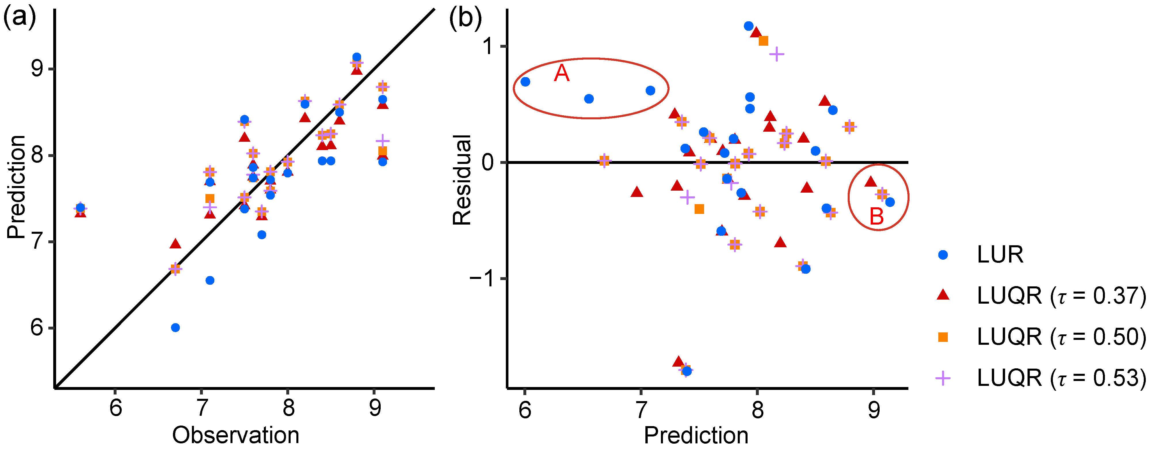
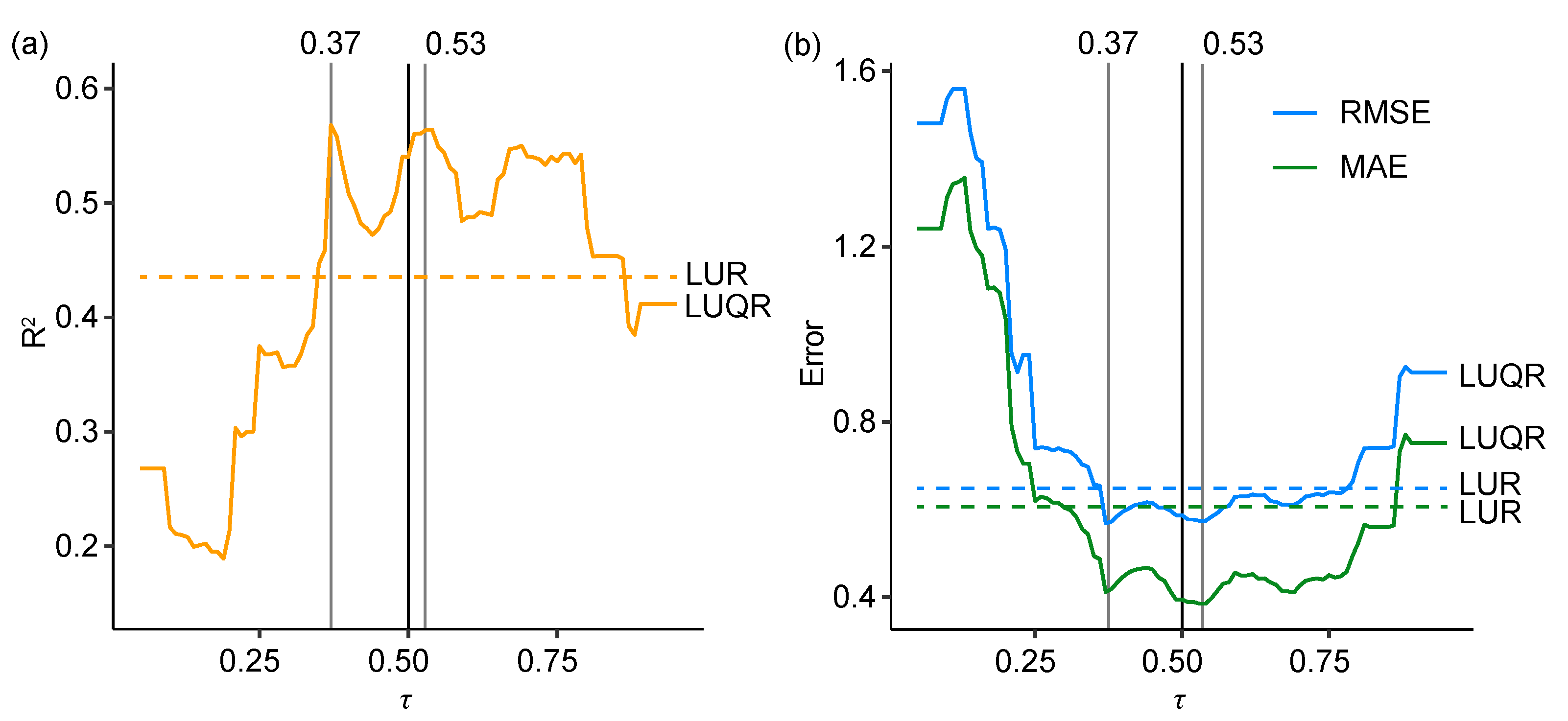
5.3. Model Validation

LOOCV is first performed for each spatial buffer-based explanatory variable as shown in

Table 2. Goodness-of-fit and errors of land use regression (LUR) models for selected individual explanatory variables. The unit of RMSE and MAE is $\mathsf{\mu }$g/m${}^3$.

Variable		Code	Optimal Buffer (km)	R${}^2$	RMSE	MAE
Land use: ratio (%)	Natural environments	NE	3	0.187	0.835	0.706
	Production from natural environments	PNE	3.5	0.001	1.129	0.813
	Dryland agriculture	DA	0.5	0.057	0.894	0.684
	Built-up regions	BUR	3	0.234	0.754	0.638
	Industrial regions	IR	3	0.033	0.902	0.741
Population density (persons/km${}^2$)		PPDS	5	0.002	0.898	0.735
Highway density (km/km${}^2$)		HWDS	2.5	0.053	0.847	0.693
Major road density (km/km${}^2$)		MRDS	4.5	0.037	0.910	0.746
Elevation (m)		ELV	5	0.189	0.765	0.620
NDVI		NDVI	0.5	0.034	0.905	0.708

. Among the 10 buffer-based variables, the built-up region with a 3 km buffer variable has the highest cross-validation R${}^2$ (0.234) and the lowest prediction errors (RMSE = 0.754). The cross-validation R${}^2$ and RMSE values of major road density are 0.189 and 0.765, respectively.

The constructed LUR model for PM${}_{2.5}$ prediction is as follows:

$$\begin{array}{c}\hfill Y=9.733+3.052X_{BUR,b=3}-0.527X_{MRDS,b=4.5}-5.419X_{NDVI,b=0.5}\end{array}$$

(6)

where the explanatory variables were identical with those selected in the LUQR model for consistent comparison.

Figure 4 shows the LOOCV of the LUQR model for PM${}_{2.5}$ prediction with different values of quantile parameter $\tau$. In this study, three $\tau$ values are used to present the accuracy of the LUQR model, including 0.37, 0.50, and 0.53. In most studies of quantile regression, the quantile model of $\tau =0.50$ is usually used to indicate the overall accuracy of LUQR, since $\tau =0.50$ means that the median values of the variables are used for prediction. In this study, another two $\tau$ values, 0.37 and 0.53, which enable the highest LOOCV goodness-of-fit and the lowest errors on the left and right sides of the median value are identified. The analysis also finds that the LOOCV goodness-of-fit of the quantiles when $\tau =0.37$ and $\tau =0.53$ are both higher than the quantile when $\tau =0.50$. This phenomenon may be closely related to the biased sampling and distributions of PM${}_{2.5}$ monitoring stations. Since no assumptions are required for the data distributions in LUQR models, LUQR models can effectively deal with the biased samples for robust modelling. Thus, it also proved that the LUQR model is an effective model to identify different relationships between response and explanatory variables at different quantiles.

Table 3. Model evaluation using a leave-one-out cross validation. The unit of RMSE and MAE is $\mathsf{\mu }$g/m${}^3$.

Model	R${}^2$	RMSE	MAE
LUQR ($\tau$ = 0.37)	0.568	0.569	0.412
LUQR ($\tau$ = 0.50)	0.540	0.587	0.395
LUQR ($\tau$ = 0.53)	0.564	0.574	0.385
LUR	0.430	0.657	0.511

shows a comparison between the LUQR and LUR models using an LOOCV approach. In general, the LUQR model has a higher LOOCV goodness-of-fit than the LUR model and has lower prediction errors than the LUR model. Compared with the LUR model, the goodness-of-fit is improved by 25.6%, and the RMSE and MAE are reduced by 10.6% and 22.7%, respectively, by the LUQR model with $\tau =0.50$. In addition, the LUQR model with $\tau =0.37$ and $\tau =0.53$ can improve the goodness-of-fit of the LUR models by 32.1% and 31.2%, respectively, reduce RMSE by 13.4% and 12.6%, respectively, and reduce MAE by 19.4% and 24.7%, respectively. As R${}^2$ may not have a sensible interpretation in quantile regression [73], prediction error indicators RMSE and MAE can more effectively indicate the accuracy improvement of the LUQR models than R${}^2$. In summary, predictor error indicators RMSE and MAE can be reduced by 10.6–13.4% and 19.4–24.7% by the LUQR models, respectively, compared with the LUR model. Thus, the LUQR model with $\tau =0.37$ is the optimal model among LUQR model with all three quantile parameters.

Figure 5 evaluates LUR and LUQR models through the comparison between observations and predictions of PM${}_{2.5}$ concentrations (Figure 5a) and the relationship between residuals and predictions (Figure 5b). Figure 5a shows that the observation-prediction points of the LUQR model are closer to the ${45}^{\circ }$ line, especially the LUQR model with $\tau =0.37$, indicating the higher goodness-of-fit of the model. In addition, a few points with the lowest observed concentrations, which are primarily distributed in outer and rural areas, tend to be poorly predicted by both LUQR and LUR models, but the LUQR models still have a higher prediction accuracy than the LUR model. Figure 5b demonstrates that compared with the LUQR model, the LUR model produced higher residuals for low and high values of PM${}_{2.5}$ concentrations, which are highlighted in circles A and B, respectively. Therefore, the cross-validation indicates that the accuracy of the spatial prediction of PM${}_{2.5}$ concentrations can be significantly improved by the LUQR model.

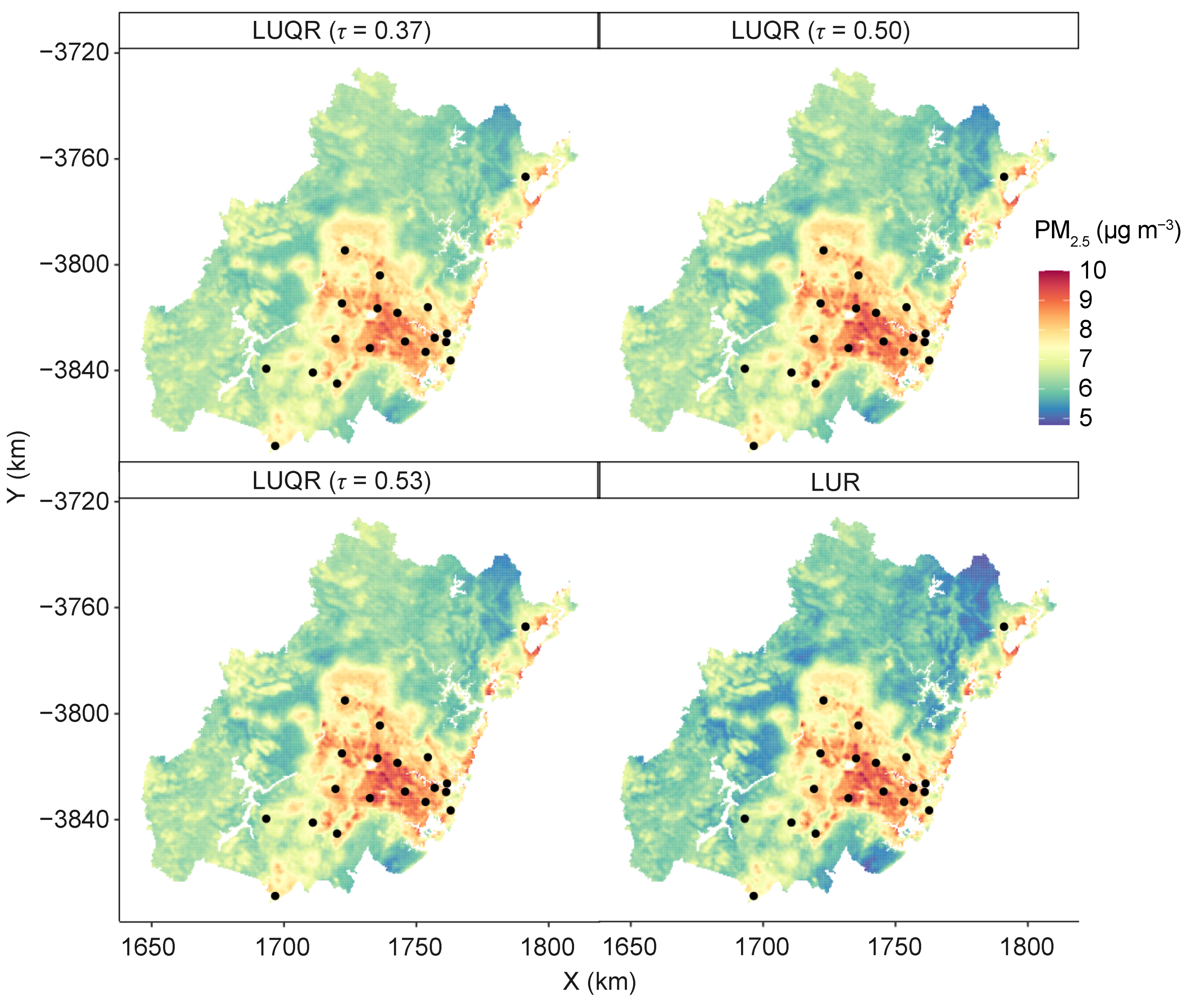
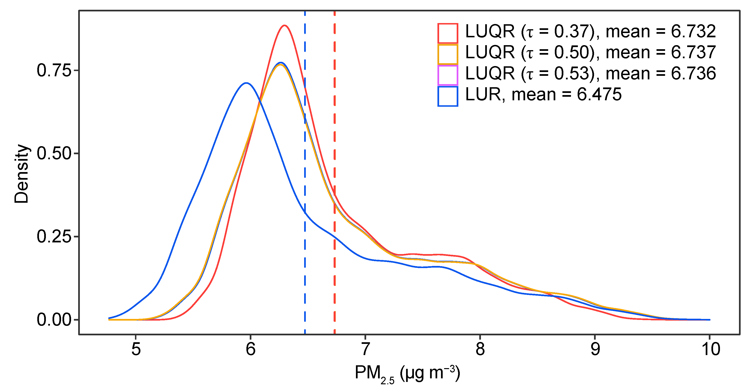
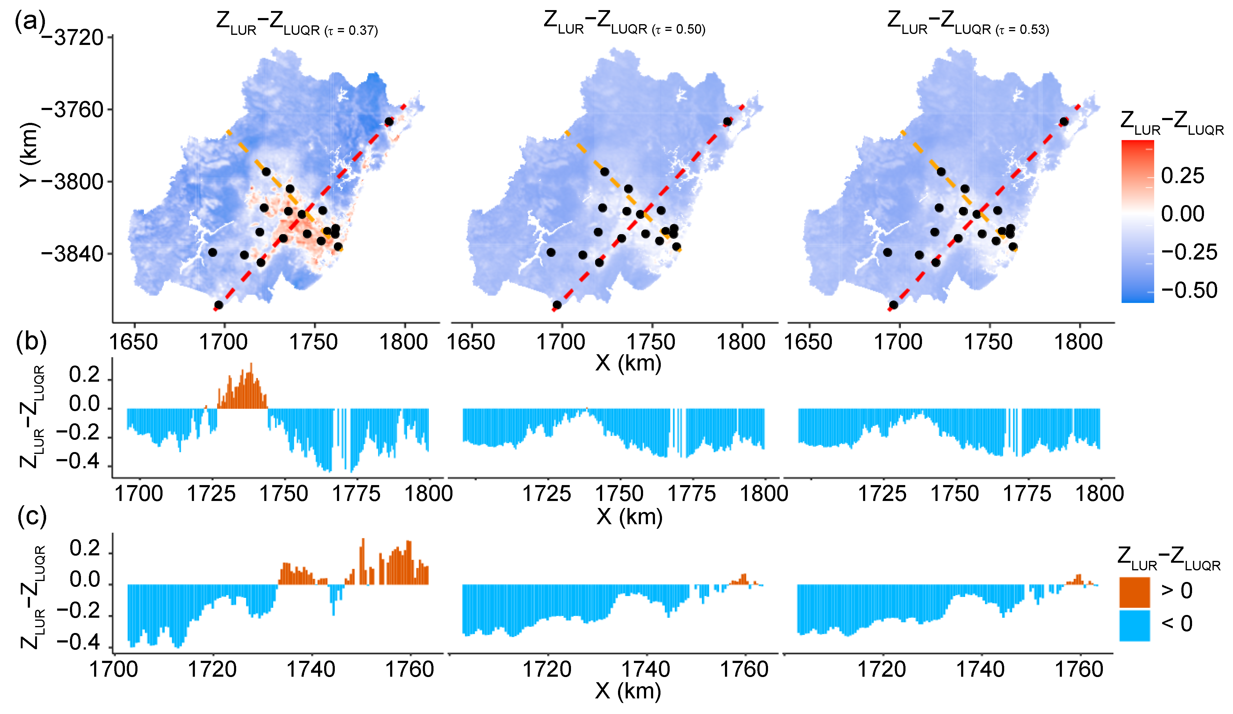
5.4. Spatial Prediction

Figure 6 shows spatial distributions of PM${}_{2.5}$ concentrations with 500 m resolution across the Greater Sydney Region using LUQR and LUR models. In general, they have similar distribution patterns of PM${}_{2.5}$ concentration, where the concentration is high in the central urban areas and near road networks, and low in outer vegetation areas. However, compared with LUQR models, the concentration tends to be overestimated in central urban areas and underestimated in outer vegetation areas by the LUR model.

Figure 7 shows the statistical density curves of grid-based predictions of PM${}_{2.5}$ concentrations derived from LUQR and LUR models. Predictions of the LUR model are generally lower than that of LUQR models. The mean value of LUR-based predictions is 6.475, and the mean values of LUQR-based predictions range from 6.732 to 6.737. The results also demonstrate that PM${}_{2.5}$ concentrations are skewed distributed across space in the study area. Compared with the LUQR models, the LUR model may overestimate the skewness of PM${}_{2.5}$ concentrations.

To more accurately present the difference between LUQR- and LUR-based predictions, Figure 8a visualizes the spatial distributions of the difference between LUQR- and LUR-based predictions. The LURQ ($\tau$ = 0.37) model and the LUR model show the highest difference in both central urban areas and outer vegetation areas among the three maps. Figure 8b,c show the difference values between LUR and LUQR models along two transects along red and orange lines shown on maps of Figure 8a. From the data of transects, we can find that in central urban areas, the concentrations predicted by the LUR model are approximately the same as or higher than the concentrations predicted by the LUQR model, but they are generally much lower than the concentrations in outer vegetation areas predicted by the LUQR model. This result is consistent with the comparison analyzed in the above model validation.

6. Discussion

6.1. Methodological Contributions

This study develops an LUQR model for the spatial prediction of PM${}_{2.5}$ concentrations with observations in a limited number of locations. The LUQR model has the following advantages in spatial predictions. First, the systematic model evaluation in this study demonstrates that the LUQR model can more accurately predict spatial distributions for small data samples than LUR models. The quantile regression model is a robust model for dealing with small data samples [18,19,20] and can more accurately predict air pollution than ordinary kriging using small data of in situ observations [24]. The integration of quantile regression in the LUQR models can effectively address the potential biased estimation in the linear model of LUR. In addition, there is no strict statistical assumptions and requirements of the sampling observation data. For instance, a linear regression model is used in the traditional LUR models, so assumptions of multivariate linear regression need to be tested and satisfied for sample data, such as normal distributions of variables and removed outliers [74,75]. On the contrary, such statistical assumptions are not required in the LUQR models because the quantile regression approach, a robust regression model, is used to fit the relationships between dependent and independent variables [76,77]. Therefore, the developed LUQR model is a reliable, accurate, and robust model for the spatial prediction of spatial issues with small data samples. It has great potential in wider fields in addition to air pollution predictions, such as the spatial predictions of soil properties, water quality attributes, and diseases.

6.2. Findings from the LUQR-Based Predictions

The LUQR-based spatial prediction maps of PM${}_{2.5}$ concentrations using a small sampling observation can present the following findings about distributions of PM${}_{2.5}$ concentrations. First, the maps show more details of air pollution than the maps predicted only using observations from the monitoring stations. The buffer-based explanatory variable selection is an essential stage to explore the impacts of multi-scale explanatory variables on air pollution. Second, more potential high-concentration areas can be identified in the maps because of using a series of explanatory variables. For instance, in this study, in addition to the central urban regions close to most of the monitoring stations, the coastal regions in the eastern part of the Greater Sydney Region also have high probabilities of high PM${}_{2.5}$ concentrations. In these regions, the PM${}_{2.5}$ monitoring stations are very sparse. Therefore, more ground monitoring works may be required in these regions to understand the PM${}_{2.5}$ concentrations and spatial characteristics. Finally, the prediction maps provide spatial and quantitative information for future optimization of the design of air pollution monitoring stations. In general, air pollution monitoring stations are set to represent regional air conditions. Thus, future monitoring stations may be added in the eastern coastal regions, and the northern and western forest, mountainous, rural, and remote areas.

6.3. Limitations and Future Recommendations

There are still limitations in this study, and more efforts are still required to deal with issues of small data samples. First, the cross-validation approach can be improved in future studies. For instance, in addition to LOOCV, a “leave-three-out” or “leave-five-out” cross-validation can be added to investigate the robustness of the LUQR and LUR models in addressing small data issues. Second, application cases with different temporal and spatial coverages can be designed and performed in future studies. In this study, we performed models for predicting annual average PM${}_{2.5}$ concentrations. Future experiment designs may include annual air pollutant predictions using data from multiple years, monthly, weekly, or daily spatial predictions; predictions for other air pollutants, such as NO${}_x$ and SO${}_2$; and spatial predictions in other study areas.

7. Conclusions

In current geographical and spatial analysis fields, it is still a challenge to accurately predict spatial distributions for mapping using samples at a small number of locations. This study developed a land use quantile regression (LUQR) model for more accurate spatial predictions of air pollution. The LUQR model is an integration of the land use regression (LUR) and the quantile regression models, which both have advantages in robust modeling with a small number of observations. The case study of the LUQR-based spatial prediction of PM${}_{2.5}$ concentrations in the Greater Sydney Region indicates that the prediction accuracy can be improved by the LUQR models compared with traditional LUR models. The model validation and result assessments demonstrate that the LUQR model is a reliable and robust model for the spatial prediction with a small sampling data set. Therefore, the developed LUQR model has great potential to be implemented in accurately predicting the distribution maps of both air pollutants at city-wide, regional, and local scales and other geospatial attributes.

References

1. Kitchin, R.; Lauriault, T.P. Small data in the era of big data. GeoJournal 2015, 80, 463–475. [Google Scholar] [CrossRef]
2. Phillips, S.J.; Dudík, M.; Elith, J.; Graham, C.H.; Lehmann, A.; Leathwick, J.; Ferrier, S. Sample selection bias and presence-only distribution models: Implications for background and pseudo-absence data. Ecol. Appl. 2009, 19, 181–197. [Google Scholar] [CrossRef] [PubMed] [Green Version]
3. Hernandez, P.A.; Graham, C.H.; Master, L.L.; Albert, D.L. The effect of sample size and species characteristics on performance of different species distribution modeling methods. Ecography 2006, 29, 773–785. [Google Scholar] [CrossRef]
4. Grinand, C.; Arrouays, D.; Laroche, B.; Martin, M.P. Extrapolating regional soil landscapes from an existing soil map: Sampling intensity, validation procedures, and integration of spatial context. Geoderma 2008, 143, 180–190. [Google Scholar] [CrossRef]
5. Oliver, M.A.; Webster, R. The Variogram and Modelling. In Basic Steps in Geostatistics: The Variogram and Kriging; Springer International Publishing: Cham, Switzerland, 2015; pp. 15–42. [Google Scholar]
6. Wang, J.; Xu, C.; Hu, M.; Li, Q.; Yan, Z.; Zhao, P.; Jones, P. A new estimate of the China temperature anomaly series and uncertainty assessment in 1900–2006. J. Geophys. Res. Atmos. 2014, 119, 1–9. [Google Scholar] [CrossRef]
7. Deng, Y.; Wang, S.; Bai, X.; Wu, L.; Cao, Y.; Li, H.; Wang, M.; Li, C.; Yang, Y.; Hu, Z.; et al. Comparison of soil moisture products from microwave remote sensing, land model, and reanalysis using global ground observations. Hydrol. Process. 2020, 34, 836–851. [Google Scholar] [CrossRef]
8. Luo, P.; Song, Y.; Huang, X.; Ma, H.; Liu, J.; Yao, Y.; Meng, L. Identifying determinants of spatio-temporal disparities in soil moisture of the Northern Hemisphere using a geographically optimal zones-based heterogeneity model. ISPRS J. Photogramm. Remote Sens. 2022, 185, 111–128. [Google Scholar] [CrossRef]
9. Liu, J.; Chai, L.; Lu, Z.; Liu, S.; Qu, Y.; Geng, D.; Song, Y.; Guan, Y.; Guo, Z.; Wang, J.; et al. Evaluation of SMAP, SMOS-IC, FY3B, JAXA, and LPRM soil moisture products over the Qinghai-Tibet plateau and its surrounding areas. Remote Sens. 2019, 11, 792. [Google Scholar] [CrossRef] [Green Version]
10. Liu, J.; Chai, L.; Dong, J.; Zheng, D.; Wigneron, J.P.; Liu, S.; Zhou, J.; Xu, T.; Yang, S.; Song, Y.; et al. Uncertainty analysis of eleven multisource soil moisture products in the third pole environment based on the three-corned hat method. Remote Sens. Environ. 2021, 255, 112225. [Google Scholar] [CrossRef]
11. Ross, Z.; Jerrett, M.; Ito, K.; Tempalski, B.; Thurston, G.D. A land use regression for predicting fine particulate matter concentrations in the New York City region. Atmos. Environ. 2007, 41, 2255–2269. [Google Scholar] [CrossRef]
12. Beelen, R.; Voogt, M.; Duyzer, J.; Zandveld, P.; Hoek, G. Comparison of the performances of land use regression modelling and dispersion modelling in estimating small-scale variations in long-term air pollution concentrations in a Dutch urban area. Atmos. Environ. 2010, 44, 4614–4621. [Google Scholar] [CrossRef]
13. Olvera, H.A.; Garcia, M.; Li, W.W.; Yang, H.; Amaya, M.A.; Myers, O.; Burchiel, S.W.; Berwick, M.; Pingitore, N.E., Jr. Principal component analysis optimization of a PM2.5 land use regression model with small monitoring network. Sci. Total Environ. 2012, 425, 27–34. [Google Scholar] [CrossRef] [PubMed] [Green Version]
14. Wang, J.; Xu, H. A novel hybrid spatiotemporal land use regression model system at the megacity scale. Atmos. Environ. 2021, 244, 117971. [Google Scholar] [CrossRef]
15. Li, Z.; Tong, X.; Ho, J.M.W.; Kwok, T.C.; Dong, G.; Ho, K.F.; Yim, S.H.L. A practical framework for predicting residential indoor PM2.5 concentration using land-use regression and machine learning methods. Chemosphere 2021, 265, 129140. [Google Scholar] [CrossRef]
16. Wong, P.Y.; Lee, H.Y.; Chen, Y.C.; Zeng, Y.T.; Chern, Y.R.; Chen, N.T.; Lung, S.C.C.; Su, H.J.; Wu, C.D. Using a land use regression model with machine learning to estimate ground level PM2.5. Environ. Pollut. 2021, 277, 116846. [Google Scholar] [CrossRef]
17. Song, Y.; Shen, Z.; Wu, P.; Viscarra Rossel, R. Wavelet geographically weighted regression for spectroscopic modelling of soil properties. Sci. Rep. 2021, 11, 17503. [Google Scholar] [CrossRef]
18. Halliru, A.M.; Loganathan, N.; Hassan, A.A.G.; Mardani, A.; Kamyab, H. Re-examining the environmental Kuznets curve hypothesis in the Economic Community of West African States: A panel quantile regression approach. J. Clean. Prod. 2020, 276, 124247. [Google Scholar] [CrossRef]
19. Tang, J.; Gao, F.; Liu, F.; Han, C.; Lee, J. Spatial heterogeneity analysis of macro-level crashes using geographically weighted Poisson quantile regression. Accid. Anal. Prev. 2020, 148, 105833. [Google Scholar] [CrossRef]
20. Xu, B.; Lin, B. Investigating drivers of CO2 emission in China’s heavy industry: A quantile regression analysis. Energy 2020, 206, 118159. [Google Scholar] [CrossRef]
21. Cade, B.S.; Noon, B.R. A gentle introduction to quantile regression for ecologists. Front. Ecol. Environ. 2003, 1, 412–420. [Google Scholar] [CrossRef]
22. Koenker, R. Quantile Regression: Economic Society Monograph Series; Cambridge University Press: Cambridge, UK, 2005. [Google Scholar]
23. Song, Y.Z.; Yang, H.L.; Peng, J.H.; Song, Y.R.; Sun, Q.; Li, Y. Estimating PM2.5 concentrations in Xi’an City using a generalized additive model with multi-source monitoring data. PLoS ONE 2015, 10, e0142149. [Google Scholar] [CrossRef] [PubMed] [Green Version]
24. Zou, B.; Luo, Y.; Wan, N.; Zheng, Z.; Sternberg, T.; Liao, Y. Performance comparison of LUR and OK in PM2.5 concentration mapping: A multidimensional perspective. Sci. Rep. 2015, 5, 8698. [Google Scholar] [CrossRef] [PubMed] [Green Version]
25. Han, L.; Zhao, J.; Gao, Y.; Gu, Z.; Xin, K.; Zhang, J. Spatial distribution characteristics of PM2.5 and PM10 in Xi’an City predicted by land use regression models. Sustain. Cities Soc. 2020, 61, 102329. [Google Scholar] [CrossRef] [PubMed]
26. Shi, Y.; Bilal, M.; Ho, H.C.; Omar, A. Urbanization and regional air pollution across South Asian developing countries–A nationwide land use regression for ambient PM2.5 assessment in Pakistan. Environ. Pollut. 2020, 266, 115145. [Google Scholar] [CrossRef]
27. Harper, A.; Baker, P.N.; Xia, Y.; Kuang, T.; Zhang, H.; Chen, Y.; Han, T.L.; Gulliver, J. Development of spatiotemporal land use regression models for PM2.5 and NO2 in Chongqing, China, and exposure assessment for the CLIMB study. Atmos. Pollut. Res. 2021, 12, 101096. [Google Scholar] [CrossRef]
28. Hoek, G.; Beelen, R.; De Hoogh, K.; Vienneau, D.; Gulliver, J.; Fischer, P.; Briggs, D. A review of land-use regression models to assess spatial variation of outdoor air pollution. Atmos. Environ. 2008, 42, 7561–7578. [Google Scholar] [CrossRef]
29. Shi, Y.; Ren, C.; Cai, M.; Lau, K.K.L.; Lee, T.C.; Wong, W.K. Assessing spatial variability of extreme hot weather conditions in Hong Kong: A land use regression approach. Environ. Res. 2019, 171, 403–415. [Google Scholar] [CrossRef]
30. Tsin, P.K.; Knudby, A.; Krayenhoff, E.S.; Brauer, M.; Henderson, S.B. Land use regression modeling of microscale urban air temperatures in greater Vancouver, Canada. Urban Clim. 2020, 32, 100636. [Google Scholar] [CrossRef]
31. Shi, Y.; Katzschner, L.; Ng, E. Modelling the fine-scale spatiotemporal pattern of urban heat island effect using land use regression approach in a megacity. Sci. Total Environ. 2018, 618, 891–904. [Google Scholar] [CrossRef]
32. Guo, Y.; Su, J.G.; Dong, Y.; Wolch, J. Application of land use regression techniques for urban greening: An analysis of Tianjin, China. Urban For. Urban Green. 2019, 38, 11–21. [Google Scholar] [CrossRef] [Green Version]
33. Chen, D.; Chen, H.; Zhao, J.; Xu, Z.; Li, W.; Xu, M. Improving spatial prediction of health risk assessment for Hg, As, Cu, and Pb in soil based on land-use regression. Environ. Geochem. Health 2020, 42, 1415–1428. [Google Scholar] [CrossRef]
34. Henderson, S.B.; Beckerman, B.; Jerrett, M.; Brauer, M. Application of land use regression to estimate long-term concentrations of traffic-related nitrogen oxides and fine particulate matter. Environ. Sci. Technol. 2007, 41, 2422–2428. [Google Scholar] [CrossRef]
35. Jones, R.R.; Hoek, G.; Fisher, J.A.; Hasheminassab, S.; Wang, D.; Ward, M.H.; Sioutas, C.; Vermeulen, R.; Silverman, D.T. Land use regression models for ultrafine particles, fine particles, and black carbon in Southern California. Sci. Total Environ. 2020, 699, 134234. [Google Scholar] [CrossRef]
36. Tularam, H.; Ramsay, L.F.; Muttoo, S.; Brunekreef, B.; Meliefste, K.; de Hoogh, K.; Naidoo, R.N. A hybrid air pollution/land use regression model for predicting air pollution concentrations in Durban, South Africa. Environ. Pollut. 2021, 274, 116513. [Google Scholar] [CrossRef]
37. Eeftens, M.; Beelen, R.; De Hoogh, K.; Bellander, T.; Cesaroni, G.; Cirach, M.; Declercq, C.; Dedele, A.; Dons, E.; De Nazelle, A.; et al. Development of land use regression models for PM2.5, PM2.5 absorbance, PM10 and PMcoarse in 20 European study areas; results of the ESCAPE project. Environ. Sci. Technol. 2012, 46, 11195–11205. [Google Scholar] [CrossRef]
38. Lee, H.J.; Chatfield, R.B.; Strawa, A.W. Enhancing the applicability of satellite remote sensing for PM2.5 estimation using MODIS deep blue AOD and land use regression in California, United States. Environ. Sci. Technol. 2016, 50, 6546–6555. [Google Scholar] [CrossRef]
39. Derdouri, A.; Murayama, Y. A comparative study of land price estimation and mapping using regression kriging and machine learning algorithms across Fukushima prefecture, Japan. J. Geogr. Sci. 2020, 30, 794–822. [Google Scholar] [CrossRef]
40. Munyati, C.; Sinthumule, N. Comparative suitability of ordinary kriging and Inverse Distance Weighted interpolation for indicating intactness gradients on threatened savannah woodland and forest stands. Environ. Sustain. Indic. 2021, 12, 100151. [Google Scholar] [CrossRef]
41. Wang, J.; Cohan, D.S.; Xu, H. Spatiotemporal ozone pollution LUR models: Suitable statistical algorithms and time scales for a megacity scale. Atmos. Environ. 2020, 237, 117671. [Google Scholar] [CrossRef]
42. Rahman, M.M.; Karunasinghe, J.; Clifford, S.; Knibbs, L.D.; Morawska, L. New insights into the spatial distribution of particle number concentrations by applying non-parametric land use regression modelling. Sci. Total Environ. 2020, 702, 134708. [Google Scholar] [CrossRef]
43. Fritsch, M.; Behm, S. Agglomeration and infrastructure effects in land use regression models for air pollution—Specification, estimation, and interpretations. Atmos. Environ. 2021, 253, 118337. [Google Scholar] [CrossRef]
44. Australian Bureau of Statistics. National, State and Territory Population; Australian Bureau of Statistics: Canberra, Australia, 2020.
45. Department of Planning, Industry and Environment, New South Wales. New South Wales Air Quality Data Services; Department of Planning, Industry and Environment: New South Wales, Parramatta, Australia, 2021. [Google Scholar]
46. Tucker, W.G. An overview of PM2.5 sources and control strategies. Fuel Process. Technol. 2000, 65, 379–392. [Google Scholar] [CrossRef]
47. Chen, R.; Yin, P.; Meng, X.; Wang, L.; Liu, C.; Niu, Y.; Liu, Y.; Liu, J.; Qi, J.; You, J.; et al. Associations between coarse particulate matter air pollution and cause-specific mortality: A nationwide analysis in 272 Chinese cities. Environ. Health Perspect. 2019, 127, 017008. [Google Scholar] [CrossRef] [Green Version]
48. Giugliano, M.; Lonati, G.; Butelli, P.; Romele, L.; Tardivo, R.; Grosso, M. Fine particulate (PM2.5–PM1) at urban sites with different traffic exposure. Atmos. Environ. 2005, 39, 2421–2431. [Google Scholar] [CrossRef]
49. Kinney, P.L.; Gichuru, M.G.; Volavka-Close, N.; Ngo, N.; Ndiba, P.K.; Law, A.; Gachanja, A.; Gaita, S.M.; Chillrud, S.N.; Sclar, E. Traffic impacts on PM2.5 air quality in Nairobi, Kenya. Environ. Sci. Policy 2011, 14, 369–378. [Google Scholar] [CrossRef] [Green Version]
50. Hu, H.; Chen, Q.; Qian, Q.; Lin, C.; Chen, Y.; Tian, W. Impacts of traffic and street characteristics on the exposure of cycling commuters to PM2.5 and PM10 in urban street environments. Build. Environ. 2021, 188, 107476. [Google Scholar] [CrossRef]
51. Xue, W.; Zhang, J.; Zhong, C.; Li, X.; Wei, J. Spatiotemporal PM2.5 variations and its response to the industrial structure from 2000 to 2018 in the Beijing-Tianjin-Hebei region. J. Clean. Prod. 2021, 279, 123742. [Google Scholar] [CrossRef]
52. Fang, D.; Yu, B. Driving mechanism and decoupling effect of PM2.5 emissions: Empirical evidence from China’s industrial sector. Energy Policy 2021, 149, 112017. [Google Scholar] [CrossRef]
53. Aguilera, R.; Corringham, T.; Gershunov, A.; Benmarhnia, T. Wildfire smoke impacts respiratory health more than fine particles from other sources: Observational evidence from Southern California. Nat. Commun. 2021, 12, 1493. [Google Scholar] [CrossRef]
54. Hua, J.; Zhang, Y.; de Foy, B.; Mei, X.; Shang, J.; Feng, C. Competing PM2.5 and NO2 holiday effects in the Beijing area vary locally due to differences in residential coal burning and traffic patterns. Sci. Total Environ. 2021, 750, 141575. [Google Scholar] [CrossRef]
55. Zhang, Y.; Shen, Z.; Sun, J.; Zhang, L.; Zhang, B.; Zou, H.; Zhang, T.; Ho, S.S.H.; Chang, X.; Xu, H.; et al. Parent, alkylated, oxygenated and nitrated polycyclic aromatic hydrocarbons in PM2.5 emitted from residential biomass burning and coal combustion: A novel database of 14 heating scenarios. Environ. Pollut. 2021, 268, 115881. [Google Scholar] [CrossRef] [PubMed]
56. Ikemori, F.; Uranishi, K.; Asakawa, D.; Nakatsubo, R.; Makino, M.; Kido, M.; Mitamura, N.; Asano, K.; Nonaka, S.; Nishimura, R.; et al. Source apportionment in PM2.5 in central Japan using positive matrix factorization focusing on small-scale local biomass burning. Atmos. Pollut. Res. 2021, 12, 162–172. [Google Scholar] [CrossRef]
57. Xu, W.; Jin, X.; Liu, M.; Ma, Z.; Wang, Q.; Zhou, Y. Analysis of spatiotemporal variation of PM2.5 and its relationship to land use in China. Atmos. Pollut. Res. 2021, 12, 101151. [Google Scholar] [CrossRef]
58. Song, J.; Zhou, S.; Peng, Y.; Xu, J.; Lin, R. Relationship between neighborhood land use structure and the spatiotemporal pattern of PM2.5 at the microscale: Evidence from the central area of Guangzhou, China. Environ. Plan. B Urban Anal. City Sci. 2021, 49, 485–500. [Google Scholar] [CrossRef]
59. Lu, D.; Mao, W.; Xiao, W.; Zhang, L. Non-Linear Response of PM2.5 Pollution to Land Use Change in China. Remote Sens. 2021, 13, 1612. [Google Scholar] [CrossRef]
60. Mhawish, A.; Banerjee, T.; Sorek-Hamer, M.; Bilal, M.; Lyapustin, A.I.; Chatfield, R.; Broday, D.M. Estimation of high-resolution PM2.5 over the indo-gangetic plain by fusion of satellite data, meteorology, and land use variables. Environ. Sci. Technol. 2020, 54, 7891–7900. [Google Scholar] [CrossRef] [PubMed]
61. Australian Bureau of Agricultural and Resource Economics and Sciences. ABARES 2021, Catchment Scale Land Use of Australia—Update December 2020; Australian Bureau of Agricultural and Resource Economics and Sciences: Canberra, Australia, 2021. [CrossRef]
62. Australian Bureau of Statistics. 1270.0.55.001—Australian Statistical Geography Standard (ASGS): Volume 1—Main Structure and Greater Capital City Statistical Areas, July 2016; Australian Bureau of Statistics: Canberra, Australia, 2017.
63. Australia, G. Digital Elevation Model (DEM) of Australia Derived from LiDAR 5 Metre Grid; Commonwealth of Australia and Geoscience Australia: Canberra, Australia, 2015. [Google Scholar]
64. Gorelick, N.; Hancher, M.; Dixon, M.; Ilyushchenko, S.; Thau, D.; Moore, R. Google Earth Engine: Planetary-scale geospatial analysis for everyone. Remote Sens. Environ. 2017, 202, 18–27. [Google Scholar] [CrossRef]
65. Sheng, Q.; Zhang, Y.; Zhu, Z.; Li, W.; Xu, J.; Tang, R. An experimental study to quantify road greenbelts and their association with PM2.5 concentration along city main roads in Nanjing, China. Sci. Total Environ. 2019, 667, 710–717. [Google Scholar] [CrossRef]
66. Witkowska, A.; Lewandowska, A.U.; Saniewska, D.; Falkowska, L.M. Effect of agriculture and vegetation on carbonaceous aerosol concentrations (PM2.5 and PM10) in Puszcza Borecka National Nature Reserve (Poland). Air Qual. Atmos. Health 2016, 9, 761–773. [Google Scholar] [CrossRef] [Green Version]
67. Song, Z.; Li, R.; Qiu, R.; Liu, S.; Tan, C.; Li, Q.; Ge, W.; Han, X.; Tang, X.; Shi, W.; et al. Global land surface temperature influenced by vegetation cover and PM2.5 from 2001 to 2016. Remote Sens. 2018, 10, 2034. [Google Scholar] [CrossRef] [Green Version]
68. Didan, K. MOD13A1 MODIS/Terra Vegetation Indices 16-Day L3 Global 500m SIN Grid V006, NASA EOSDIS Land Processes DAAC. 2015. Available online: https://lpdaac.usgs.gov/products/mod13a1v006/ (accessed on 30 October 2021).
69. Hair, J.; Anderson, R.; Babin, B.; Black, W. Multivariate Data Analysis: A Global Perspective (Vol. 7); Pearson Upper Saddle River: Hoboken, NJ, USA, 2010. [Google Scholar]
70. Song, Y.; Ge, Y.; Wang, J.; Ren, Z.; Liao, Y.; Peng, J. Spatial distribution estimation of malaria in northern China and its scenarios in 2020, 2030, 2040 and 2050. Malar. J. 2016, 15, 345. [Google Scholar] [CrossRef] [Green Version]
71. Ge, Y.; Song, Y.; Wang, J.; Liu, W.; Ren, Z.; Peng, J.; Lu, B. Geographically weighted regression-based determinants of malaria incidences in northern China. Trans. GIS 2017, 21, 934–953. [Google Scholar] [CrossRef]
72. Buchinsky, M. Estimating the asymptotic covariance matrix for quantile regression models a Monte Carlo study. J. Econom. 1995, 68, 303–338. [Google Scholar] [CrossRef]
73. Koenker, R.; Machado, J.A. Goodness of fit and related inference processes for quantile regression. J. Am. Stat. Assoc. 1999, 94, 1296–1310. [Google Scholar] [CrossRef]
74. Bernales, A.; Antolihao, J.; Samonte, C.; Campomanes, F.; Rojas, R.; Silapan, J. Modelling the relationship between land surface temperature and landscape patterns of land use land cover classification using multi linear regression models. Int. Arch. Photogramm. Remote Sens. Spat. Inf. Sci. 2016, 41, 851–856. [Google Scholar] [CrossRef] [Green Version]
75. Ross, Z.; English, P.B.; Scalf, R.; Gunier, R.; Smorodinsky, S.; Wall, S.; Jerrett, M. Nitrogen dioxide prediction in Southern California using land use regression modeling: Potential for environmental health analyses. J. Expo. Sci. Environ. Epidemiol. 2006, 16, 106–114. [Google Scholar] [CrossRef]
76. John, O.O. Robustness of quantile regression to outliers. Am. J. Appl. Math. Stat. 2015, 3, 86–88. [Google Scholar]
77. Furno, M.; Vistocco, D. Quantile Regression: Estimation and Simulation; John Wiley & Sons: Hoboken, NJ, USA, 2018; Volume 216. [Google Scholar]
Figure 1. Spatial distributions of air quality monitoring stations and annual mean PM 2.5 in Great Sydney Region, New South Wales, Australia.
Remotesensing 14 01370 g001
Figure 2. Spatial distributions of explanatory variables: land use (a), population density (b), road network (c), elevation (d), and vegetation (NDVI) (e).
Remotesensing 14 01370 g002
Figure 3. Coefficients of explanatory variables in the land use quantile regression (LUQR) model for PM 2.5 prediction. The orange lines are coefficients by quantiles in LUQR model, and orange areas show the 95% CIs of LUQR coefficients. The blue horizontal lines are coefficients of the linear regression model, and the blue dashed lines are the 95% confidence intervals (CIs) of the coefficients in the linear regression model.
Remotesensing 14 01370 g003
Figure 4. The leave-one-out cross-validation (LOOCV) of land use quantile regression (LUQR) models of PM 2.5 with different values of quantile parameter τ . (a) Comparison of R 2 of LUR (dashed orange line) and LUQR (orange line); (b) Comparison of RMSE (blue) and MAE (green) of LUR (dash lines) and LUQR (lines).
Remotesensing 14 01370 g004
Figure 5. Comparison of LOOCV results between LUR and LUQR models: relationship between observations and predictions of PM 2.5 concentrations in LOOCV (a) and relationship between predictions and residuals of PM 2.5 concentrations in LOOCV (b).
Remotesensing 14 01370 g005
Figure 6. Spatial predictions of PM 2.5 concentrations using LUQR ( τ = 0.37), LUQR ( τ = 0.50), LUQR ( τ = 0.53) and LUR models.
Remotesensing 14 01370 g006
Figure 7. Density distributions of PM 2.5 concentrations predicted using LUQR and LUR models.
Remotesensing 14 01370 g007
Figure 8. Spatial distributions of the difference between LUR-based prediction ( Z L U R ) and LUQR-based prediction ( Z L U Q R ) (a), and transect along red (b) and orange (c) lines. (“Z” is predictions of models).
Remotesensing 14 01370 g008