
Estimating Forest Soil Properties for Humus Assessment—Is Vis-NIR the Way to Go?

 , ,
, ,
Abstract
:1. Introduction
2. Methods
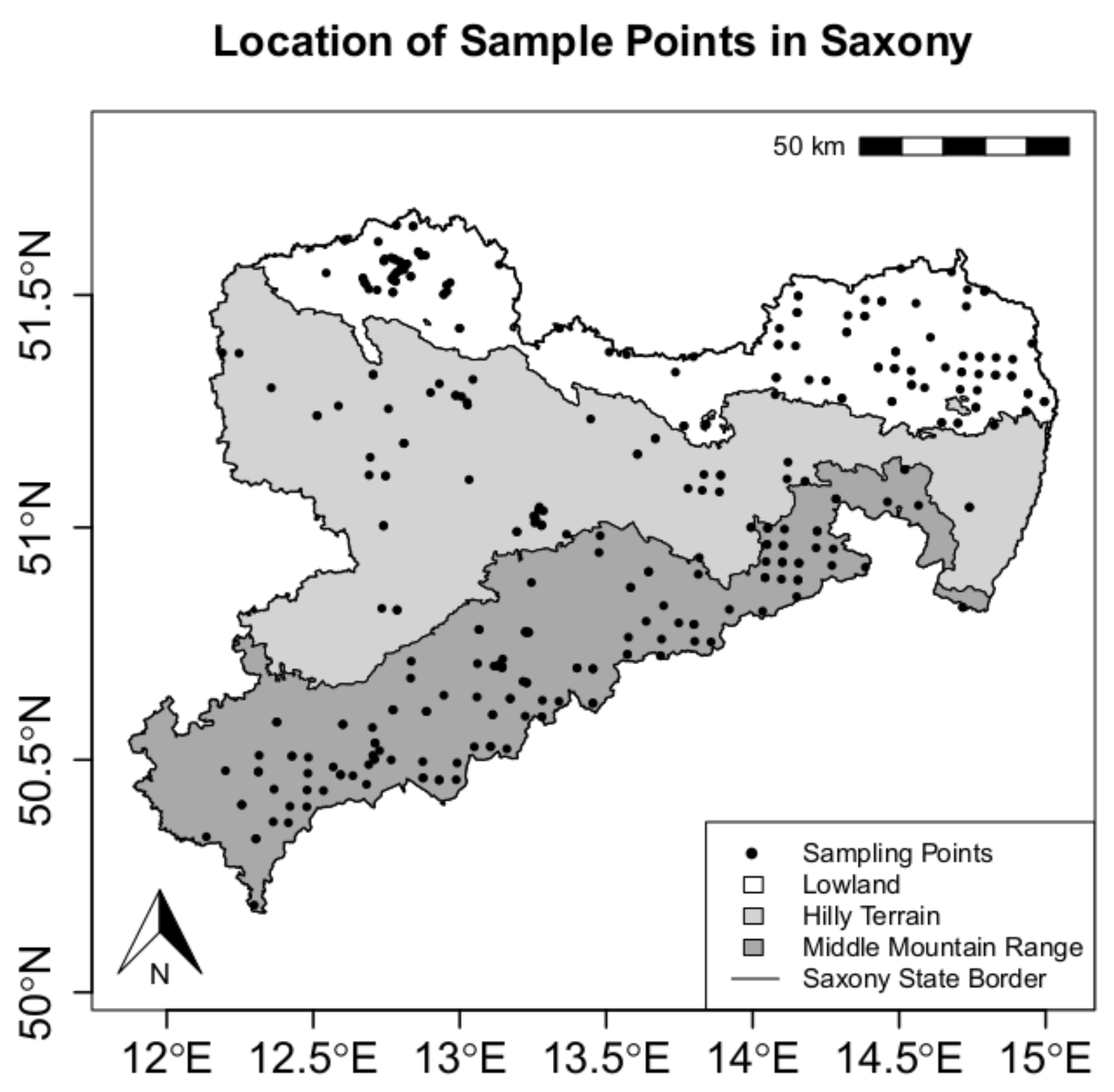
2.1. Study Area
2.2. Vis-NIR Spectroscopy
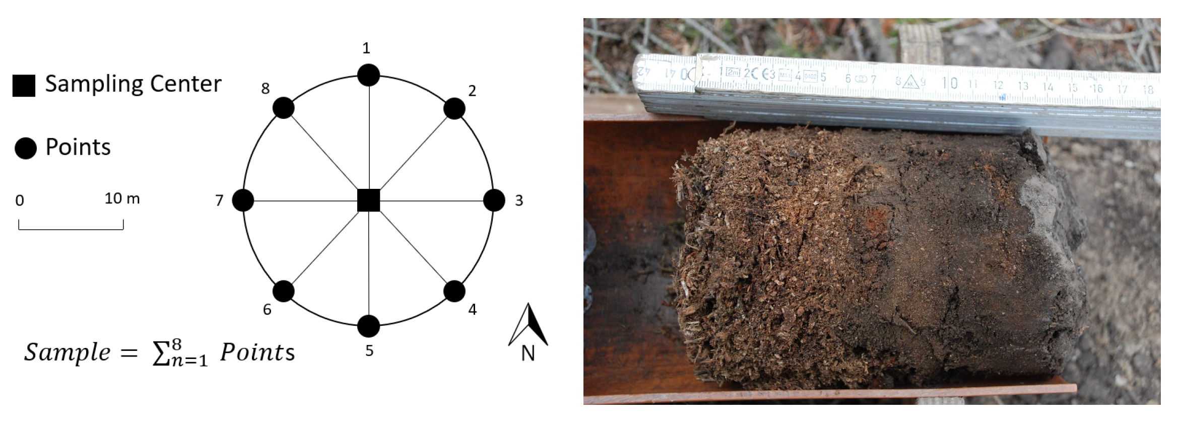
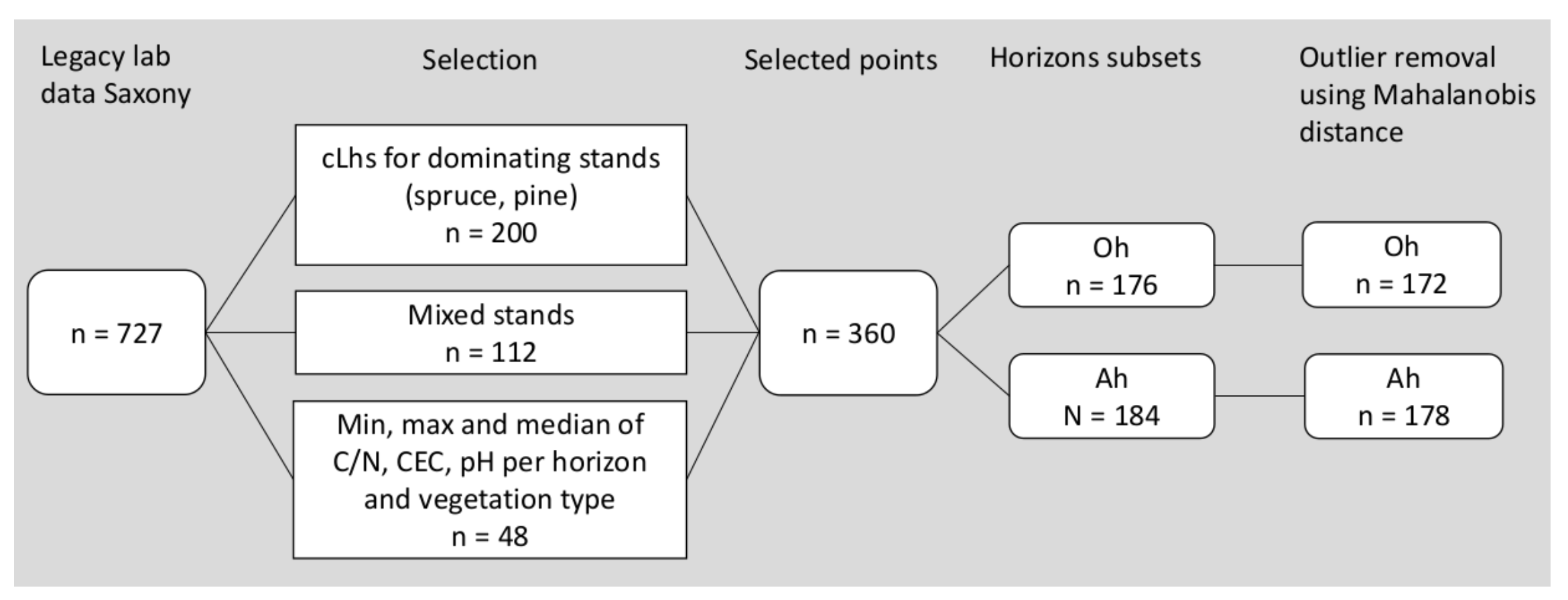
2.3. Soil Samples and Laboratory Analysis
2.4. Spectral Measurements and Pre-Processing
2.5. Regression Approaches
2.6. Spectral Model Tuning and Validation
2.7. Evaluate Feasibility for Soil Mapping
3. Results
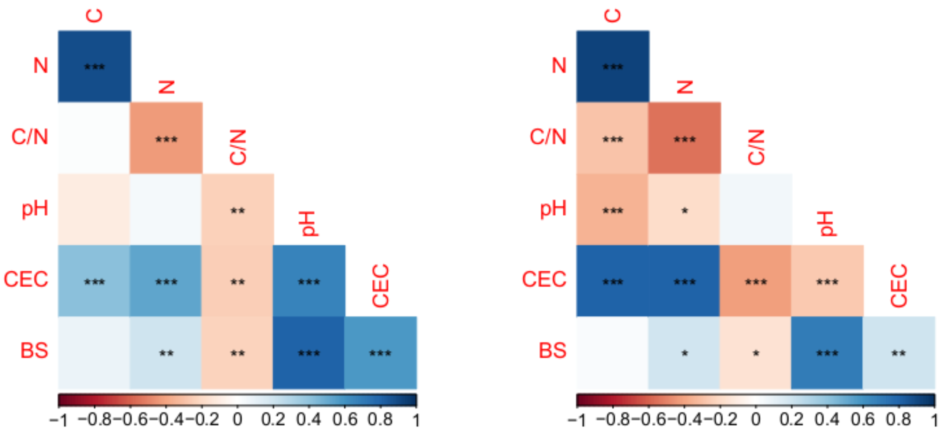
3.1. Descriptive Statistics of Soil Properties
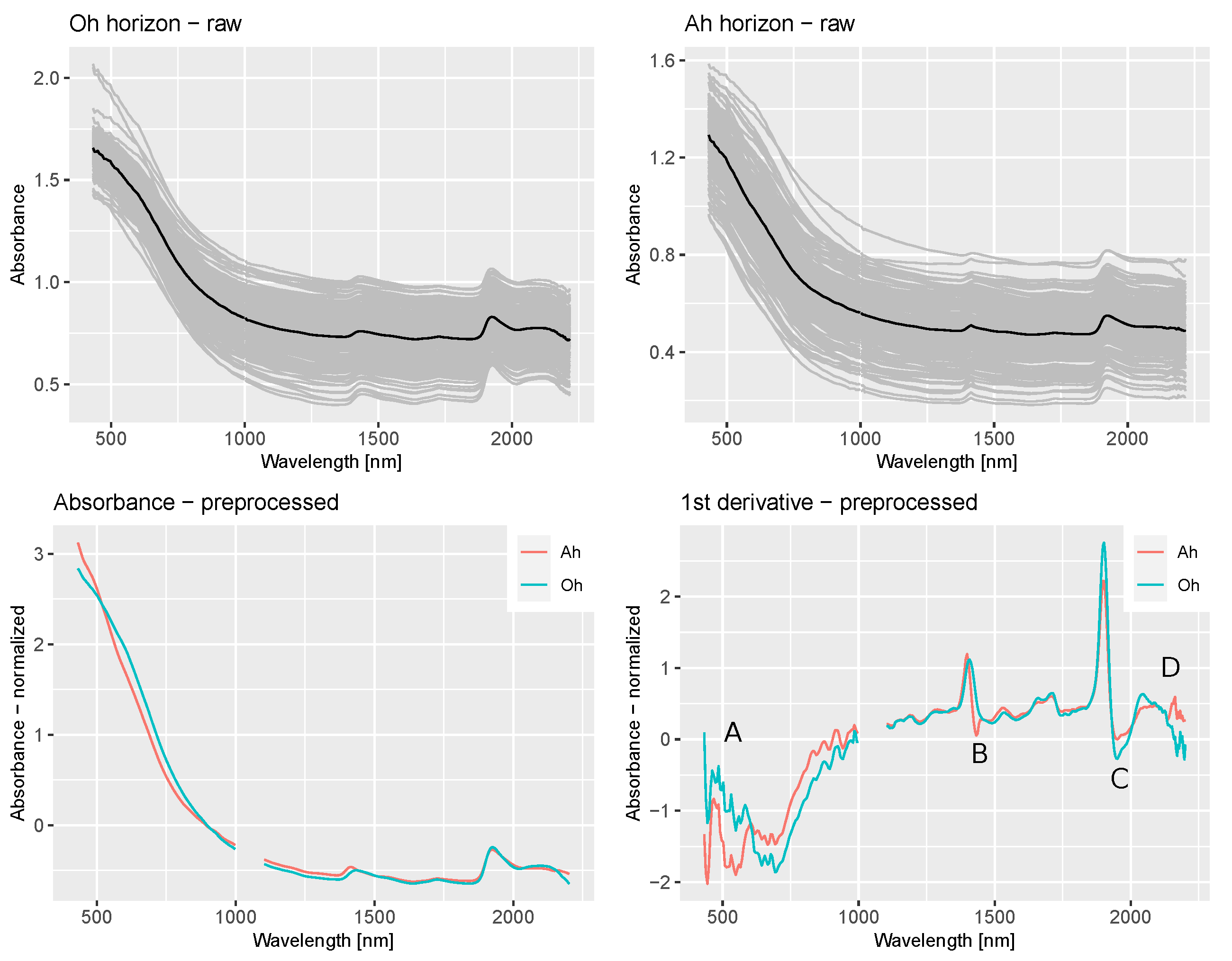
3.2. Spectral Differences between Horizons
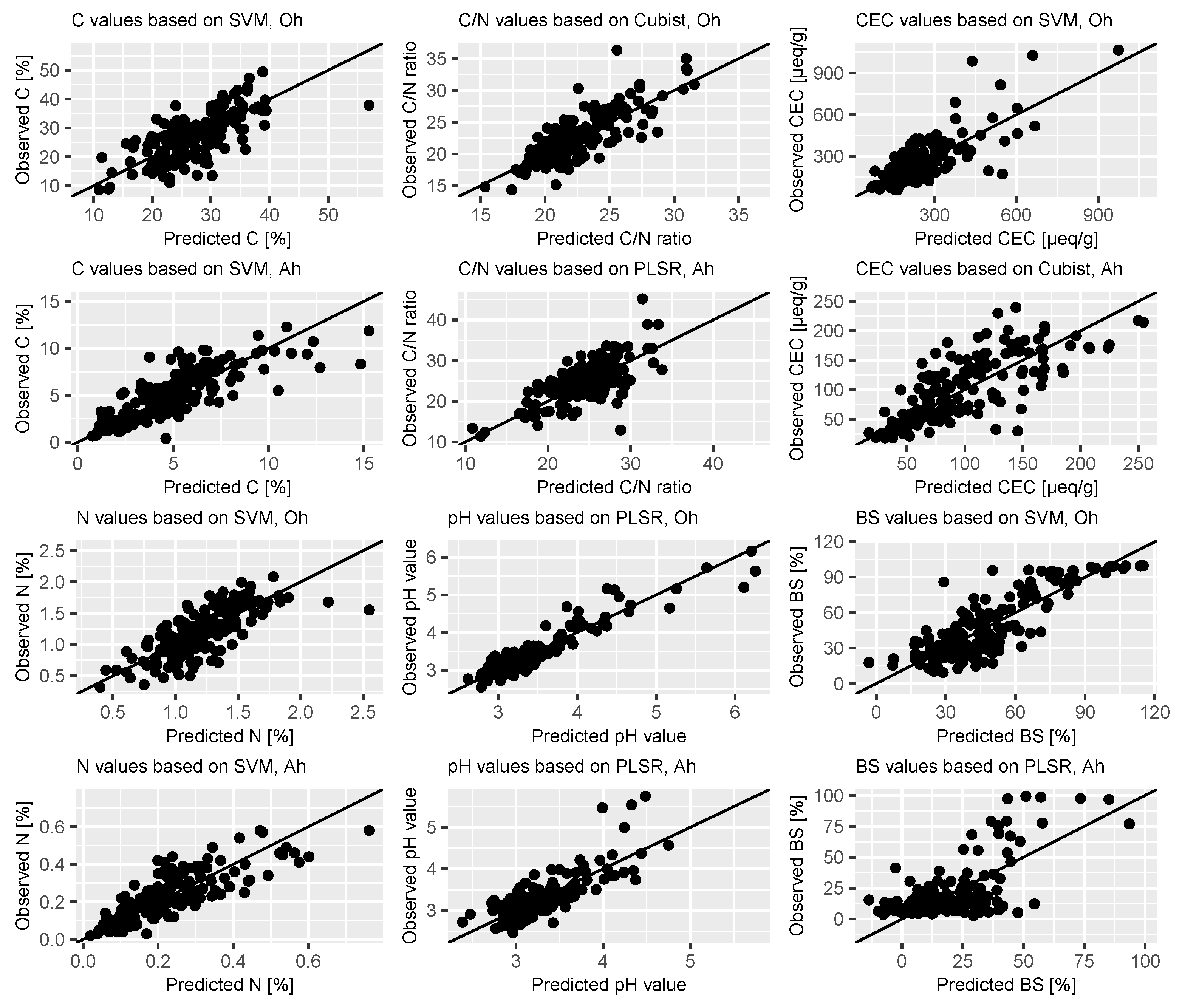
3.3. Predicting Oh Properties
3.4. Predicting Ah Properties
3.5. Classification for Mapping Purposes
4. Discussion
4.1. Data Ranges of Soil Properties
4.2. Spectral Behaviour
4.3. Predicting Oh Properties
4.4. Predicting Ah Properties
4.5. Classification Based on pH Values
4.6. Further Implications
5. Conclusions
Author Contributions
Funding
Data Availability Statement
Acknowledgments
Conflicts of Interest
Abbreviations
| vis | visual |
| NIR | near infrared |
| C | carbon |
| N | nitrogen |
| CEC | cation exchange capacity |
| BS | base saturation |
| NFSI | national forest soil inventory |
| PSS | proximal soil sensing |
| vis-NIRS | visual and near-infrared reflectance spectroscopy |
| SOC | soil organic carbon |
| PLSR | partial least squares regression |
| SVM | support vector machine |
| RMSE | root mean square error |
| RPIQ | ratio of performance to interquartile |
| RPD | ratio of performance to deviation |
References
- Schuldt, B.; Buras, A.; Arend, M.; Vitasse, Y.; Beierkuhnlein, C.; Damm, A.; Gharun, M.; Grams, T.E.; Hauck, M.; Hajek, P.; et al. A first assessment of the impact of the extreme 2018 summer drought on Central European forests. Basic Appl. Ecol. 2020, 45, 86–103. [Google Scholar] [CrossRef]
- Allen, C.D.; Macalady, A.K.; Chenchouni, H.; Bachelet, D.; McDowell, N.; Vennetier, M.; Kitzberger, T.; Rigling, A.; Breshears, D.D.; Hogg, E.T.; et al. A global overview of drought and heat-induced tree mortality reveals emerging climate change risks for forests. For. Ecol. Manag. 2010, 259, 660–684. [Google Scholar] [CrossRef] [Green Version]
- Nussbaum, M.; Spiess, K.; Baltensweiler, A.; Grob, U.; Keller, A.; Greiner, L.; Schaepman, M.E.; Papritz, A.J. Evaluation of digital soil mapping approaches with large sets of environmental covariates. Soil 2018, 4, 1–22. [Google Scholar] [CrossRef] [Green Version]
- Conen, F.; Zerva, A.; Arrouays, D.; Jolivet, C.; Jarvis, P.G.; Grace, J.; Mencuccini, M. The carbon balance of forest soils: Detectability of changes in soil carbon stocks in temperate and boreal forests. Carbon Balance For. Biomes 2004, 9, 233–247. [Google Scholar]
- Petzold, R.; Benning, R.; Gauer, J. Bodeninformationen in den verschiedenen Standortserkundungssystemen Deutschlands: Gegenwärtiger Stand und Perspektiven. Wald. Landsch. Nat. 2016, 16, 7–17. [Google Scholar]
- Prescott, C.E.; Maynard, D.G.; Laiho, R. Humus in northern forests: Friend or foe? For. Ecol. Manag. 2000, 133, 23–36. [Google Scholar] [CrossRef]
- Binkley, D.; Fisher, R.F. Ecology and Management of Forest Soils, 5th ed.; Wiley: Hoboken, NJ, USA, 2020. [Google Scholar]
- Schulze, G.; Kopp, D. Anleitung für die forstliche Standortserkundung im nordostdeutschen Tiefland. Standortserkundungsanleitung 2013, 95, 1–178. [Google Scholar]
- Wellbrock, N.; Ahrends, B.; Bögelein, R.; Bolte, A.; Eickenscheidt, N.; Grüneberg, E.; König, N.; Schmitz, A.; Fleck, S.; Ziche, D. Concept and methodology of the national forest soil inventory. In Status and Dynamics of Forests in Germany; Springer: Cham, Switzerland, 2019; pp. 1–28. [Google Scholar]
- Rossel, R.V.; Adamchuk, V.; Sudduth, K.; McKenzie, N.; Lobsey, C. Proximal soil sensing: An effective approach for soil measurements in space and time. In Advances in Agronomy; Elsevier: Amsterdam, The Netherland, 2011; Volume 113, pp. 243–291. [Google Scholar]
- Viscarra Rossel, R.; Lark, R. Improved analysis and modelling of soil diffuse reflectance spectra using wavelets. Eur. J. Soil Sci. 2009, 60, 453–464. [Google Scholar] [CrossRef]
- Nocita, M.; Stevens, A.; van Wesemael, B.; Aitkenhead, M.; Bachmann, M.; Barthès, B.; Dor, E.B.; Brown, D.J.; Clairotte, M.; Csorba, A.; et al. Soil spectroscopy: An alternative to wet chemistry for soil monitoring. Adv. Agron. 2015, 132, 139–159. [Google Scholar]
- Reeves, J.; McCarty, G.; Meisinger, J. Near infrared reflectance spectroscopy for the analysis of agricultural soils. J. Near Infrared Spectrosc. 1999, 7, 179–193. [Google Scholar] [CrossRef]
- Kuang, B.; Mouazen, A. Calibration of visible and near infrared spectroscopy for soil analysis at the field scale on three European farms. Eur. J. Soil Sci. 2011, 62, 629–636. [Google Scholar] [CrossRef]
- Rossel, R.V.; Walvoort, D.; McBratney, A.; Janik, L.J.; Skjemstad, J. Visible, near infrared, mid infrared or combined diffuse reflectance spectroscopy for simultaneous assessment of various soil properties. Geoderma 2006, 131, 59–75. [Google Scholar] [CrossRef]
- Ribeiro, S.G.; Teixeira, A.d.S.; de Oliveira, M.R.R.; Costa, M.C.G.; Araújo, I.C.d.S.; Moreira, L.C.J.; Lopes, F.B. Soil Organic Carbon Content Prediction Using Soil-Reflected Spectra: A Comparison of Two Regression Methods. Remote Sens. 2021, 13, 4752. [Google Scholar] [CrossRef]
- Pietrzykowski, M.; Chodak, M. Near infrared spectroscopy—A tool for chemical properties and organic matter assessment of afforested mine soils. Ecol. Eng. 2014, 62, 115–122. [Google Scholar] [CrossRef]
- Ludwig, B.; Vormstein, S.; Niebuhr, J.; Heinze, S.; Marschner, B.; Vohland, M. Estimation accuracies of near infrared spectroscopy for general soil properties and enzyme activities for two forest sites along three transects. Geoderma 2017, 288, 37–46. [Google Scholar] [CrossRef]
- Thomas, F.; Petzold, R.; Becker, C.; Werban, U. Application of Low-Cost MEMS Spectrometers for Forest Topsoil Properties Prediction. Sensors 2021, 21, 3927. [Google Scholar] [CrossRef]
- Liu, S.; Shen, H.; Chen, S.; Zhao, X.; Biswas, A.; Jia, X.; Shi, Z.; Fang, J. Estimating forest soil organic carbon content using vis-NIR spectroscopy: Implications for large-scale soil carbon spectroscopic assessment. Geoderma 2019, 348, 37–44. [Google Scholar] [CrossRef]
- Pinheiro, É.F.; Ceddia, M.B.; Clingensmith, C.M.; Grunwald, S.; Vasques, G.M. Prediction of soil physical and chemical properties by visible and near-infrared diffuse reflectance spectroscopy in the central Amazon. Remote Sens. 2017, 9, 293. [Google Scholar] [CrossRef] [Green Version]
- Gholizadeh, A.; Viscarra Rossel, R.A.; Saberioon, M.; Borůvka, L.; Kratina, J.; Pavlů, L. National-scale spectroscopic assessment of soil organic carbon in forests of the Czech Republic. Geoderma 2021, 385, 114832. [Google Scholar] [CrossRef]
- Ertlen, D.; Schwartz, D.; Trautmann, M.; Webster, R.; Brunet, D. Discriminating between organic matter in soil from grass and forest by near-infrared spectroscopy. Eur. J. Soil Sci. 2010, 61, 207–216. [Google Scholar] [CrossRef]
- Wellbrock, N.; Grüneberg, E.; Ziche, D.; Eickenscheidt, N.; Holzhausen, M.; Höhle, J.; Gemballa, R.; Andreae, H. Entwicklung einer Methodik zur stichprobengestützten Erfassung und Regionalisierung von Zustandseigenschaften der Waldstandorte; Thünen Report 36; Johann Heinrich von Thünen-Institut: Braunschweig, Germany, 2015. [Google Scholar] [CrossRef]
- Rossel, R.V.; Behrens, T. Using data mining to model and interpret soil diffuse reflectance spectra. Geoderma 2010, 158, 46–54. [Google Scholar] [CrossRef]
- Rossel, R.V.; Behrens, T.; Ben-Dor, E.; Brown, D.; Demattê, J.; Shepherd, K.D.; Shi, Z.; Stenberg, B.; Stevens, A.; Adamchuk, V.; et al. A global spectral library to characterize the world’s soil. Earth-Sci. Rev. 2016, 155, 198–230. [Google Scholar] [CrossRef] [Green Version]
- Christy, C.D. Real-time measurement of soil attributes using on-the-go near infrared reflectance spectroscopy. Comput. Electron. Agric. 2008, 61, 10–19. [Google Scholar] [CrossRef]
- Gubler, A. Quantitative Estimations of Soil Properties by Visible and Near Infrared Spectroscopy: Applications for Laboratory and Field Measurements. Ph.D. Thesis, University of Bern, Bern, Switzerland, 2011. [Google Scholar]
- Knadel, M.; Masís-Meléndez, F.; de Jonge, L.W.; Moldrup, P.; Arthur, E.; Greve, M.H. Assessing soil water repellency of a sandy field with visible near infrared spectroscopy. J. Near Infrared Spectrosc. 2016, 24, 215–224. [Google Scholar] [CrossRef] [Green Version]
- Baumgardner, M.F.; Silva, L.F.; Biehl, L.L.; Stoner, E.R. Reflectance properties of soils. Adv. Agron. 1986, 38, 1–44. [Google Scholar]
- Hunt, G.R. Spectral signatures of particulate minerals in the visible and near infrared. Geophysics 1977, 42, 501–513. [Google Scholar] [CrossRef] [Green Version]
- Fourty, T.; Baret, F.; Jacquemoud, S.; Schmuck, G.; Verdebout, J. Leaf optical properties with explicit description of its biochemical composition: Direct and inverse problems. Remote Sens. Environ. 1996, 56, 104–117. [Google Scholar] [CrossRef]
- Ben-Dor, E.; Banin, A. Near-infrared analysis as a rapid method to simultaneously evaluate several soil properties. Soil Sci. Soc. Am. J. 1995, 59, 364–372. [Google Scholar] [CrossRef]
- Stenberg, B.; Rossel, R.A.V.; Mouazen, A.M.; Wetterlind, J. Visible and near infrared spectroscopy in soil science. In Advances in Agronomy; Elsevier: Amsterdam, The Netherlands, 2010; Volume 107, pp. 163–215. [Google Scholar]
- Xu, D.; Ma, W.; Chen, S.; Jiang, Q.; He, K.; Shi, Z. Assessment of important soil properties related to Chinese Soil Taxonomy based on vis–NIR reflectance spectroscopy. Comput. Electron. Agric. 2018, 144, 1–8. [Google Scholar] [CrossRef]
- Gutachterausschuss Forstliche Analytik. Handbuch Forstliche Analytik. Eine Loseblatt-Sammlung der Analysemethoden im Forstbereich. 2014. Available online: https://www.nw-fva.de/fileadmin/nwfva/publikationen/pdf/konig_handbuch_forstliche.pdf (accessed on 28 September 2021).
- DIN ISO 10390: 2005; Bodenbeschaffenheit—Bestimmung des pH-Wertes. Deutsches Insitut für Normung: Berlin, Germany, 2005.
- Höhle, J.; Bielefeldt, J.; Dühnelt, P.; König, N.; Ziche, D.; Eickenscheidt, N.; Grüneberg, E.; Hilbrig, L.; Wellbrock, N. Bodenzustandserhebung im Wald-Dokumentation und Harmonisierung der Methoden; Technical Report, Thünen Working Paper; Johann Heinrich von Thünen-Institut: Braunschweig, Germany, 2018. [Google Scholar]
- DIN 10694; Bestimmung des Organischen Kohlenstoffgehaltes und des Gesamtkohlenstoffgehaltes Nach Trockener Verbrennung (Elementaranalyse); Deutsche Normen (ed. Fachnormenausschuß Wasserwesen, FNW, im DIN Deutsches Institut für Normung e.V.). Beuth Verlag: Berlin, Germany, 1994.
- Avian Technologies. Fluorilon Gray Scale Standards & Targets. 2019. Available online: https://aviantechnologies.com/product/gray-scale-standards/ (accessed on 13 June 2019).
- Mac Arthur, A.; MacLellan, C.J.; Malthus, T. The fields of view and directional response functions of two field spectroradiometers. IEEE Trans. Geosci. Remote Sens. 2012, 50, 3892–3907. [Google Scholar] [CrossRef]
- Rinnan, Å.; Van Den Berg, F.; Engelsen, S.B. Review of the most common pre-processing techniques for near-infrared spectra. TrAC Trends Anal. Chem. 2009, 28, 1201–1222. [Google Scholar] [CrossRef]
- Savitzky, A.; Golay, M.J. Smoothing and differentiation of data by simplified least squares procedures. Anal. Chem. 1964, 36, 1627–1639. [Google Scholar] [CrossRef]
- Stevens, A.; Nocita, M.; Tóth, G.; Montanarella, L.; van Wesemael, B. Prediction of soil organic carbon at the European scale by visible and near infrared reflectance spectroscopy. PLoS ONE 2013, 8, e66409. [Google Scholar] [CrossRef]
- Barnes, R.; Dhanoa, M.S.; Lister, S.J. Standard normal variate transformation and de-trending of near-infrared diffuse reflectance spectra. Appl. Spectrosc. 1989, 43, 772–777. [Google Scholar] [CrossRef]
- Stevens, A.; Ramirez-Lopez, L. An Introduction to the Prospectr Package, Version 0.1.3; R Core Team: Vienna, Austria, 2013.
- Filzmoser, P.; Gschwandtner, M. Mvoutlier: Multivariate Outlier Detection Based on Robust Methods; Version 2.0.9; R Core Team: Vienna, Austria, 2018. [Google Scholar]
- Filzmoser, P.; Garrett, R.G.; Reimann, C. Multivariate outlier detection in exploration geochemistry. Comput. Geosci. 2005, 31, 579–587. [Google Scholar] [CrossRef]
- R Core Team. R: A Language and Environment for Statistical Computing; R Foundation for Statistical Computing: Vienna, Austria, 2018. [Google Scholar]
- Leone, A.; Viscarra-Rossel, R.; Amenta, P.; Buondonno, A. Prediction of soil properties with PLSR and vis-NIR spectroscopy: Application to mediterranean soils from Southern Italy. Curr. Anal. Chem. 2012, 8, 283–299. [Google Scholar] [CrossRef]
- Chang, C.W.; Laird, D.A. Near-infrared reflectance spectroscopic analysis of soil C and N. Soil Sci. 2002, 167, 110–116. [Google Scholar] [CrossRef]
- Reeves, J.B., III. Near-versus mid-infrared diffuse reflectance spectroscopy for soil analysis emphasizing carbon and laboratory versus on-site analysis: Where are we and what needs to be done? Geoderma 2010, 158, 3–14. [Google Scholar] [CrossRef]
- Shi, T.; Cui, L.; Wang, J.; Fei, T.; Chen, Y.; Wu, G. Comparison of multivariate methods for estimating soil total nitrogen with visible/near-infrared spectroscopy. Plant Soil 2013, 366, 363–375. [Google Scholar] [CrossRef]
- Sorenson, P.T.; Small, C.; Tappert, M.; Quideau, S.A.; Drozdowski, B.; Underwood, A.; Janz, A. Monitoring organic carbon, total nitrogen, and pH for reclaimed soils using field reflectance spectroscopy. Can. J. Soil Sci. 2017, 97, 241–248. [Google Scholar] [CrossRef]
- Wold, S.; Martens, H.; Wold, H. The multivariate calibration problem in chemistry solved by the PLS method. In Matrix Pencils; Springer: Cham, Switzerland, 1983; pp. 286–293. [Google Scholar]
- Ramirez-Lopez, L.; Behrens, T.; Schmidt, K.; Stevens, A.; Demattê, J.A.M.; Scholten, T. The spectrum-based learner: A new local approach for modeling soil vis–NIR spectra of complex datasets. Geoderma 2013, 195, 268–279. [Google Scholar] [CrossRef]
- Hastie, T.; Tibshirani, R.; Friedman, J. The Elements of Statistical Learning: Data Mining, Inference, and Prediction; Springer Science & Business Media: Cham, Switzerland, 2009. [Google Scholar]
- Cortes, C.; Vapnik, V. Support-vector networks. Mach. Learn. 1995, 20, 273–297. [Google Scholar] [CrossRef]
- Müller, A.C.; Guido, S. Introduction to Machine Learning with Python: A Guide For Data Scientists, 1st ed.; O’Reilly Media, Inc.: Newton, MA, USA, 2016. [Google Scholar]
- Quinlan, J.R. Learning with continuous classes. In Proceedings of the 5th Australian Joint Conference on Artificial Intelligence, World Scientific, Canberra, ACT, Australia, 2–5 December 1992; Volume 92, pp. 343–348. [Google Scholar]
- Appelhans, T.; Mwangomo, E.; Hardy, D.R.; Hemp, A.; Nauss, T. Evaluating machine learning approaches for the interpolation of monthly air temperature at Mt. Kilimanjaro, Tanzania. Spat. Stat. 2015, 14, 91–113. [Google Scholar] [CrossRef] [Green Version]
- Morellos, A.; Pantazi, X.E.; Moshou, D.; Alexandridis, T.; Whetton, R.; Tziotzios, G.; Wiebensohn, J.; Bill, R.; Mouazen, A.M. Machine learning based prediction of soil total nitrogen, organic carbon and moisture content by using VIS-NIR spectroscopy. Biosyst. Eng. 2016, 152, 104–116. [Google Scholar] [CrossRef] [Green Version]
- Walton, J.T. Subpixel urban land cover estimation. Photogramm. Eng. Remote Sens. 2008, 74, 1213–1222. [Google Scholar] [CrossRef] [Green Version]
- Kuhn, M. caret: Classification and Regression Training; Version 6.0-81; R Core Team: Vienna, Austria, 2018. [Google Scholar]
- Nash, J.E.; Sutcliffe, J.V. River flow forecasting through conceptual models part I—A discussion of principles. J. Hydrol. 1970, 10, 282–290. [Google Scholar] [CrossRef]
- Bellon-Maurel, V.; Fernandez-Ahumada, E.; Palagos, B.; Roger, J.M.; McBratney, A. Critical review of chemometric indicators commonly used for assessing the quality of the prediction of soil attributes by NIR spectroscopy. TrAC Trends Anal. Chem. 2010, 29, 1073–1081. [Google Scholar] [CrossRef]
- Chang, C.W.; Laird, D.A.; Mausbach, M.J.; Hurburgh, C.R. Near-infrared reflectance spectroscopy–principal components regression analyses of soil properties. Soil Sci. Soc. Am. J. 2001, 65, 480–490. [Google Scholar] [CrossRef] [Green Version]
- Nocita, M.; Stevens, A.; Toth, G.; Panagos, P.; van Wesemael, B.; Montanarella, L. Prediction of soil organic carbon content by diffuse reflectance spectroscopy using a local partial least square regression approach. Soil Biol. Biochem. 2014, 68, 337–347. [Google Scholar] [CrossRef]
- Vohland, M.; Ludwig, M.; Thiele-Bruhn, S.; Ludwig, B. Determination of soil properties with visible to near-and mid-infrared spectroscopy: Effects of spectral variable selection. Geoderma 2014, 223, 88–96. [Google Scholar] [CrossRef]
- Yang, M.; Xu, D.; Chen, S.; Li, H.; Shi, Z. Evaluation of machine learning approaches to predict soil organic matter and pH using Vis-NIR spectra. Sensors 2019, 19, 263. [Google Scholar] [CrossRef] [PubMed] [Green Version]
- Coûteaux, M.M.; Berg, B.; Rovira, P. Near infrared reflectance spectroscopy for determination of organic matter fractions including microbial biomass in coniferous forest soils. Soil Biol. Biochem. 2003, 35, 1587–1600. [Google Scholar] [CrossRef]
- Fystro, G. The prediction of C and N content and their potential mineralisation in heterogeneous soil samples using Vis–NIR spectroscopy and comparative methods. Plant Soil 2002, 246, 139–149. [Google Scholar] [CrossRef]
- Ludwig, B.; Khanna, P.; Bauhus, J.; Hopmans, P. Near infrared spectroscopy of forest soils to determine chemical and biological properties related to soil sustainability. For. Ecol. Manag. 2002, 171, 121–132. [Google Scholar] [CrossRef]
- Mutuo, P.K.; Shepherd, K.D.; Albrecht, A.; Cadisch, G. Prediction of carbon mineralization rates from different soil physical fractions using diffuse reflectance spectroscopy. Soil Biol. Biochem. 2006, 38, 1658–1664. [Google Scholar] [CrossRef]
- Conforti, M.; Matteucci, G.; Buttafuoco, G. Using laboratory Vis-NIR spectroscopy for monitoring some forest soil properties. J. Soils Sediments 2018, 18, 1009–1019. [Google Scholar] [CrossRef]
- Cohen, M.J.; Prenger, J.P.; DeBusk, W.F. Visible-near infrared reflectance spectroscopy for rapid, nondestructive assessment of wetland soil quality. J. Environ. Qual. 2005, 34, 1422–1434. [Google Scholar] [CrossRef]


| Wavelength | Suggested Molecules/Compounds | Source |
|---|---|---|
| 400–700 nm | humic acids | [25] |
| 517, 665 nm | iron oxides | [29] |
| 1400 nm | O-H | [31] |
| 1450, 1730 nm | C-H | [32] |
| 1520 nm | N-H | [32] |
| 1900 nm | O-H | [29] |
| 1904, 2097, 2185 nm | clay | [33] |
| 1824, 1904, 1930, 2014, 2033, 2060, 2137, 2208 nm | organic matter components | [25] |
| 2200 nm | O-H, Al-OH | [34] |
| Class | Strongly Acidic | Very Acidic | Moderate Acidic | Weakly Acidic | Neutral |
|---|---|---|---|---|---|
| pH values | ≤3.3 | 3.4–4.1 | 4.2–4.9 | 5–6 | ≥6 |
| Horizon | Parameter | Mean | St. Dev. | Min | 25. Pctl | 75. Pctl | Max |
|---|---|---|---|---|---|---|---|
| C [%] | 27.47 | 7.83 | 8.60 | 22.37 | 32.67 | 49.43 | |
| N [%] | 1.23 | 0.37 | 0.32 | 0.97 | 1.55 | 2.08 | |
| Oh | C/N | 22.77 | 3.67 | 14.36 | 20.59 | 24.46 | 36.33 |
| pH | 3.39 | 0.62 | 2.55 | 3.03 | 3.48 | 6.16 | |
| CEC [µeq/g] | 261.58 | 160.22 | 59.07 | 166.71 | 309.91 | 1065.50 | |
| BS [%] | 46.63 | 26.01 | 9.34 | 27.28 | 63.30 | 99.80 | |
| C [%] | 5.05 | 2.60 | 0.40 | 2.90 | 6.94 | 12.27 | |
| N [%] | 0.22 | 0.13 | 0.02 | 0.11 | 0.31 | 0.58 | |
| Ah | C/N | 24.55 | 4.87 | 11.36 | 22.13 | 26.90 | 45.20 |
| pH | 3.32 | 0.48 | 2.46 | 3.07 | 3.40 | 5.75 | |
| CEC [µeq/g] | 100.05 | 54.70 | 18.16 | 53.41 | 143.52 | 239.60 | |
| BS [%] | 20.08 | 20.66 | 2.77 | 8.86 | 20.38 | 99.28 |
| Horizon | Oh | Ah | |||||
|---|---|---|---|---|---|---|---|
| Property | Method | RMSE | R2 | RPIQ | RMSE | R2 | RPIQ |
| PLS | |||||||
| C | SVM | ||||||
| Cubist | |||||||
| PLS | |||||||
| N | SVM | ||||||
| Cubist | |||||||
| PLS | |||||||
| C/N | SVM | ||||||
| Cubist | |||||||
| PLS | |||||||
| pH | SVM | ||||||
| Cubist | |||||||
| PLS | |||||||
| CEC | SVM | ||||||
| Cubist | |||||||
| PLS | |||||||
| BS | SVM | ||||||
| Cubist | |||||||
| Reference | ||||||
|---|---|---|---|---|---|---|
| Prediction | strongly acidic | very acidic | moderately acidic | weakly acidic | neutral | total |
| strongly acidic | 95 | 10 | 0 | 0 | 0 | 105 |
| very acidic | 12 | 29 | 8 | 0 | 0 | 49 |
| moderately acidic | 0 | 1 | 8 | 3 | 0 | 12 |
| weakly acidic | 0 | 0 | 1 | 4 | 1 | 6 |
| neutral | 0 | 0 | 0 | 0 | 0 | 0 |
| total | 107 | 40 | 17 | 7 | 1 | 172 |
| balanced | ||||||
| accuracy | 0.87 | 0.79 | 0.72 | 0.78 | 0.50 | 0.73 |
Publisher’s Note: MDPI stays neutral with regard to jurisdictional claims in published maps and institutional affiliations. |
© 2022 by the authors. Licensee MDPI, Basel, Switzerland. This article is an open access article distributed under the terms and conditions of the Creative Commons Attribution (CC BY) license (https://creativecommons.org/licenses/by/4.0/).
Share and Cite
Thomas, F.; Petzold, R.; Landmark, S.; Mollenhauer, H.; Becker, C.; Werban, U. Estimating Forest Soil Properties for Humus Assessment—Is Vis-NIR the Way to Go? Remote Sens. 2022, 14, 1368. https://doi.org/10.3390/rs14061368
Thomas F, Petzold R, Landmark S, Mollenhauer H, Becker C, Werban U. Estimating Forest Soil Properties for Humus Assessment—Is Vis-NIR the Way to Go? Remote Sensing. 2022; 14(6):1368. https://doi.org/10.3390/rs14061368
Chicago/Turabian StyleThomas, Felix, Rainer Petzold, Solveig Landmark, Hannes Mollenhauer, Carina Becker, and Ulrike Werban. 2022. "Estimating Forest Soil Properties for Humus Assessment—Is Vis-NIR the Way to Go?" Remote Sensing 14, no. 6: 1368. https://doi.org/10.3390/rs14061368
APA StyleThomas, F., Petzold, R., Landmark, S., Mollenhauer, H., Becker, C., & Werban, U. (2022). Estimating Forest Soil Properties for Humus Assessment—Is Vis-NIR the Way to Go? Remote Sensing, 14(6), 1368. https://doi.org/10.3390/rs14061368