Abstract
Power line extraction is the basic task of power line inspection with unmanned aerial vehicle (UAV) images. However, due to the complex backgrounds and limited characteristics, power line extraction from images is a difficult problem. In this paper, we construct a power line data set using UAV images and classify the data according to the image clutter (IC). A method combining line detection and semantic segmentation is used. This method is divided into three steps: First, a multi-scale LSD is used to determine power line candidate regions. Then, based on the object-based Markov random field (OMRF), a weighted region adjacency graph (WRAG) is constructed using the distance and angle information of line segments to capture the complex interaction between objects, which is introduced into the Gibbs joint distribution of the label field. Meanwhile, the Gaussian mixture model is utilized to form the likelihood function by taking the spectral and texture features. Finally, a Kalman filter (KF) and the least-squares method are used to realize power line pixel tracking and fitting. Experiments are carried out on test images in the data set. Compared with common power line extraction methods, the proposed algorithm shows better performance on images with different IC. This study can provide help and guidance for power line inspection.
1. Introduction
Power system patrol inspection is an important method for transmission line maintenance, as well as guaranteeing the safe and stable operations of the power system. It is of great significance to improve the ability to deal with natural disasters and to ensure the safe and stable operations of power systems [1]. At present, transmission power line inspection methods mainly include manual inspection, manned helicopter inspection, robot inspection, unmanned aerial vehicle (UAV) image inspection, and satellite remote sensing image inspection [2,3,4]. Compared with other methods, UAV image detection technology has been widely used, due to its low cost and ease of operation [5,6]. Quickly and accurately extracting power lines from UAV images with complex backgrounds is the core step of UAV inspection. The main reasons for this are as follows [7,8,9]: (1) power line extraction algorithms can provide theoretical support for UAV automatic line inspection, automatic data acquisition, and field-of-view control; (2) the power line extraction algorithm can be applied to UAV flight obstacle avoidance systems in order to ensure the flight safety of the UAV in complex power line corridor environments; and (3) power line extraction is one of the necessary steps for potential fault diagnosis related to a variety of conductor bodies, such as fracture detection, sag calculation, icing thickness measurement, dangerous crossing distance measurement, and so on [10,11,12,13]. However, due to the relatively weak presence of power lines in UAV images and the changeable and complex background of UAV images, it is a very challenging problem to extract power lines accurately and quickly.
In recent years, many methods for extracting power lines from UAV images have been developed, which can be divided into edge detection-based and joint feature-based methods (see Table 1). Methods in the former category mainly use the features of the power line itself, first detecting the edges and then extracting the lines. These methods do not require the preparation of a large number of samples, have fewer data restrictions, and can realize the rapid and automatic extraction of power lines; however, when the edge information is weak and the image background is complex, there will be a large number of false extraction results and the anti-noise performance will be relatively poor. For example, Shan et al. [14] proposed a power line extraction method based on a regional growth and ridge-based line detector; however, this method is only applicable to situations with relatively simple backgrounds, lacks an effective denoising ability, cannot eliminate the interference of non-power line features (e.g., roads), and has poor noise immunity. Yan et al. [15,16] proposed a power line extraction method based on Radon transform and Kalman filter (KF) tracking, but the algorithm requires the power line direction in the image as a priori knowledge and is only applicable to the case where the direction in all images is the same. However, the existence of power towers will change the direction of the power lines, thus reducing the reliability of the method. Tan et al. [17] proposed an automatic power line extraction algorithm based on a Ratio edge detection operator and the RANSAC algorithm. In the process of fitting secondary power lines, the algorithm discards multiple split wires in a group and uses only one line to replace multiple split lines, resulting in an incomplete number of extracted power lines and low accuracy. Li et al. [9] first designed the Pulse Coupled Neural Filter to obtain the edge map, based on the prior knowledge that the brightness of the power line is higher than that of the surrounding objects, then processed candidate line segments in the Hough transform space using the improved Hough algorithm combined with k-means, according to the parallelism between the power lines, and took the class with the highest number of votes as the power line, as the relatively simple model cannot be applied to UAV images with complex backgrounds. Chen et al. [18] obtained the line set in the edge graph through the Cluster Radon Transform (CRT), then segmented each line area and distinguished power lines from non-power lines by calculating the similarity of the background on both sides of each line segment.

Table 1.
Summary of methods discussed in the introduction.
The latter category (i.e., joint feature-based methods) uses the context information and auxiliary information of the image, which can effectively make up for the lack of power line features. These methods are more flexible in the construction of features, as well as having higher extraction accuracy and stronger applicability to different scenes, but the models are more complex and the efficiency of object extraction is low; furthermore, the performance of the algorithm will be affected when the constructed features are inconsistent with the image features. For example, Zhang et al. [19] first used a line segment detector (LSD) to extract line segments, then extracted tower features, defined line-tower spatial correlation features according to the spatial relationship between power lines and towers, and finally constructed a power line extraction model based on a Bayesian network to distinguish power lines and non-power lines. These two methods combine line features with spatial context information in the area around the line, thus overcoming the limitations caused by using a single power line feature. However, when the image is inconsistent with the pre-set context information, the accuracy of these algorithms may decline rapidly. Zhao et al. [20] first used LSD to extract line segments, regarded each line segment as a node to establish an irregular graph model, and then proposed an object-based Markov random field (OMRF) with an anisotropic weighted penalty to realize the classification of power lines. This method considers power line extraction as an image segmentation task and can achieve good results. It shows that the combination of a line detection algorithm and machine learning method for semantic segmentation is suitable for line extraction and that Markov random field (MRF) has great application potential for the extraction of power line pixels.
In this paper, a multi-scale LSD based on the adaptive Gaussian pyramid method is proposed to obtain power line candidate regions, and the OMRF is constructed—using a Gaussian mixture model (GMM) and weighted region adjacency graph (WRAG)—in order to extract the power line pixels using the simplified KF to track the extracted pixels and connect the broken lines. Finally, the power lines are fitted using the least-squares method. The remainder of this paper is organized as follows: In Section 2, we introduce the UAV image data used in this paper. Section 3 describes the power line extraction method. Section 4 presents the algorithm threshold and results. Finally, Section 5 further discusses and concludes the paper. Note that the term “power line” used in this paper refers to the “conductor” (a professional term in electrical engineering, consult the specific meanings given by https://www.electropedia.org, accessed on 26 February 2022), which is a power transmission facility formed through the binding of multiple transmission power lines. These lines constitute the smallest unit that can be recognized in current spatial resolution UAV images.
2. Data Descriptions
2.1. UAV Image Data
The high spatial resolution images used in this paper rely on the QLiDAR-H200H1C UAV point cloud and image integrated acquisition system. This system was mounted on a DJ M600 multi-rotor UAV with the APS-C camera, which has a 16 mm fixed focus lens. The data acquisition area was mainly distributed in the rural areas of Yongchuan and Fuling Districts, Chongqing, China, in July 2020 and October 2021. The effective acquisition distance was about 200 km, and the objects were 220 kV and 550 kV power line channels. Based on the above acquisition images, after screening and cropping, the clear images of power lines were retained to build a data set, with a total of 409 images with a size of 600 × 600 pixels.
2.2. Characteristics of Power Lines in UAV Images
- (1)
- The surface layer of a power line is mostly made of special materials, where the colors are mainly gray and bright white.
- (2)
- The topological structure is generally simple, straight, long, and runs through the whole image, which is similar to one straight line, and the power lines are parallel to each other.
- (3)
- The pixel width of a 220 KV power line is about 1–2 pixels, while the maximum width of a 550 KV power line can reach 4 pixels.
- (4)
- The background of power line images acquired by UAVs from overhead typically contain complex ground object information. The ground objects with linear structures that seriously interfere with power line extraction mainly include the branches and stems of land surface vegetation, artificially built roads, and various buildings. However, most of the background objects on both sides of a single power line are similar, and there is no drastic pixel value gradient change [21].
2.3. Analysis of Image Clutter
In order to deeply analyze the extraction effects of different algorithms on power lines, the data set was further classified. In this paper, the index of image clutter (IC) was selected to classify the images [8,22]. The IC can effectively indicate the complexity of the image background, and is defined as follows:
where K is the number of sub-windows dividing the image, represents the mean value of the three RGB channels of all pixels in the ith sub-window, is the mean value of a single pixel in the three channels, and and are the number of pixels and the variance of the pixel value of the sub-window, respectively. According to [22], K = 16 was selected in this paper.
The IC distribution of the data set is shown in Figure 1, with a maximum value of 58.90, a minimum value of 19.65, and a mean value of 39.47. According to the ranges 15–30, 30–45 and 45–60, the IC index was divided into low, medium, and high levels, accounting for 29.34%, 41.55%, and 29.11% of the data set, respectively. Example images with different IC are shown in Figure 2. It can be seen that the image background with low IC includes simple ground objects, such as water and bare land, with uniform color and prominent power lines. Medium-IC images mainly feature crops, trees, and other vegetation, with some linear features similar to the characteristics of power lines. The background of a high-IC image is complex, composed of the natural landscape and artificial buildings, and the interference with power line pixels is serious.
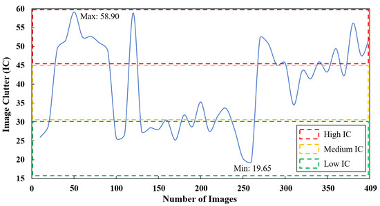
Figure 1.
The IC distribution of power line images.
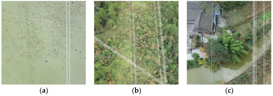
Figure 2.
Examples of power line images with different IC. (a) Low IC; (b) Medium IC; (c) High IC.
3. Power Line Extraction Method
The UAV image power line extraction method based on line detection and semantic segmentation proposed in this paper is mainly divided into three steps: (1) by combining the LSD algorithm and information entropy theory, an adaptive Gaussian pyramid multi-scale LSD algorithm is constructed, which can effectively extract the long and coherent line segment information in the image and form the power line candidate regions; (2) in order to reflect the interaction between line segments, an OMRF model on a WRAG is defined, in which the likelihood function is constructed by GMM, which utilizes the spectral and texture information of power lines, and the joint distribution is designed by considering the distance and angle between line segments, in order to realize pixel-level power line extraction; and (3) a simplified Kalman filter (KF) is used to track the power line pixels, in order to form a complete power line segment and eliminate the object fracture problem caused by image segmentation. Finally, the tracked power line pixels are fitted using the least-squares method. The specific technical process is shown in Figure 3.
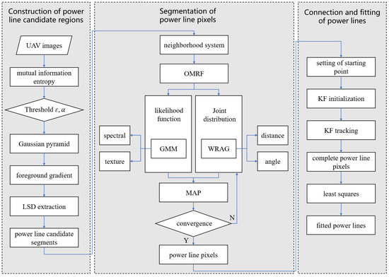
Figure 3.
Technical flow chart of power line extraction.
3.1. Construction of Power Line Candidate Regions
Due to the complex background of the image, it is impossible to directly extract the power line using the semantic segmentation algorithm. Considering the very prominent line structure, a line detector can be used to extract the line segments in the image first, in order to determine the power line candidate regions, which can effectively reduce the difficulty of subsequent segmentation and greatly improve the efficiency and accuracy of extraction. Commonly used line detectors include the Hough transform [23,24], Radon transform [25,26,27], and LSD [28,29,30], but the detection results of the first two methods are straight lines after fitting, and there is no pixel information of the original object; as such, they are not suitable for extracting candidate regions. LSD is a common and fast line detection method and the extracted results are straight line segments, which can be used to construct power line candidate regions with width information.
3.1.1. LSD Algorithm
Based on the gradient direction and amplitude of each pixel, LSD forms the regions of pixels that meet the constraints (determined through constraint rules) and generates line support regions as candidates for line segment detection. By the minimum constraint rule of the line support regions, whether the line support region is a line segment can be determined [28]. The algorithm only judges whether there are pixels with similar gradient angles through the neighborhood of one pixel; thus, it is easy to produce discontinuous line segments, and a large number of false line segments will be extracted in regions with dense vegetation, such as crops and forests. Therefore, the original LSD needs to be improved, in order to make this method more suitable for the construction of power line candidate regions.
3.1.2. Multi-Scale LSD Algorithm
In order to avoid the problem of line segment discontinuity caused by LSD using a single pixel, an adaptive multi-scale LSD algorithm combined with the information entropy theory is proposed, realized by the use of a Gaussian pyramid [31,32,33], which can mine the image information of the same object at different scales. In the process of building the image pyramid, Gaussian blur is applied to the image. If the image is blurred many times, the originally independent objects may be connected together, resulting in image distortion. If the algorithm detects a line segment in the distorted image, the result will also contain incorrect information; however, when there are too few images, the pyramid will lose information at a certain scale. Therefore, it is particularly important to determine the number of groups for the Gaussian pyramid and the number of images in each group.
Mutual information entropy can describe the similarity between two images. With this characteristic, the mutual information entropy between the Gaussian blurred image and the original image is calculated, and the results are compared with the threshold to determine whether to retain the processed image to construct an adaptive Gaussian pyramid, such that the algorithm can adapt to different image backgrounds. The calculation formula for the mutual information entropy is as follows:
where A and B are two images; a and b are image values; and are the information entropies of A and B, respectively; is the combined information entropy; and is the mutual information entropy.
The calculation steps can be summarized as follows: (1) Set l as the group of the adaptive Gaussian pyramid P, i as the image number in l, and initialize i and l = 0. (2) Take the input image a as the image i in group l; that is, the image at the bottom of P. (3) Use Gaussian blur for the image i of l and calculate . If < ε0, i = i + 1, and i is stored in the ith position of l; if > ε0, i is discarded and the construction of l is stopped. (4) Down-sample the i of l and calculate . If < α, l = l + 1, and i is stored in the ith position of l. Repeat (3)–(4) until > α. Then, i is discarded and the construction of P is stopped. (5) The P corresponding to image a is obtained.
The structure of the obtained P is shown in Figure 4. P has l + 1 groups, and the number of images in each group is uncertain; namely, i0 + 1, i1 + 1, i2 + 1, …, il + 1. The image in the group is obtained by Gaussian blurring the previous image of the current group, and the first image of the next group is obtained by down-sampling the last image of the previous group.
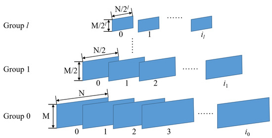
Figure 4.
Gaussian pyramid in multi-scale LSD.
3.1.3. Separation of Image Background
There is a lot of noise in the image background in the constructed adaptive Gaussian pyramid; however, the background is not important for the contour and edge of the object in the foreground. Therefore, it is necessary to separate the background from the foreground before line detection. This operation can avoid calculating non-edge pixels and save computation time. It can also reduce noise interference and avoid the false detection of line segments. The Otsu threshold [34,35,36,37,38] can be used to determine the gray level that can maximize the inter-class variance between the foreground and background and obtain the segmentation threshold of the foreground and background. The calculation formula is as follows:
where is the ratio of the number of foreground pixels to the total number of image pixels, is the average gray value of foreground pixels, is the ratio of the number of background pixels to the total number of image pixels, and is the average gray value of the background pixels.
When the background pixels in the image are similar, the original Otsu threshold algorithm has a better effect. When there are several kinds of background values in the image, the original Otsu threshold algorithm cannot separate the foreground well. In this paper, the Otsu threshold is optimized, the image is divided into several parts, and the foreground and background are separated using a gradient threshold. The calculation steps are as follows:
- (1)
- Read an image i in P and calculate the gradient for i.
- (2)
- Determine the pixel points x of the peak of , convert the Cartesian coordinates of x into polar coordinates, count the collinear x, and fit the lines L through the least-squares method. Then, calculate the intersection X between L and divide i into several parts through X.
- (3)
- Calculate σ with Formula 7 for each part of i, respectively.
- (4)
- Separate the local foreground of i from the background through σ, and corresponding to the background pixel is discarded.
- (5)
- Judge whether i is the last image in P. If not, repeat (4)–(5); if so, end the algorithm.
- (6)
- Obtain corresponding to the foreground pixel of i in P.
The image background is separated and the foreground is retained through the above steps. The original LSD algorithm is used to find the line segment according to the gradient angle, and segments are verified by the Helmholtz criterion. All reserved segments are considered power line candidate regions.
3.2. Segmentation of Power Line Pixels
3.2.1. OMRF Model
MRF [39] is a probabilistic graphical model, which provides a statistical method to simulate the spatial context constraints of images. Therefore, it is suitable for capturing texture information and has been widely used for semantic segmentation. The classical MRF model is a pixel-based model. The MRF model further considers semantic segmentation at the object level. The OMRF model [40] first uses the basic segmentation method to segment the given image into some over-segmented regions. Then, the region adjacency graph (RAG) is constructed using these regions, and the OMRF model is defined on the RAG (see Figure 5).
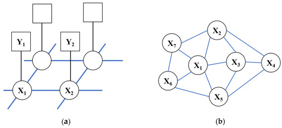
Figure 5.
Different types of MRF models. (a) Structure of the classical MRF model; (b) Structure of the RAG MRF model.
For image I, the OMRF model uses the basic unsupervised segmentation method to divide I into an initial region set R = {R1, R2, …, Rn}. Each Ri in R is an over-divided region (I = 1, 2, …, n), Ri ∩ Rj = Ø (i ≠ j), and n is the number of regions. Based on R, the OMRF model can construct an RAG G = (V, E), where V = (vi) is the vertex set and E = (eij) is the edge set. Each vertex vi represents an over-divided region Ri (I = 1, 2, …, n), and the existence of an edge eij indicates that the regions Ri and Rj are adjacent. Then, a label field X = {Xi|i = 1, 2, …, n} is defined on G. Each random variable Xi represents the class of region Ri, and takes a value in the set = {1, 2, …, }. Assuming that there are k different classes in I, let x = {xi|i = 1, 2, …, n} represent an implementation of X. In the OMRF model, the that maximizes the a posteriori probability distribution P(x|I) is regarded as the appropriate image segmentation result. The segmentation problem is transformed into the best implementation of estimating a given observed image I using the maximum a posteriori (MAP) criteria:
In Formula (8), the meaning of the MRF model defines the equation in the first line, and the Bayes formula provides the equation in the second line. As P (I) has no effect on the choice of x, the final equation can be defined.
The likelihood function P (I|x) is used to describe the conditional probability of image I belonging to the realization of x in the above equation, which can be further defined by GMM [41]. The feature vector of each random variable can be expressed as , where p is the dimensions of vectors. The parameters of GMM are the set of mean vectors of each class, µ = {µ1, µ2, ···, µk}, and the set of the feature covariance matrix of each class is = {1, 2, ···, k}, where k is the number of segmentation classes.
The joint distribution P(x) is used to simulate the spatial interaction between regions according to the label field. In addition, assuming that P(x) has the Markov property in the MRF model, it can be defined as:
where Ni is the set of regions adjacent to Ri. Based on the Hammersley–Clifford theorem [39], P(x) obeys a Gibbs distribution; that is:
where Z = is a normalized constant and U(x) = is an energy function, which adds the clique potential on all possible cliques C. In most cases of the OMRF model, only the pair-site cliques are used for the energy function, as they are simple in form but transmit context information.
3.2.2. Construction of WRAG
In the classic image segmentation RAG of the OMRF model, each vertex only indicates the existence of one region, and each edge only indicates whether two regions Ri and Rj are adjacent. However, the interactions between regions are complex, and the edge information in classic segmentation is not suitable for power line candidate regions; therefore, other information is required to measure the intensity of interaction. Therefore, a new WRAG, Gw (Vw, Ew), is constructed to describe the relationships between line segments, where the weights include the distances between line segments and the angle of line segments.
- (1)
- In order to reduce the amount of calculation and improve the calculation speed, OWRF adopts a neighborhood system for each object. The neighborhood is defined by the common boundary between the segment regions. However, for the problem of power line extraction, the detected segments are not necessarily adjacent to each other, and there is no complete common boundary, such that the neighborhood system cannot be defined with the boundary. In this paper, the k-nearest neighbors (kNN) method [42], based on the Euclidean distance, is used to construct the neighborhood system of line segments, where the value of k is 8. To obtain the distance, the line segments detected by multi-scale LSD are numbered (Figure 6). After numbering, each line segment L = {li|i = 1, 2, …, n} can be used to calculate the minimum Euclidean distance; that is:where x1, x2, y1, and y2 represent the abscissa and ordinate of any two points in the two segments, respectively. The neighborhood system after kNN clustering is shown in Figure 7. Neighborhood A, where segment L1 is located, includes another seven green segments close to L1, while segments of other colors belong to neighborhoods B, C, D, and E.
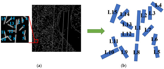 Figure 6. Numbered line segments. (a) Detection results of multi-scale LSD; (b) Number of local segments.
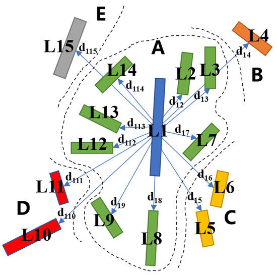 Figure 7. Neighborhoods of line segments.
 - (2)
- L in the above neighborhood system can be considered as the over-segmented region Rw = {|i = 1, 2, …, n} in WARP. The node VW = {|i = 1, 2, …, n} of each Ri represents a line segment. The edge set E can be replaced by the distance Ew between line segments; that is, Ew = { = dij|i, j = 1, 2, …, n}.
- (3)
- In addition to the distance between line segments, the angle between two lines also affects whether line segments can be classified into the same class. The angle α of a line segment can be calculated by using the two vertices A1 (x1, y1) and A2 (x2, y2) of the centerline of the line segment (Figure 8); the calculation formula is as follows:
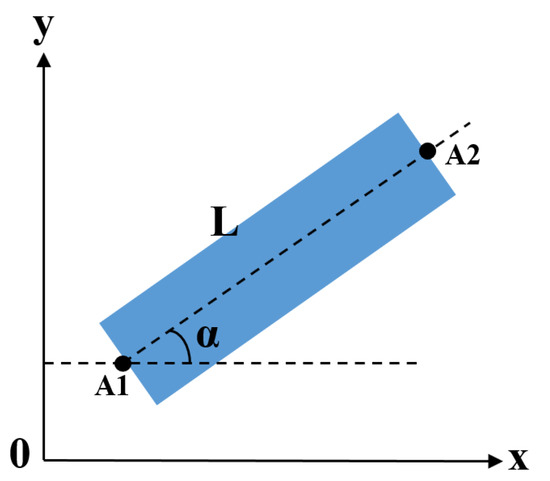 Figure 8. The angle α of a line segment.
From this, can be calculated; that is:
The range of is 0–180. When 0 < < 90, the greater the value of ∆α, the greater the included angle of the two line segments, and the smaller the weight represented by the angle. When 90 ≤ < 180, as the included angle increases, the two line segments tend to be parallel and the weight increases. Therefore, can be divided into the same increasing and decreasing trend, as in Formula (14): when approaches 0 and 180, increases.
- (4)
- If the RAG is directly constructed using line segments (Figure 9a), the adjacency relationship between each R is the same, and invalid line information cannot be eliminated. By calculating the minimum Euclidean distance and included angle between R, the WRAG, which includes the connection strength between line segments, can be defined (Figure 9b). Taking R1 as the calculation object, the adjacent line segments have different distances and included angles, such that they have different impact weights on R1.
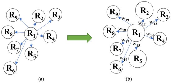 Figure 9. RAG and WRAG models. (a) RAG; (b) WRAG.
3.2.3. Definition of Likelihood Function
In the OMRF model, the likelihood function P (I|x) is equivalent to . IRi represents the feature vector of the object. In the image segmentation task, the feature vector often uses the spectral value of each pixel s in Ri. In this paper, the spectral and texture features of every pixel s in a power line segment Ri are combined with the GMM model to form a comprehensive feature vector IRi; namely:
where represents the spectral information of each pixel of the line segment, including the hue (h), saturation (s), and value (v) of the image; that is, = (h, s, v). represents the texture information of the line segment and the texture can be defined by information entropy; that is:
where n is the number of pixels in the line segment Ri, M and N are the image dimensions, and all pixels in one segment define the same texture.
In the meantime, assuming that the likelihood function conforms to a Gaussian distribution, can finally be written as:
where and represent the mean vector and covariance matrix of features in class h, respectively, which can be estimated using the maximum likelihood estimation algorithm; that is:
3.2.4. Definition of Joint Distribution for Label Field
Based on RAG information in the classic OMRF model, the clique potential Vc(x) of the joint distribution can be defined; for example, the commonly used multi-level logistic (MLL) model defines Vc(x) as:
The WRAG Gw(Vw, Ew) constructed in Section 3.2.2 improves the RAG and optimizes the lack of the interaction strength information between objects in the original model. Therefore, based on this WRAG, a new clique potential function Vw(xi, yi) can be proposed to measure the interaction between line segments. It is defined as:
where represents the angle information between line segments (the smaller the included angle between line segments, the greater the , and the greater the possibility of dividing segments into the same class) and represents the distance information between line segments (the greater the distance between line segments, the less likely they are to be divided into the same class).
Based on the proposed and Formula (10), the joint distribution can be written as:
The two weights and balance each other, as shown in Figure 10. R1–R9 are segments in the same neighborhood system, in which only R1, R2, and R5 are power lines and other segments are non-power lines. In the iteration, due to the large number of non-power lines around R1, the local probability of R1 being divided into non-power lines is very high in the original Vc(x). After introducing the angle weight, R1 and non-power line segments cannot be divided into the same class due to the large included angle between R1 and non-power line segments. However, if only the angle is used, R3 and R1 also have a small angle, such that they may be easily divided into the same class. This problem can be reduced by using the distance weight. R3 is far from R1 and, in fact, these two segments will not be divided into the same class (Figure 10).
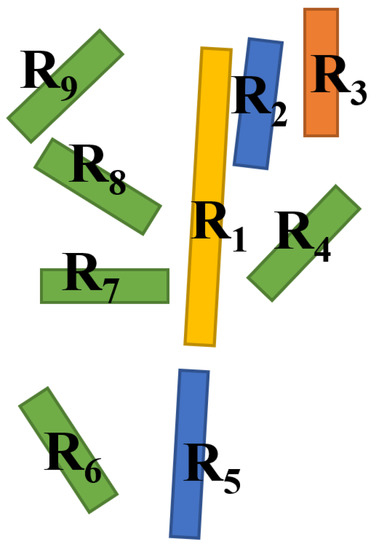
Figure 10.
The final segmentation results of power lines.
3.2.5. Maximum a Posteriori
The MAP criterion is used to iteratively optimize the results of the model (Formula (8)). There is no label field information in the first iteration, so the label field needs to be initialized. The k-means algorithm is often used as the implementation method of initialization in the MRF model. In the subsequent iteration, the tth posterior result is used as the (t + 1)th a priori hypothesis. The segmentation line, can be obtained by the MAP distribution criterion; that is:
According to this method, the pixels belonging to power lines can be obtained until the result converges. Some false extraction and interruption occur in the segmentation results, which require further processing to fit these line segments.
3.3. Connection and Fitting of Power Lines
The extracted power line pixels are often broken, and the extracted results need to be further connected to obtain a complete line. This paper uses the idea of the Kalman filter (KF) [43] and regards each disconnected power line segment as a uniform linear motion track. When the power line in a segment is interrupted, it is tracked to the next segment in a way similar to the KF. If there are segments that meet the matching conditions in the next segment, the segments are connected. After multi-scale LSD extraction and OMRF segmentation, there are few noise segments in the image. Therefore, the KF can be greatly simplified, only its tracking part is retained, and the filtering function is not considered. The KF consists of a state equation, a measurement equation, and a recursive iterative method. As there is no noise, the state equation for uniform motion is:
The measurement equation can be simplified to:
The state prediction equation in the system prediction stage is:
where and represent the state vectors at times k and k−1, respectively; represents the system state transition matrix; T is the step size; and represents the observation matrix. The state correction equation in the system update stage is:
After KF tracking and connection, the interrupted segments can be connected to form a more complete extraction result. Finally, the extracted power lines can be fitted directly, using the least-squares method. The specific steps are as follows:
- (1)
- Find the longest segment Rstart in the extracted segments Rextract, and take the midpoint of the Rstart centerline as the starting point x1.
- (2)
- Take the adjacent point x2 as the tracking direction point, and initialize the KF with the coordinates of x1 and x2.
- (3)
- Set the tracking step to n = 1.
- (4)
- Use the KF to track the next position and judge whether there is a point x3 of the line segment in the 8-neighborhood of x2.
- (5)
- If there is Rx3x2, add it to the tracked line segment, let x1 = x3, record the tracking position, and repeat step (3); if there is no Rx3x2, make n = n + 1, and judge whether N is greater than the preset step size or exceeds the image boundary. The preset step size is set to 20 pixels in this paper. The previous extraction method can obtain relatively complete power lines, and the fracture of the object is small. When it is more than 20 pixels, it is most likely that they are not interrupted power lines, but other false extraction results.
- (6)
- If n exceeds the step size, mark the segment as USED; if n does not exceed the step size, repeat step (4).
- (7)
- Judge whether all segments are marked as USED. If they are already marked, stop tracking and output all USED segments; if there are unmarked segments, repeat step (1).
- (8)
- All connected segments are fitted into straight lines using the least-squares method.
The flow of the method used in this paper is as follows. All experiments were designed and implemented using a PC with a Core i9-10850k CPU at 3.6 GHz with a 10 GB RTX3080 GPU and 128 GB of memory.
| Algorithm 1: Power line extraction algorithm based on multi-scale LSD and OMRF. |
| Input: Image I, information entropy thresholds α and ε, the number of classes k (k = 10 in this paper), potential function parameter β. |
Output: The power line extraction results.
|
4. Experimental Results
4.1. Analysis of Parameters
4.1.1. Thresholds of Multi-Scale LSD
As described in Section 3.1.2, two parameters are used when building the Gaussian Pyramid P: the threshold α is set as x times the normalized information entropy between the 0th image in group 0 and the 0th image in group 1 of P; and the thresholds ε0, ε1, …, εl are set as y times the normalized information entropy between the 0th image of the corresponding group and the 0th image of the 0th group of P. The specific values of x and y are determined experimentally.
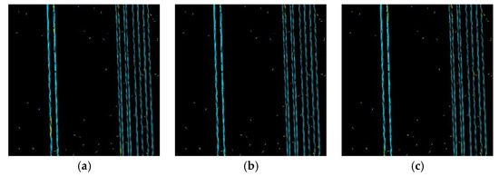
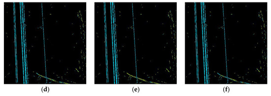
First, when the y value is not determined, y is temporarily set to 0.5. For the same input image, the x values are set to 0.4, 0.6, and 0.8, respectively. The typical detection results of a low IC image are shown in Figure 11a–f. Secondly, when the x value is not determined, x is temporarily set to 0.4. For the same input image, the y values are set to 0.5, 0.7, and 0.9, respectively. The typical detection results of a high IC image are shown in Figure 11g–l.
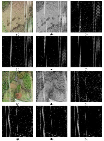
Figure 11.
Detection results with different thresholds in the multi-scale LSD. (a) Low IC image; (b) Gray image of (a); (c) LSD result of (a); (d) x = 0.4; (e) x = 0.6; (f) x = 0.8; (g) High IC image; (h) Gray image of (g); (i) LSD result of (g); (j) y = 0.5; (k) y = 0.7; (l) y = 0.9.
It can be seen that the multi-scale LSD combined with information entropy has more advantages than the original LSD algorithm in filtering short and small background segments, and has a strong ability to detect continuous and long segments. The power lines across the image are not easy to divide into multiple small segments, which can be used for line detection before further image segmentation. In terms of the threshold, with increases in x and y, the false detection of short line segments caused by land surface vegetation in the image background gradually decreases: with larger values of x and y, the fewer the number of images in the group corresponding to the input image, less detailed information of the image is retained, and the noise information in the background is filtered. However, if x and y are set too large, the power line segment will also be broken and discontinuous, while if x and y are too small, a large number of small line segments due to other objects in the background will appear, interfering with subsequent image segmentation. Through experimental testing, we determined the optimal values of x and y as 0.6 and 0.7, respectively. These thresholds give full play to the advantages of the Gaussian pyramid, not only ensuring that the power line segments will not be excessively split, but also filtering out a large number of noisy line segments of background objects, making it suitable for images with different IC.
4.1.2. Threshold β of OMRF
Before discussing the threshold β, it is necessary to select appropriate indices to quantify the performance of the segmentation algorithm. In this paper, pixel-level power line extraction is simplified into a binary classification problem. The class of power line pixels is the power line, and other background pixels are classified as non-power lines. Recall (Rec) and Precision (Prec) are used as evaluation indices, which are calculated as follows:
where TP represents the number of pixels whose detection result and the ground truth are both power lines, FP indicates the number of pixels detected as power lines but the ground truth is a non-power line, and FN is the detected non-power line where the ground truth is a power line. The higher the values of Rec and Prec, the more complete the extracted power line pixels are.
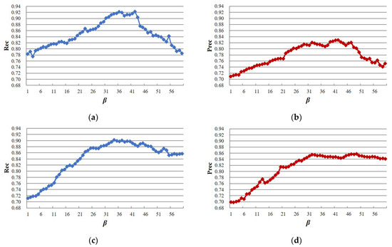
In the OMRF model, the parameter β in Formula (21) is very important and needs to be set manually. β is used to balance the influence between the likelihood function P (I|x) and the joint distribution P (x). A large value of β will emphasize P (x), and results with large uniform areas can be obtained; to the contrary, a small value of β will emphasize P (I|x), and results with many details will be obtained. Therefore, too large or too small β will lead to unsatisfactory results, and the β value is directly related to the size of the image to be segmented [44]. In order to analyze the influence of different values of β on the accuracy of power line segmentation, taking into account the size of images used in this paper, β was set the range 1–60 to segment the images, respectively.
The segmentation performance under different values of β is shown in Figure 12, from which it can be seen that when β = 20 and 60, the accuracy of power line segmentation is not as good as when β = 40. The interference of artificial features on the segmentation of power lines will be much greater than that for vegetation and bare land, and this phenomenon is more obvious when β is too small. The variation of the accuracy of the segmentation result is shown in Figure 13. When β increases, for different IC images, Rec and Prec have a similar trend—they first increase and then decrease, and finally, both will fall to a stable state. In the stage when Rec and Prec are increasing, P (I|x) and P (x) work together. At this stage, the energy of P (I|x) and P (x) gradually increases, the segments which have similar spectral and texture characteristics, a small distance from the power line, and a small included angle are gradually divided into one class, which means that more pixels are segmented into the true class. When β increases to a certain extent, the energy of P (I|x) becomes larger, the power line segments with similar characteristics but a long distance and large included angle may be divided into different classes, and the false and missed segmentation begins to increase. Therefore, there is a stage of Rec and Prec decline. In addition, the final stable accuracy for different IC images varies. This is due to the spectral fluctuation being small in low IC images, and the energy of P (I|x) mainly composed of spectral features is relatively small. In this state, when β increases, the energy of P (x) will far exceed that of P (I|x). Therefore, in the later iteration process, there will be more false detection and missed segmentation of images with low IC. In summary, we adopted β = 40 for the subsequent experiments in this paper; this value can ensure the high-accuracy extraction of power lines under different IC backgrounds.
4.2. Comparison of Different Methods
4.2.1. Results for Different IC Images
In this section, we discuss the power line extraction accuracy through KF tracking and fitting after multi-scale LSD detection and WRAG-OMRF segmentation and compare the results obtained by the proposed method with those of several common UAV image power line extraction methods. The selected comparison methods include: (1) the detection method based on the improved Hough transform (IHT) proposed by Li et al. [9], which uses knowledge-based line clustering to refine the detection results in the Hough space; (2) the cluster Radon transform (CRT) detection method proposed by Chen et al. [18], which uses the cluster index to enhance the anti-noise ability of the Radon transform; (3) the power line extraction method based on optimized LSD (OLSD) proposed by Ju et al. [45], which detects the object directly through the straight-line features of the power line; and (4) the original LSD and the original MRF (LSD-MRF) combined to form a simple detection method based on line detection and image segmentation.
The extraction results for each method are shown in Figure 14, Figure 15 and Figure 16. The results for the methods based on Hough and Radon were similar. The basic principle of these methods is to project the image space to a parameter space, and then select the peak points for straight-line fitting. Overall, IHT and CRT showed a good anti-interference effect on natural features such as water and vegetation. The short-edge features formed by these natural features will not be considered in the selection of peak points, such that the associated noise can be easily filtered. Note that IHT shows obvious fracturing of the power line with unclear edge features (Figure 14(a2)), while the straight lines fitted by CRT always run through the whole image (Figure 15(a3)), which do not form fractures due to the weakening of edge features and can effectively avoid the influence of highlighted roads. However, due to the difficulty of selecting the peak points of CRT, and judging and choosing the pixel characteristics on both sides of the power line, some chaotic false detection lines were generated (Figure 16(a3)). As it only considers straight-line features, OLSD cannot obtain good results. This method judges the background features as a large number of short straight lines (in particular, the leaves of vegetation have a great impact on them; see Figure 15(b4)), there are obvious misdetection results over roads with unclear straight-line features (Figure 15(a4)), and the anti-interference ability for artificial buildings is also weak; as such, it is only suitable for detecting power lines in images with a single background. After the line detection step, the classification is carried out using LSD-MRF, which can effectively filter out the background features, but there are also obvious fractures in the images with weak power line features (e.g., dense vegetation and highlighted roads; see Figure 15(a5,b5). The method proposed in this paper obtained satisfactory results, the extracted power lines were complete and accurate, and most kinds of ground objects in complex backgrounds could be effectively filtered; however, in some areas where the power line characteristics are not obvious and the intensity of background object characteristics is particularly large, false and missed detections may occur.
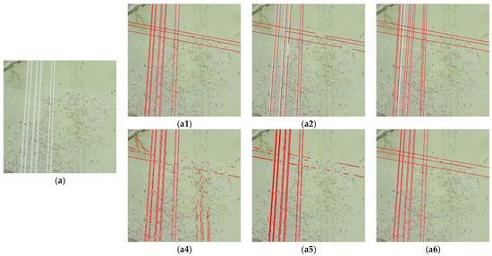
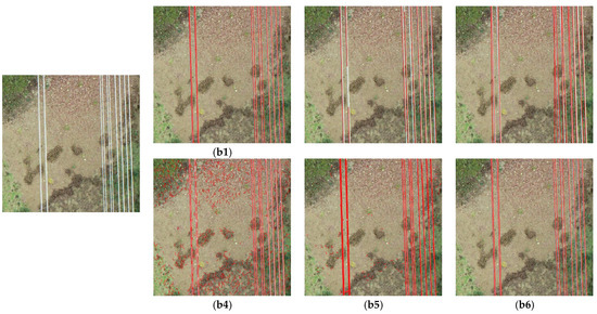
Figure 14.
Extraction results for low IC images: (a,b) are the original images; (a1,b1) are the ground truth; (a2,b2) are the results of the IHT method; (a3,b3) are the results of the CRT method; (a4,b4) are the results of the OLSD method; (a5,b5) are the results of the LSD-OMRF method; and (a6,b6) are the final fitting results of the method proposed in this paper.
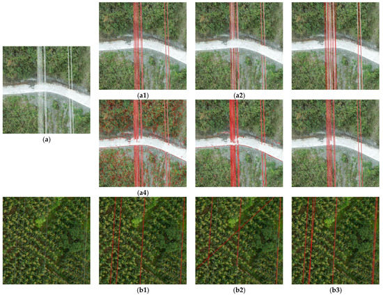
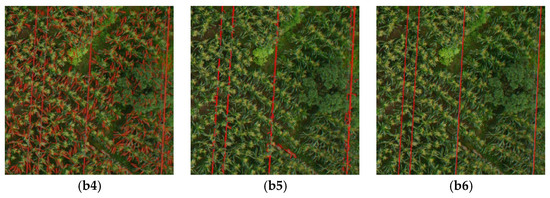
Figure 15.
Extraction results for medium IC images: (a,b) are the original images; (a1,b1) are the ground truth; (a2,b2) are the results of the IHT method; (a3,b3) are the results of the CRT method; (a4,b4) are the results of the OLSD method; (a5,b5) are the results of the LSD-OMRF method; and (a6,b6) are the final fitting results of the method proposed in this paper.
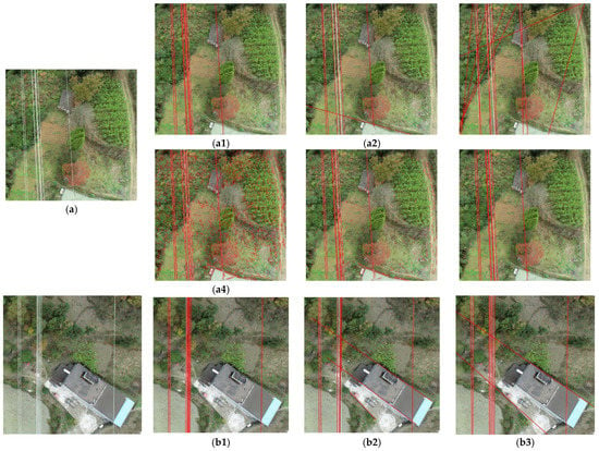
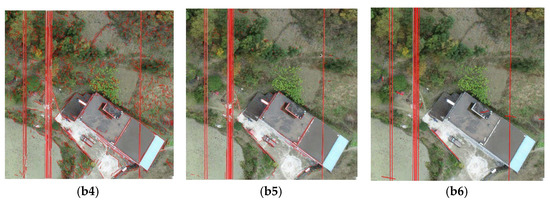
Figure 16.
Extraction results for high IC images: (a,b) are the original images; (a1,b1) are the ground truth; (a2,b2) are the results of the IHT method; (a3,b3) are the results of the CRT method; (a4,b4) are the results of the OLSD method; (a5,b5) are the results of the LSD-OMRF method; and (a6,b6) are the final fitting results of the method proposed in this paper.
The Rec and Prec values (Formulas (28) and (29)) were also used to compare the performance of the different methods; however, as some detection algorithms do not obtain power line pixel information, and the extraction results were only a fitted straight line, it was impossible to compare the accuracy by counting pixels. Therefore, the meaning of the variables in these formulas needed to be changed. Here, TP indicates that both the detection result and ground truth are the number of power lines, FN indicates that the background objects are misclassified into the detection results, and FP indicates that the detection result is the number of power lines but the ground truth is non-power lines. If the distance between the detected center point on the power line and the nearest point to the ground truth is less than 5 pixels and the angular deviation from the ground truth is less than or equal to 5°, it is considered that one power line has been successfully detected.
A total of 30 images were selected from low, medium, and high IC images in the data set for testing. The extraction accuracy values of the different methods for every test image are shown in Figure 17, and the average extraction accuracy for these images was also calculated (see Table 2). Overall, each method had relatively strong detection ability for low IC images, low accuracy for high IC images, and the influence of image background complexity on power line extraction was very obvious. The detection accuracy of IHT was close to that of CRT, and it had an acceptable extraction effect for images with simple backgrounds. The Prec of OLSD was low, the stability of this algorithm was not high, and there was no obvious correlation with the complexity of the background. The accuracy mainly depended on whether there were other objects with linear features in the image. The method used in this paper had high accuracy, with Rec up to 0.98 and Prec up to 0.97. The algorithm based on multi-scale LSD and OMRF with WRAG showed good performance for different IC images, and the stability of this method was strong.
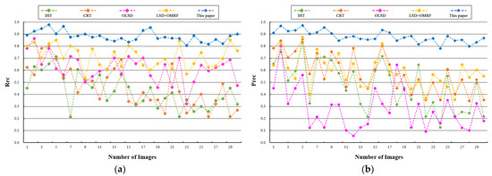
Figure 17.
The Rec and Prec values for different IC images. Abscissa values of 1–10 in the figures denote low IC images, 11–20 are medium IC images, and 21–30 are high IC images. (a) The Rec of test images; (b) The Prec of test images.

Table 2.
The mean Rec and Prec of test images.
4.2.2. Results of Images Including the Power Tower
In the power system corridor, there is always a symbiosis between the power line and the power tower. The power tower plays an important role in supporting and changing the direction of the power line. Therefore, the application of power line extraction methods in images including the power tower needs to be discussed separately. This section focuses on the comparison between the CRT algorithm and the method proposed in this paper. As shown in Figure 18, it can be seen that the addition of the power tower brings great challenges to the power line extraction task. The angle and direction of many parts of the power tower (e.g., the insulating ring) are consistent with that of a power line, and there are similar spectral and texture features of the power line in some tower areas. It is impossible to make an accurate manual judgment for some details, and boundary determination for the complete power line is fuzzy. The method based on the Radon transform fits the straight line by obtaining the peak points in the Radon field, where the straight line always runs through the whole image. Therefore, when the power tower changes the power line direction, the algorithm completely fails, cannot effectively display the difference in power line direction, and obtains a large number of false detection lines; however, the characteristics of the power tower itself have little impact on the CRT extraction results. The method used in this paper can resist the interference of the power tower, to a certain extent. Due to the manner of tracking pixels first and then fitting, the untraceable pixels do not participate in fitting, such that the straight-line objects can be segmented, which can accurately extract the power line and retain the power line direction difference at the same time; however, this method uses the pixel characteristics and object relationship of power lines, and false detection occurs in some areas with similar power line characteristics on the power tower.
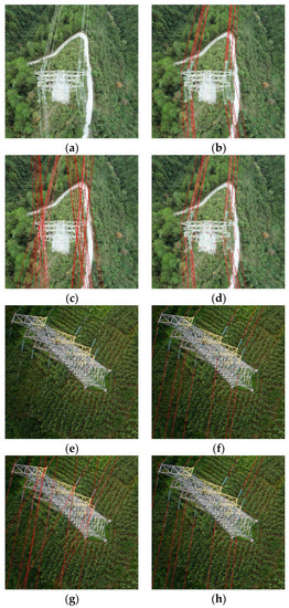
Figure 18.
Extraction results for images including power towers: (a,e) are the original images; (b,f) are the ground truth; (c,g) are the results for the CRT method; and (d,h) are the final fitting results for the method in this paper.
5. Discussion
- (1)
- The LSD algorithm is an efficient line detection method that can quickly obtain the line segments in an image. However, as the algorithm only judges whether there are other points with a similar gradient angle through the eight areas connected to one pixel, it is easy to produce discontinuous line segments, making it especially sensitive to noise, such as that associated with vegetation, and will produce a large number of short interference results. The multi-scale LSD algorithm used in this paper, combined with the information entropy theory and adaptive Gaussian pyramid, can effectively avoid the disadvantages of LSD and greatly improve the detection ability of LSD for continuous long lines. From the results, a large amount of vegetation information in the image background is filtered, the interruption of the detected straight lines is greatly reduced, and the complete extraction of long straight lines can be basically realized. Multi-scale LSD is more suitable as a line detection algorithm before power line pixel semantic segmentation and can reduce a lot of background noise to enhance subsequent operations.
- (2)
- MRF is a common machine learning algorithm in the field of image segmentation. Its main characteristic is the use of an undirected graph to represent the correlation between variables. It provides a simple way to visualize the structure of a probability model. In this paper, a GMM was used to define the likelihood function of the feature field, and the joint distribution of the label field was defined in combination with the idea of WRAG. This can effectively take into account the pixel information of the object on the image and the relationship information between objects, and form an effective OMRF model for power line pixel segmentation. The model has a strong information mining ability and can accurately segment power line and non-power line pixels, reduce the false lines (e.g., tree leaves and trunks) left by the line detection algorithm, and has good anti-noise ability for some objects with characteristics similar to power lines, such as the edges of artificial buildings. Compared with the method based on Hough and Radon, this method uses richer context information, rather than just edge information, and has a higher improvement in detection accuracy, especially for high IC images. Moreover, this method can obtain power lines in different directions, rather than the results always running through the image, which can be effectively used for extraction work with power towers and direction changes. Compared to the method using a single line detection algorithm, it avoids utilizing only the gradient changes on both sides of the power lines, reduces the influence of false lines from background objects, and improves the application ability of the algorithm in different scenes. This method can provide support for power line inspection work using UAV images with complex backgrounds.
- (3)
- The methods used in this paper also have shortcomings, including the following: With the deepening of the construction of the image feature and object relationship models, the complexity of the algorithm becomes higher and this kind of machine learning model requires a higher number of iterations, thus greatly reducing the efficiency of the algorithm, increasing the time cost of power line detection, and imposing higher computer hardware requirements. Therefore, it is not suitable for the fast or real-time detection of power lines. The statistical time cost results for different methods are shown in Table 3. Moreover, this algorithm lacks automation ability as a whole. Design parameters are required for multi-scale LSD and OMRF, and it is difficult or impossible to provide a suitable parameter value for various scenes, which means that the model may obtain unstable results when considering image data obtained in different situations. Subsequent research may consider designing the parameters to be adaptive, in order to deal with power line images with various complex environments. With the data accumulation and the further construction of data sets, deep learning and other AI methods will be applied for power line extraction from images, and the application and accuracy of extraction will be further improved by carrying out image fusion with other data, such as LiDAR point clouds.
 Table 3. Mean time cost on test images.
6. Conclusions
In this paper, a power line image data set was constructed using UAV images (with a total of 409 images) and the images were classified according to the background clutter. The data set contains power line objects with different specifications, rich background features, and diverse complexity, thus providing a reliable data basis for power line extraction algorithm research. In terms of methodology, the extraction of power lines was transformed into an image semantic segmentation task. A combination of multi-scale LSD based on adaptive Gaussian pyramid and OMRF with WRAG was used to obtain power line pixels. Finally, KF and the least-squares methods were used to track and fit power lines. The advantages of this method lie in two aspects: First, multi-scale LSD uses the multi-level information of the image to reduce the generation of background false line segments and is sensitive to long and continuous lines. The generated power line candidate regions can reduce the amount of noise, enhancing the subsequent segmentation. Secondly, OMRF uses segment distance and angle information to capture the complex interactions between segments by constructing WRAG. In order to simulate the interaction between line segments and obtain the characteristics of power lines, this information is further introduced into the joint distribution of the label field and the likelihood function of the feature field. OMRF with WRAG describes the interactions between objects through line information, which provides an optimized OMRF model for power line pixel segmentation. The experimental results for the test power lines from the proposed data set verified the effectiveness of this method. Compared with other power line extraction methods, the highest Prec value of this algorithm was 0.97, and the average Prec value for images with different IC was 0.88.
Author Contributions
Methodology, writing—original draft preparation, editing software, review, validation and formal analysis, W.Z. and Q.D.; investigation and data curation, Z.Z. All authors have read and agreed to the published version of the manuscript.
Funding
This research received no external funding.
Institutional Review Board Statement
Not applicable.
Informed Consent Statement
Not applicable.
Data Availability Statement
Not applicable.
Acknowledgments
We would like to give a special and heart-warming thanks to Beijing qzrobotics Technology Co., Ltd. (Beijing, China) for providing us with UAV imagery. A special acknowledgment should be expressed to the China-Pakistan Joint Research Center on Earth Sciences, who supported the implementation of this study.
Conflicts of Interest
The authors declare no conflict of interest.
References
- Sun, J.J. Application of GIS + GPS Intelligent Inspection System in Transmission Line Management. J. Anhui Electr. Eng. Prof. Tech. Coll. 2011, 3, 93–99. [Google Scholar] [CrossRef]
- Peng, X.Y.; Liang, F.X.; Qian, J.J.; Yang, B.; Zheng, X. Automatic Recognition of Insulator from UAV Infrared Image Based on Periodic Textural Feature. High Volt. Eng. 2019, 45, 922–928. [Google Scholar] [CrossRef]
- Van, N.; Nguyen, R.; Roverso, D. Automatic autonomous vision-based power line inspection: A review of current status and the potential role of deep learning. Int. J. Electr. Power Energy Syst. 2018, 99, 107–120. [Google Scholar]
- Berni, J.A.J.; Zarco-Tejada, P.J.; Suarez, L.; Fereres, E. Thermal and narrowband multispectral remote sensing for vegetation monitoring from an unmanned aerial vehicle. IEEE Trans. Geosci. Remote Sens. 2009, 47, 722–738. [Google Scholar] [CrossRef] [Green Version]
- Peng, X.Y.; Wang, K.; Xiao, X.; Wu, K.; Gu, W. Broadband Satellite Communication System in the Intelligent Inspection of Electric Powe Line Base on Large Scale Unmanned Helicopter. High Volt. Eng. 2019, 45, 368–376. [Google Scholar] [CrossRef]
- Zhou, Z.; Zhang, C.; Chen, X.; Fei, X.; Umer, T. Energyefficient industrial Internet of UAVs for power line inspection in smart grid. IEEE Trans. Ind. Inform. 2018, 14, 2705–2714. [Google Scholar] [CrossRef] [Green Version]
- Shan, H.T.; Zhang, J.; Cao, X.B.; Li, X.L.; Wu, D.P. Multiple auxiliaries assisted airborne power line detection. IEEE Trans. Ind. Electron. 2017, 64, 4810–4819. [Google Scholar] [CrossRef]
- Candamo, J.; Kasturi, R.; Goldgof, D.; Sarkar, S. Detection of thin lines using low-quality video from low-altitude aircraft in urban settings. IEEE Trans. Aerosp. Electron. Syst. 2009, 45, 937–949. [Google Scholar] [CrossRef]
- Li, Z.R.; Liu, Y.; Walker, R.; Ross, H.W.; Zhang, J. Towards automatic power line detection for a UAV surveillance system using pulse coupled neural filter and an improved Hough transform. Mach. Vis. Appl. 2010, 21, 677–686. [Google Scholar] [CrossRef] [Green Version]
- Wang, W.G.; Zhang, J.J.; Han, J.; Zhu, M. Broken strand and foreign body fault detection method for power transmission line based on unmanned aerial vehicle image. J. Comput. Appl. 2015, 35, 2404–2408. [Google Scholar] [CrossRef]
- Huang, X.; Zhang, Y.; Cheng, W.F.; Li, M.; Luo, B.; Zhou, K. Galloping monitoring method of transmission line based on image matching. High Volt. Eng 2015, 41, 808–813. [Google Scholar] [CrossRef]
- Chen, S.X.; Wang, B.H.; Sheng, G.H.; Wang, W.; Jiang, X.C. Application of digital image processing and photogrammetric technology to sag measuring method. High Volt. Eng. 2011, 37, 904–909. [Google Scholar] [CrossRef] [Green Version]
- Hao, Y.P.; Liu, G.T.; Xue, Y.; Zhu, J.; Lie, L. Wavelet image recognition of ice thickness on transmission lines. High Volt. Eng. 2014, 40, 368–373. [Google Scholar] [CrossRef]
- Shan, H.; Zhang, J.; Cao, X. Power line detection using spatial contexts for low altitude environmental awareness. In Proceedings of the 2015 Integrated Communication, Navigation and Surveillance Conference, Herdon, VA, USA, 21–23 April 2015. [Google Scholar]
- Yan, G.; Li, C.; Zhou, G.; Zhang, W.; Liu, X. Automatic extraction of power lines from aerial images. Geosci. Remote Sens. Lett. IEEE 2007, 4, 387–391. [Google Scholar] [CrossRef]
- Li, C.; Yan, G.; Xiao, Z.; Li, X.; Guo, J.; Wang, J. Automatic Extraction of Power Lines from Aerial Images. J. Image Graph. 2007, 12, 1041–1047. [Google Scholar] [CrossRef]
- Tan, J.S.; Guo, M. Automatic Extraction of Power Lines in Helicopter Power Line Inspection. Geospat. Inf. 2012, 10, 70–71. [Google Scholar] [CrossRef]
- Chen, Y.; Li, Y.; Zhang, H.; Tong, L.; Cao, Y. Automatic power line extraction from high resolution remote sensing imagery based on an improved radon transform. Pattern Recognit. 2016, 49, 174–186. [Google Scholar] [CrossRef]
- Zhang, J.; Shan, H.; Cao, X.; Yan, P.; Liu, X. Pylon line spatial correlation assisted transmission line detection. IEEE Trans. Aerosp. Electron. Syst. 2014, 50, 2890–2905. [Google Scholar] [CrossRef]
- Zhao, L.; Wang, X.; Yao, H.; Tian, M.; Jian, Z. Power line extraction from aerial images Using Object-based Markov Random Field with anisotropic weighted penalty. IEEE Access 2019, 7, 125333–125356. [Google Scholar] [CrossRef]
- Zhang, C.X.; Zhao, L.; Wang, Y.P. Research on fast extraction algorithm of power line in complex ground object background. Eng. J. Wuhan Univ. 2018, 51, 8. [Google Scholar]
- Song, B.; Li, X. Power line detection from optical images. Neuro Comput. 2014, 129, 350–361. [Google Scholar] [CrossRef]
- Song, X.Y.; Yuan, S.; Guo, H.B. Pattern identification algorithm with adaptive threshold interval based extended Hough transform. Chin. J. Sci. Instrum. 2014, 35, 1109–1117. [Google Scholar]
- Xu, Z.; Shin, B.S.; Klette, R. Accurate and robust line segment extraction using minimum entropy with Hough transform. IEEE Trans. Image Process. 2015, 24, 813–822. [Google Scholar] [CrossRef]
- Herumurti, D. Automatic urban road extraction on DSM data based on fuzzy ART, region growing, morphological operations and Radon transform. Proc. SPIE 2013, 8892, 88920A. [Google Scholar]
- Grigoryan, A.M.; Du, N. Comments on “Generalised finite Radon transform for N × N images”. Image Vis. Comput. 2011, 29, 797–801. [Google Scholar] [CrossRef]
- Kobasyar, M.; Rusyn, B. The Radon transform application for accurate and efficient curve. In Proceedings of the International Conference Modern Problems of Radio Engineering, Telecommunications and Computer Science, Lviv-Slavsko, Ukraine, 28 February 2004. [Google Scholar]
- Goio, V.; Jakubowicz, G.; Morel, J. LSD: A Fast Line Segment Detector with a False Detection Control. Pattern Anal. Mach. Intell. IEEE Trans. 2010, 32, 722–732. [Google Scholar] [CrossRef] [PubMed]
- Guo, K.Y.; Wang, Y.W.; Guo, X.L. Lane Classification Algorithm Combined LDA and LSD. Comput. Eng. Appl. 2017, 53, 219–225. [Google Scholar] [CrossRef]
- Liu, B.Y.; Zhao, Z.Y. Path Edge Recognition Strategy Based on Improved LSD and AP Clustering. J. Graph. 2019, 5, 915–924. [Google Scholar]
- Lopez, J.; Santos, R.; Fdezvidal, X.R. Two-View Line Matching Algorithm Based on Context and Appearance in Low-Textured Images. Pattern Recognit. 2015, 48, 2164–2184. [Google Scholar] [CrossRef]
- Sun, J.J.; Zhao, Y.; Wang, S.G. Improvement of SIFT Feature Matching Algorithm Based on Image Gradient Information Enhancement. J. Jilin Univ. Sci. Ed. 2018, 56, 82–88. [Google Scholar] [CrossRef]
- Wang, D.M.; Xie, X. Improved LSD Algorithm Based on Entropy Adaptive Gaussian Pyramid. J. Jilin Univ. Inf. Sci. Ed. 2020, 38, 9. [Google Scholar]
- Wang, Z.; Ge, B.; Tu, M.Y. Image Segmentation Algorithm Based on Improved Otsu Algorithm and Artificial Fish Swarm Optimization. Packag. J. 2019, 11, 81–86. [Google Scholar]
- Li, B.Y.; Fan, Y.G.; Gao, Y. Infrared Image Feature Extraction Based on Otsu and Canny Operator. J. Shaanxi Univ. Technol. Nat. Sci. Ed. 2019, 35, 33–40. [Google Scholar]
- Wang, X.; Yin, L.W.; Guo, X.X. Automatic power line extraction from high resolution remote sensing imagery based on an improved radon transform. J. Jilin Univ. Sci. Ed. 2018, 56, 179–184. [Google Scholar]
- Liu, K.P.; Li, X.W.; Li, Y. SIFT Image Matching Algorithm Based on Edge Information. J. Jilin Univ. Inf. Sci. Ed. 2018, 36, 91–97. [Google Scholar]
- Shen, X.J.; Qin, J.; Lu, Y.D. Fast Multi-Threshold Otsu Algorithm with Complete Linear Time Complexity. J. Jilin Univ. Eng. Technol. Ed. 2019, 49, 273–279. [Google Scholar] [CrossRef]
- Li, S.Z. Markov Random Field Modeling in Computer Vision, 3rd ed.; Springer: Berlin/Heidelberg, Germany, 2009. [Google Scholar]
- Zheng, C.; Yao, H. Segmentation for remote sensing imagery using the object-based Gaussian–Markov random field model with region coefficients. Int. J. Remote Sens. 2019, 40, 4441–4472. [Google Scholar] [CrossRef]
- Bilmes, J.A. A Gentle Tutorial of the Em Algorithm and Its Application to Parameter Estimation for Gaussian Mixture and Hidden Markov Models; Technical Report; International Computer Science Institute: Berkeley, CA, USA, 2000. [Google Scholar]
- Li, Y.; Hu, Z.; Gang, Z.L.; Sotelo, M.A. Image sequence matching using both holistic and local features for loop closure detection. IEEE Access 2017, 5, 13835–13846. [Google Scholar] [CrossRef]
- Wen, G.J.; Wang, R.S. A Robust Approach to Extracting Straight Lines. J. Softw. 2001, 12, 1660–1666. [Google Scholar]
- Zheng, C.; Wang, L. Semantic Segmentation of Remote Sensing Imagery Using Object-Based Markov Random Field Model with Regional Penalties. IEEE J. Sel. Top. Appl. Earth Obs. Remote Sens. 2015, 8, 1924–1935. [Google Scholar] [CrossRef]
- Ju, C.Y.; Shi, Y.; Gao, S.D.; Sun, B.Y. Power Line Extraction in Aerial Photogrammetry DOM Based on LSD Algorithm. Electr. Power Surv. Des. 2020, S02, 166–170. [Google Scholar]
Publisher’s Note: MDPI stays neutral with regard to jurisdictional claims in published maps and institutional affiliations. |
© 2022 by the authors. Licensee MDPI, Basel, Switzerland. This article is an open access article distributed under the terms and conditions of the Creative Commons Attribution (CC BY) license (https://creativecommons.org/licenses/by/4.0/).
