
Accuracy Assessment, Comparative Performance, and Enhancement of Public Domain Digital Elevation Models (ASTER 30 m, SRTM 30 m, CARTOSAT 30 m, SRTM 90 m, MERIT 90 m, and TanDEM-X 90 m) Using DGPS


Abstract
1. Introduction
Vertical Accuracy of DEMs
2. Study Area, Data and Methodology
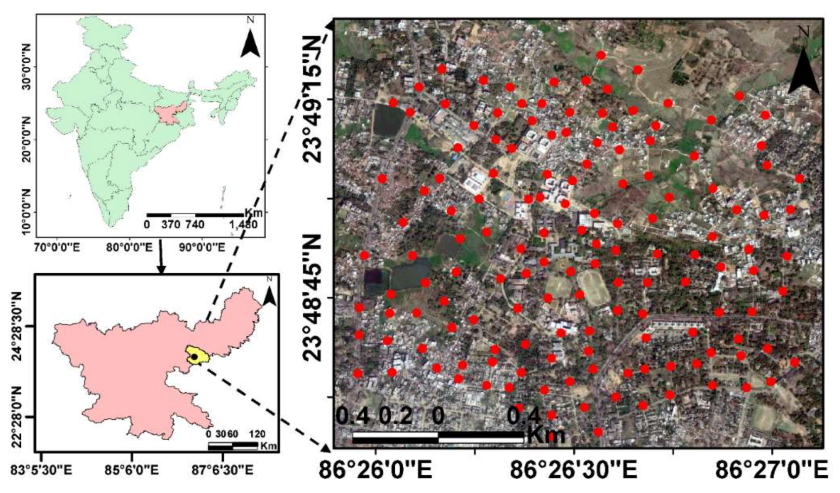
2.1. Study Area
2.2. Data
2.2.1. Satellite/Space Shuttle Derived Digital Elevation Model (DEM) Data
ASTER DEM
SRTM DEM
Cartosat DEM
MERIT DEM
TanDEM-X DEM
2.2.2. Ground Observation-Based Data
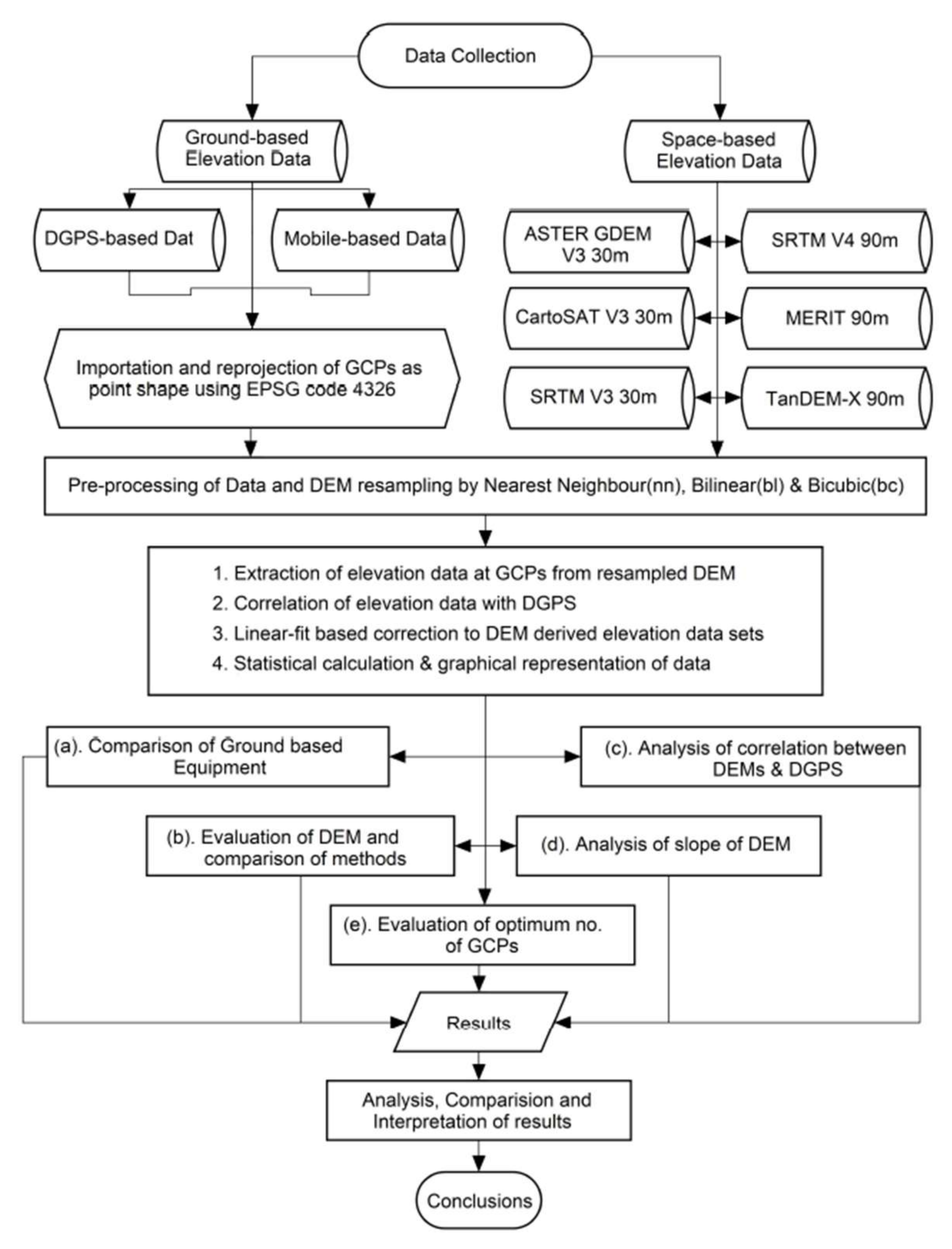
2.3. Methodology
2.3.1. Statistics
2.3.2. Statistical Analysis, Correlation Statistics, Tests and Optimum Number of GCPs
2.3.3. Correction of DEMs Using DGPS Data
3. Results and Discussion
3.1. Descriptive Statistics and Comparison of Ground-Based Equipment (DGPS and MobileGPS)
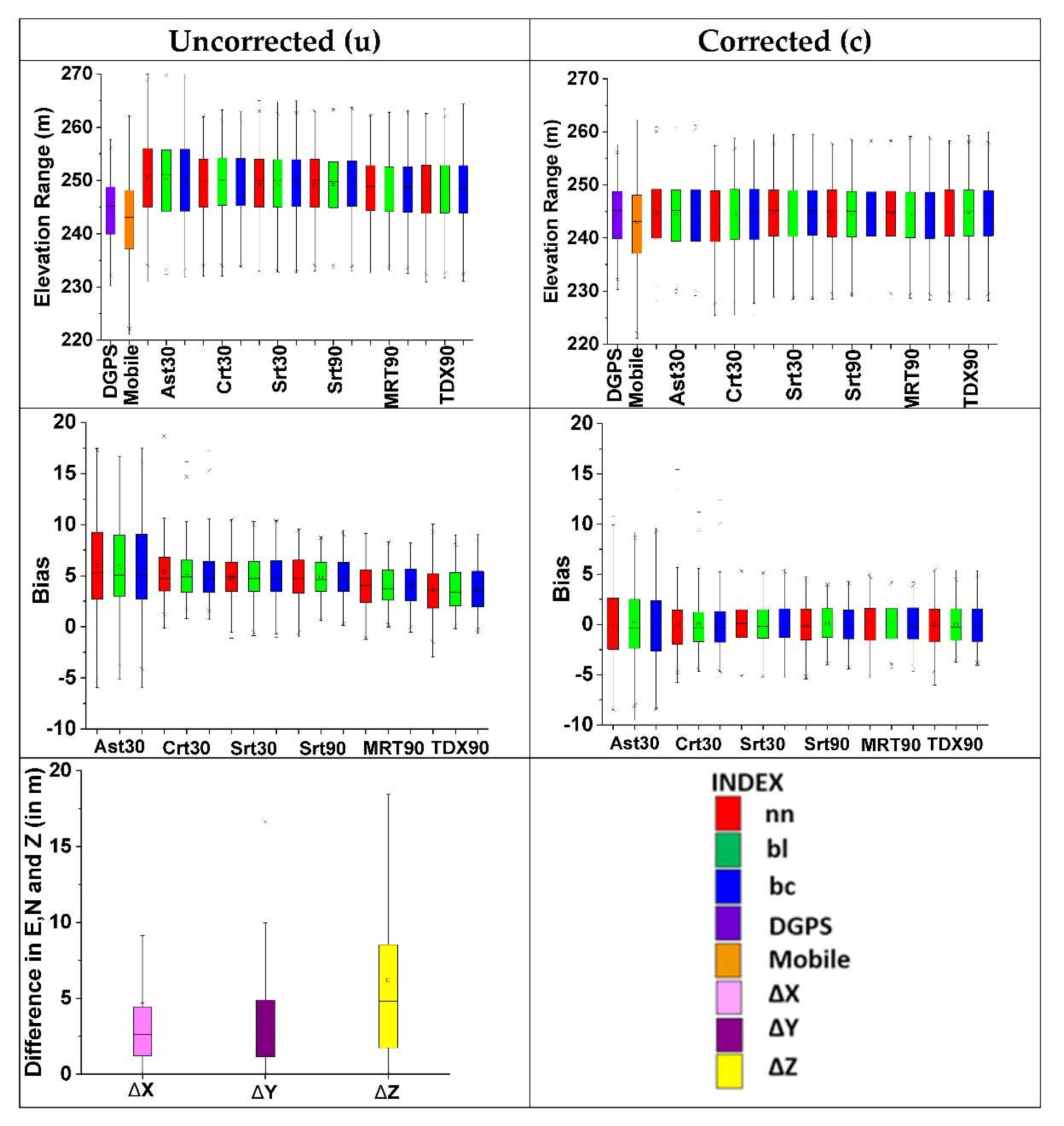
- The boxplots exhibit the changes observed in the elevation range and bias before and after correction of DEMs using DGPS values (Figure 3).
- The descriptive statistics of DGPS and MobileGPS (Table 3) show that MobileGPS has a higher SD, RSD (%), and SE as compared to DGPS for the elevation (Z) measured at GCPs. The MBE (in m) shows that the mean bias error shown by MobileGPS with respect to DGPS is in the range of meters. For instance, the underestimation of elevation by MobileGPS is −1.32 m compared to DGPS.
- The correlation statistics show poor correlation between elevation estimates obtained from DGPS and MobileGPS (r2 = 17.45%) (Table S2).
- The differences in values of positional attributes (ΔX, ΔY, ΔZ, shown in the lower panel) observed at GCPs by DGPS and MobileGPS are shown in Figure 3.
- The mean bias error (MBE) for the positioning attributes (MobileGPS–DGPS) observed at GCPs was found to be relatively poor (0.49 m, 1.43 m, and −1.32 m for easting (E), northing (N), and elevation (Z), respectively) (Table 3).
- The root mean square error (RMSE) for the positioning attributes (MobileGPS–DGPS) observed at GCPs was found to be relatively poor (10.10 m, 5.02 m, and 8.93 m for easting (E), northing (N), and elevation (Z), respectively) (Table 3).
- The mean absolute error (MAE) for the positioning attributes (MobileGPS–DGPS) observed at GCPs was found to be relatively poor (4.59 m (ΔX), 3.56 m (ΔY), and 6.21 m (ΔZ) for easting (E), northing (N), and elevation (Z), respectively) (Table 3).
- Therefore, DGPS estimates at GCPs have been used as a reference dataset for further comparison with space-based DEMs as MobileGPS gives relatively poor estimates of elevation, as mentioned above.
3.2. Comparison of DEMs with Respect to DGPS Estimates
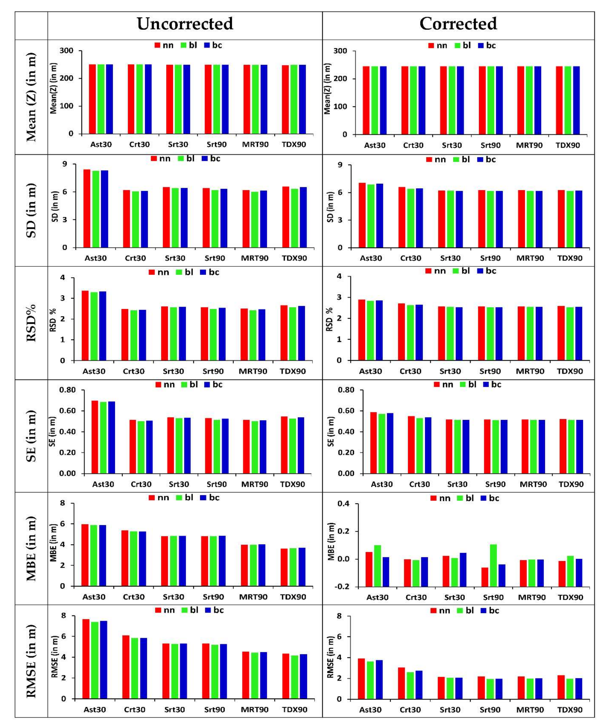
3.2.1. Mean Elevation (Mean (Z))
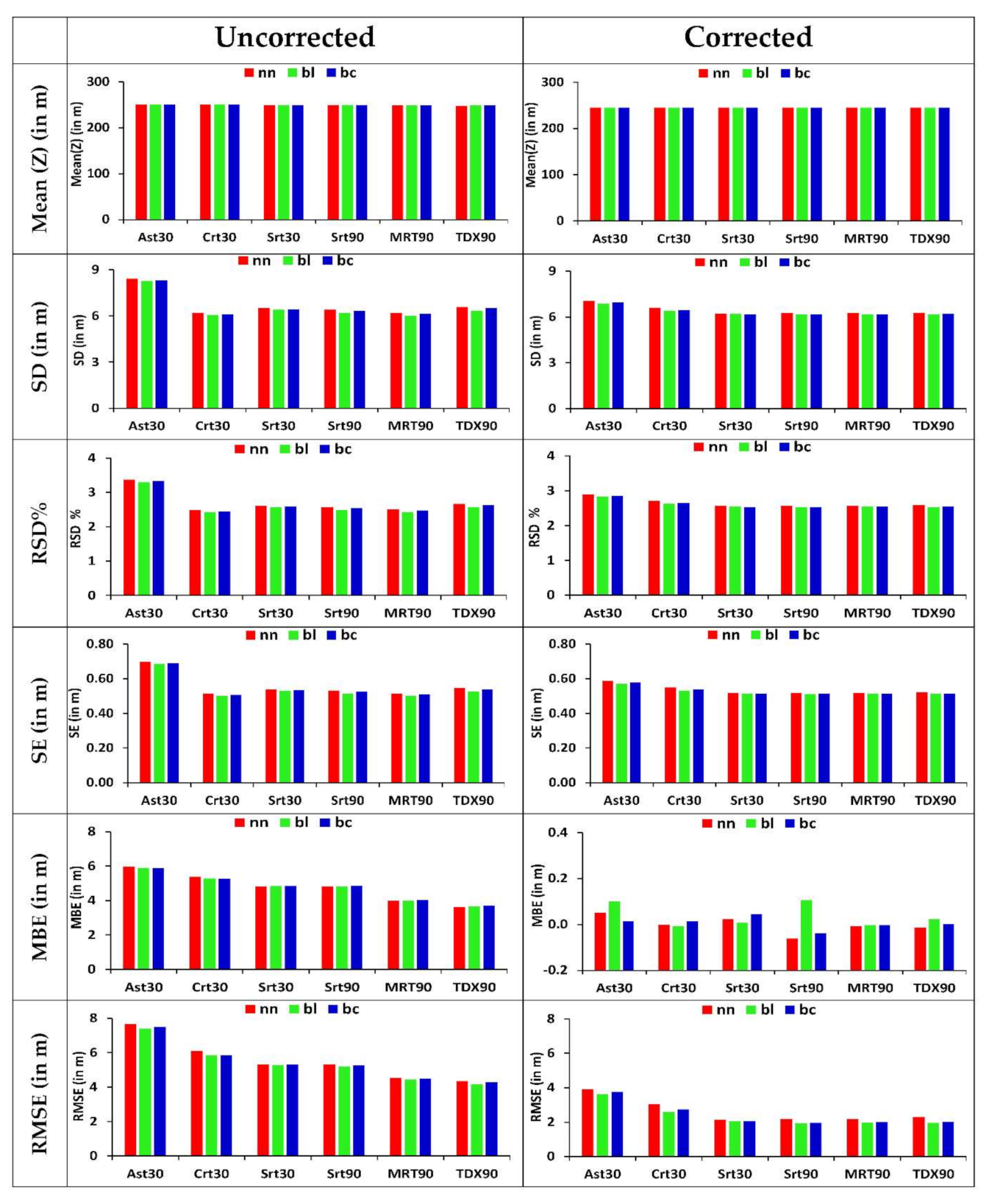
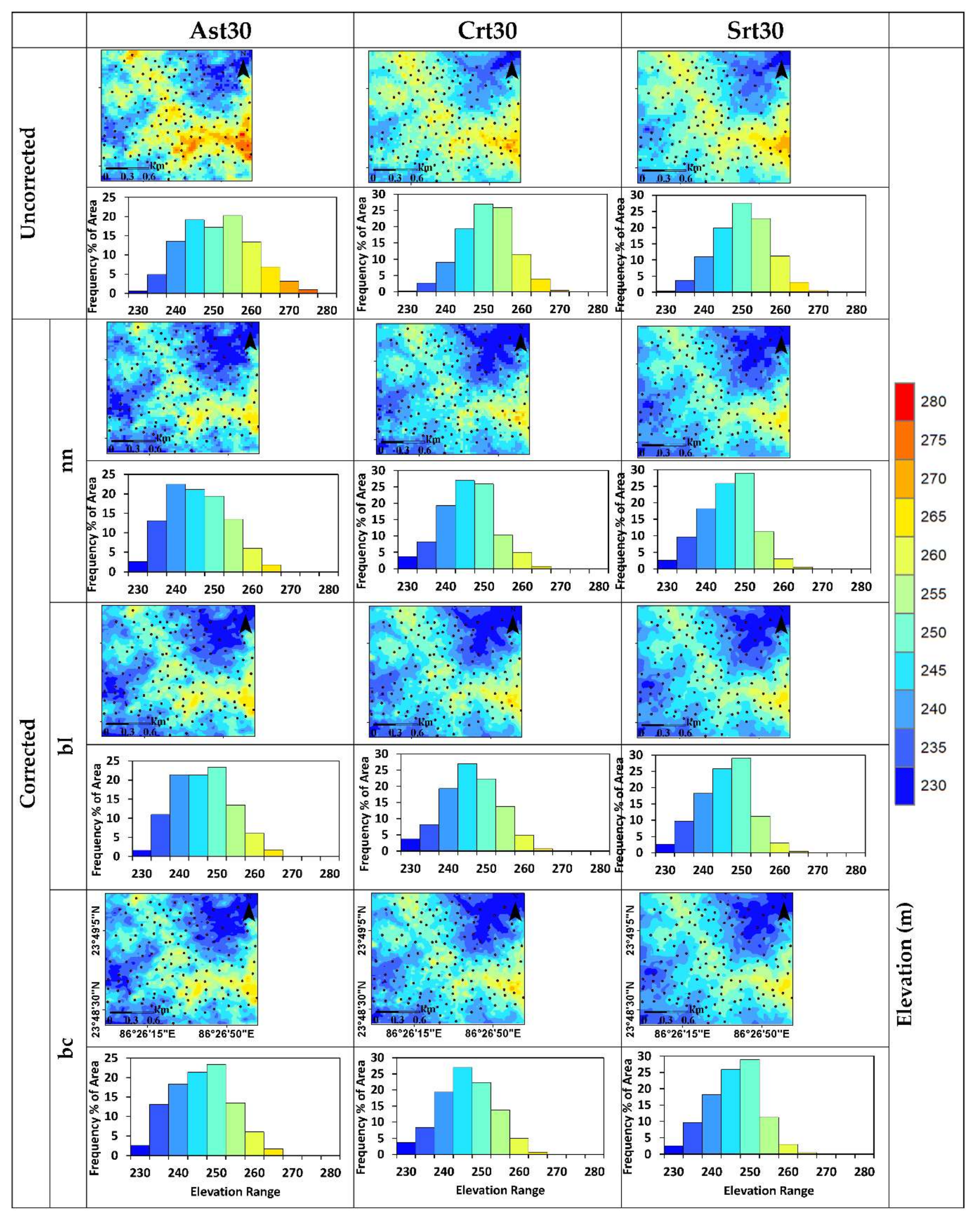
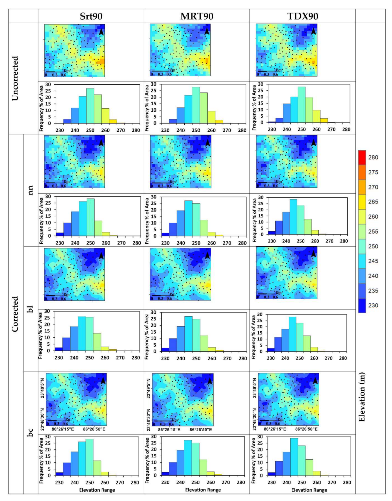
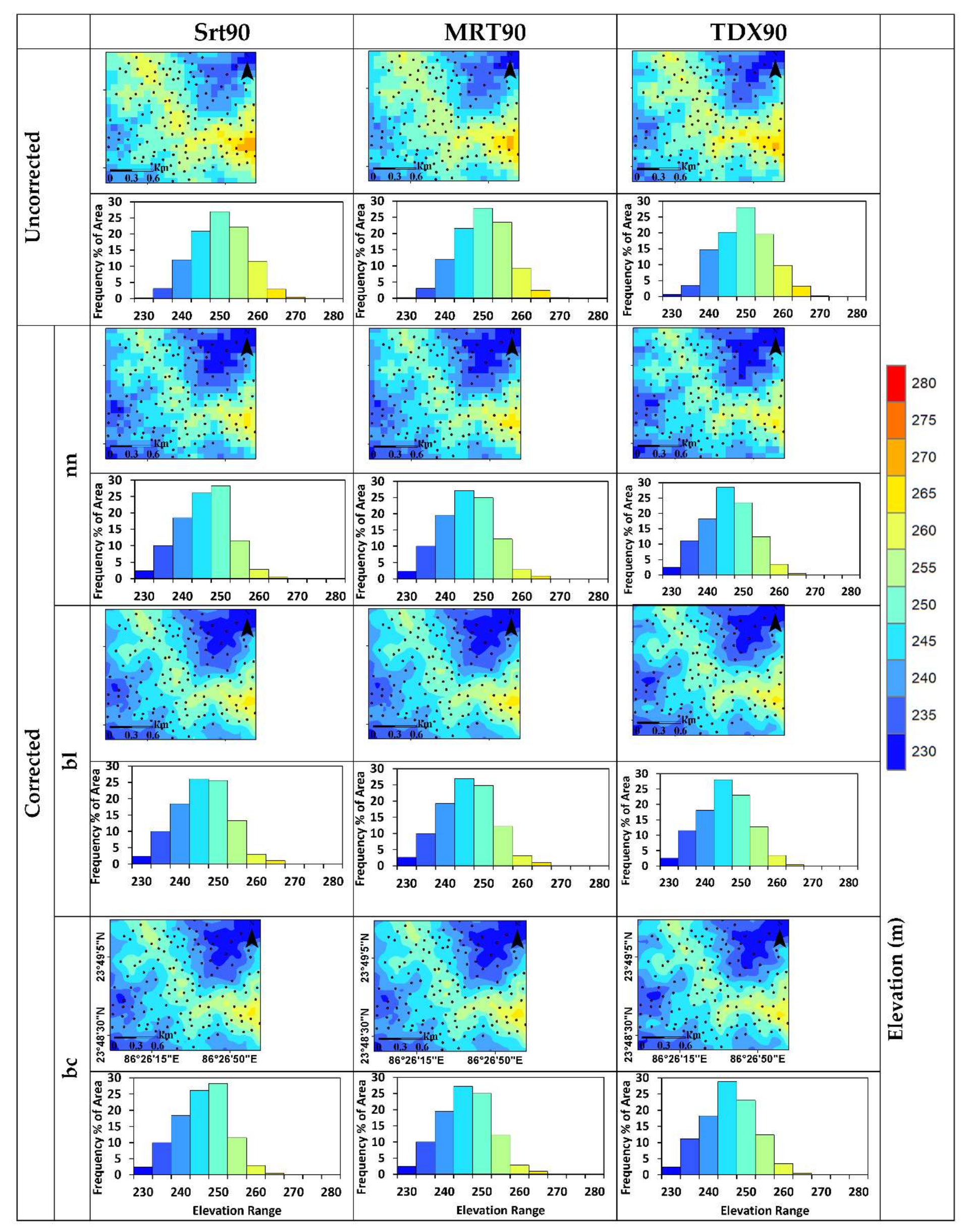
- The average elevation was found to be varying between 248.03–250.37 m in the uncorrected (original) elevation datasets.
- After correction, all DEMs (ASTER, CARTOSAT, SRTM, MERIT, and TanDEM-X) show consistency in the elevation values, with only negligible differences due to the interpolation methods (nn, bl, and bc).
- As the elevation values obtained from the corrected DEMs are found to be consistent with respect to the reference dataset (DGPS), it is recommended that DEMs need to be corrected using DGPS estimates over GCPs before being used in any scientific studies.
- The pairs of elevation values from the corrected and uncorrected DEMs were also tested for any significant difference using a paired t-test at 99% CL & α = 0.01 (Table S3). The elevation estimates from DEMs, before and after correction (uncorrected vs. corrected), were found to be significantly different for all cases (nn, bl, and bc).
- It is notable that the two-tail F-test for finding the differences in the variances of elevation values (at 99% CL & α = 0.01) using uncorrected (u) and corrected (c) DEM rasters were found to be insignificant (Table S4). This implies that the variances of these two datasets (uncorrected and corrected DEMs) are similar.
- These statistical tests emphasize the usefulness of the correction of DEMs using DGPS values.
- The two-tail paired t-test for the hypothesized mean difference of the elevation (Z) values (at 99% CL & α = 0.01) was carried out taking pairs of elevation values observed by DGPS and sampled over (corrected/uncorrected) DEM rasters to test whether the difference in the mean of elevation before and after the correction was significant or not with respect to DGPS (Table 8 and Table 9). The elevation estimates from DGPS and DEMs were found to be significantly different before applying correction (Table 8), whereas they turned out to be insignificant after correction.
- Similarly, two-tail F-test for the variances of the elevation values (at 99% CL & α = 0.01) were carried out between DGPS and DEMs (uncorrected or corrected) (Tables S5 and S6). The differences in the variances of these two pairs were found to be insignificant, that is, the variances of these two datasets (DGPS and DEMs (uncorrected or corrected)) were similar.
3.2.2. Measure of Dispersion (Standard deviation (SD), Relative Standard Deviation (RSD) and Measure of Eror (Standard Error (SE))
- The SD/RSD/SE values for the bilinear method show lower values compared to other interpolation methods for all DEMs, and also for uncorrected and corrected datasets.
- After correction, the percent change in SD for DEMs is observed to be variable. The percent change in SD for the Ast30, Crt30, Srt30, Srt90, MRT90, and TDX90 datasets is −16.43%, −6.07%, −3.72%, −1.80%, 1.51% and −3.97%, respectively (Table 6). A similar percent change was observed for SE (Table 6). Ast30 shows a considerably higher percentage change in SD/SE, after correction, compared to other DEMs.
3.2.3. Measures of Systematic Error (MBE) and Magnitude of Errors (RMSE and MAE)
- The measures of error were found to vary for different DEMs and interpolation methods. The RMSE for uncorrected datasets was found to be between 4.17 and 7.65 m, while MBE and MAE were found to be falling within the range of 3.62–5.96 m and 3.66–6.35 m, respectively.
- After correction, there was a substantial reduction in bias (MBE), which was also reflected in the RMSE and MAE values (Figure 4, Table 4). The reduced range of RMSE and MAE was 1.91–3.91 m and 1.59–3.11 m, respectively. The MBE was reduced to nearly zero after the correction. The amount of error reduction is visible in the form of a percent decline in the RMSE, MBE, and MAE values (Table 6). The percent decline in RMSE due to correction is observed to be nearly 50–62%, whereas this reduction is about 99–100% for MBE and about 50–65% reduction in MAE. Such a reduction in RMSE achieved using linear fit correction of DEMs is less than the 91% to 93% reduction in RMSE achieved using the back-propagation neural network (BPNN) technique [91].
- Our results for MRT90 show an average RMSE value, including all three resampling methods (nn, bl, and bc), which show ranges of 4.49–5.54 m before correction and 1.99–2.18 m after correction (Table 4). The average RMSE, before (4.49 m) and after correction (2.05 m), falls well within the expected accuracy of 12 m reported by product specification [68], and even shows a much lower average RMSE than previous findings [79,80].
- The average RMSE value of the nn, bl, and bc techniques obtained for TDX90 in this investigation is: before (4.26 m) and after (2.09 m) correction. This falls well within the expected accuracy range of 10 m [70] and shows a considerably lower value of RMSE for the corrected DEM, as reported by other researchers [74,80]. The MAE (3.69 m before and 1.73 m after correction) and MBE (3.65 m before and nearly zero after correction) as observed for TDX90 reflect the quality of the product, even showing lower values than those obtained for the Indian region [79]. The lower values of MAE and MBE in this case may be attributed to relatively planar topography compared to the moderate and rugged topography from the previous findings.
- The average RMSE value observed for CartoDEM in both cases (before correction, 5.93 m, and after correction, 2.78 m (Table 4)) meets the product specification RMSE value of 8 m [64,66]. The RMSE value after correction shows a lower value compared to previous studies [40,93]. However, it is slightly higher than 1.96 m, as reported by another study for a plain area [79].
- Among the 30 m elevation datasets, Srt30 shows a relatively lower value of RMSE, MBE, and MAE, both before and after correction, and performs better than the other two DEMs (Ast30 and Crt30)—followed by Crt30 (Table 4).
- On the other hand, among the 90 m elevation datasets, TDX90 shows better performance before correction, as indicated by its lower RMSE, MBE, and MAE values, while after correction, all the datasets (Srt90, MRT90 and TDX90) are exhibiting similar performance with consistent RMSE, MBE, and MAE values with negligible differences (Table 4).
- Overall, the Ast30 dataset shows a relatively poor performance in both cases—before and after correction. This can be seen in the relatively higher values of RMSE/MBE/MAE (Table 4). Similar results have been obtained by many researchers for the older version of Aster GDEM [51,73,80,94,95]. The results obtained for the latest version of ASTER GDEM (ASTER GDEM version 3) in this study agree well with recent investigations for this latest version [96].
- Despite the coarser resolution, TDX90, before correction, exhibits considerably lower RMSE/MBE/MAE values compared to the rest of the DEMs (ASTER GDEM, CartoDEM, SRTM, and MERIT DEM) utilized in this study.
- Though the differences arising from the interpolation methods can be considered to be negligible for all DEMs, the RMSE values are relatively lower for the bilinear method—both before and after correction (Table 4).
- The impact of the correction of DEMs using DGPS values is visible in the form of the substantial reduction of error (RMSE/MBE/MAE).
- The better performance of TDX90 can be attributed to data collection and processing techniques. The elevation data were derived by single pass SAR (Synthetic Aperture Radar) interferometry using pairs of SAR images, which were acquired during the four-year period of between December 2010 and January 2015 [71] by the twin satellites in bistatic mode (TerraSAR-X and TanDEM-X). The landmasses with complex topography were covered at least twice, which involved the repositioning of orbits in order to avoid the shadowing effect in rugged/mountainous terrain [71,97,98].
- As both Ast30 and Crt30 have been generated through optical stereoscopy, the better accuracy obtained for Crt30 over Ast30 can be attributed to CartoDEM’s generation technique and the finer spatial resolution of the input data. CartoDEM is created using high-resolution (2.5 m) optical stereoscopic imaging, which can capture topographic differences at a finer scale. The ASST (Augmented Stereo Strip Triangulation) technique was used to create the CartoDEM, which included very precise ground control points, interactive cloud masking, and automatic dense conjugate pair generation using aspect-based correlations to determine the best match point [66]. In stereo-pairs, aspect-based correlation is particularly effective and efficient [99].
3.2.4. Bias (DEM-DGPS)
- The bias before correction, which is observed for different DEMs, is found to show variation that ranged between 3–6 m. The lowest average bias among 30m datasets is observed for Srt30 (4.82 m). On the other hand, TDX90 (3.65 m) shows the lowest bias among the 90 m datasets (Figure 3, Table 7)). After correction, all DEMs show nearly zero bias, which can also be observed in the percent reduction in MBE after correction (Table 6).
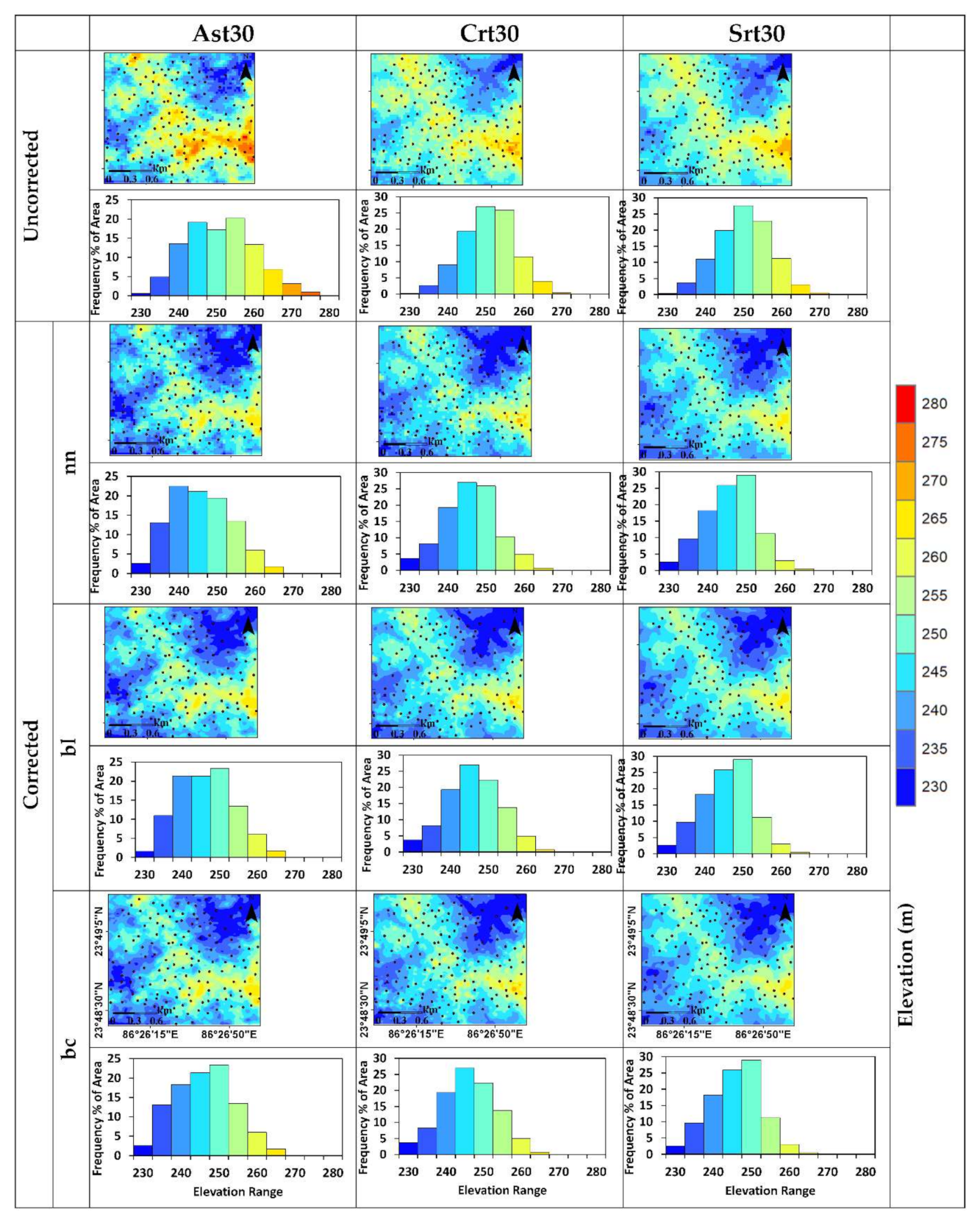
- In the Bias vs. Slope chart (Figure S1), the uncorrected datasets show the systematic nature of bias while the corrected datasets show a random distribution of bias. The removal of systematic bias using DGPS values can help in the reduction of associated errors. Therefore, after the correction of DEMs, a substantial improvement in bias is visible compared to uncorrected DEMs. This underlines the importance of applying correction to DEMs using DGPS estimates. The improvement is also visible in the spatial distribution of bias in elevation (between corrected and uncorrected DEMs) in the form of a map and corresponding histogram (Figures S2 and S3).
3.3. Slope
- The elevation datasets with a coarser resolution (Srt90, MRT90, and TDX90) were found to show lower average slope values compared to datasets with relatively finer resolution (Ast30, Crt30, and Srt30) (Table 10), which is expected for a coarser resolution dataset (at 90 m vs. 30 m DEMs).
- For all DEMs, the slope values (average, minimum, and maximum) show a marginal drop in values before and after the correction (Table 10). The smoothening over a larger area had led to lower slope values in Srt90 compared to Srt30. Therefore, for ground flow modelling, which is directly dependent on slope values across different directions, Srt30 is preferable over Srt90. Thus, it can be concluded that for surface ground flow modeling, finer resolution datasets are preferable over coarser ones.
- From the paired t-test for the means of the slope values (at 99% CL & α = 0.01) for all DEMs, it is observed that the change in slope values (before and after correction) is significantly different (Table S7), which is similar to that observed for the elevation data as well (Table S3). Further, a two-tail F-test for the variances of the slope values (at 99% CL & α = 0.01, Tables S8 and S9) was carried out by taking pairs of slope values over uncorrected (u) and corrected (c) DEMs. The slope rasters show that the variances are not significantly different, which is similar to that observed for the elevation data as well (Table S4).
3.4. Correlation between DEMs and DGPS
- The correlation statistics, which were derived using the Microsoft Excel LINEST function, between the estimates of elevation from space-borne DEMs (corrected/uncorrected) and the ground-based equipment (DGPS) at GCPs locations are summarized in Figure S4 and Table 11. The corresponding scatterplots are shown in Figure S5 (for 30 m corrected and uncorrected DEMs) and Figure S6 (for 90 m corrected and uncorrected DEMs).
- There are no observed changes in the coefficient of determination (r2) before and after DEM correction. After correction, the slope (m) values are found to be one, with a nearly zero constant (C) (Table 11).
- Among the corrected datasets, the standard error of elevation estimates (se(y)) for Ast30, Srt30, Srt90, MRT90, and TDX90 are showing a range of values between 1.92 to 3.93 m. In general, the bilinear method shows the same for the lowest values.
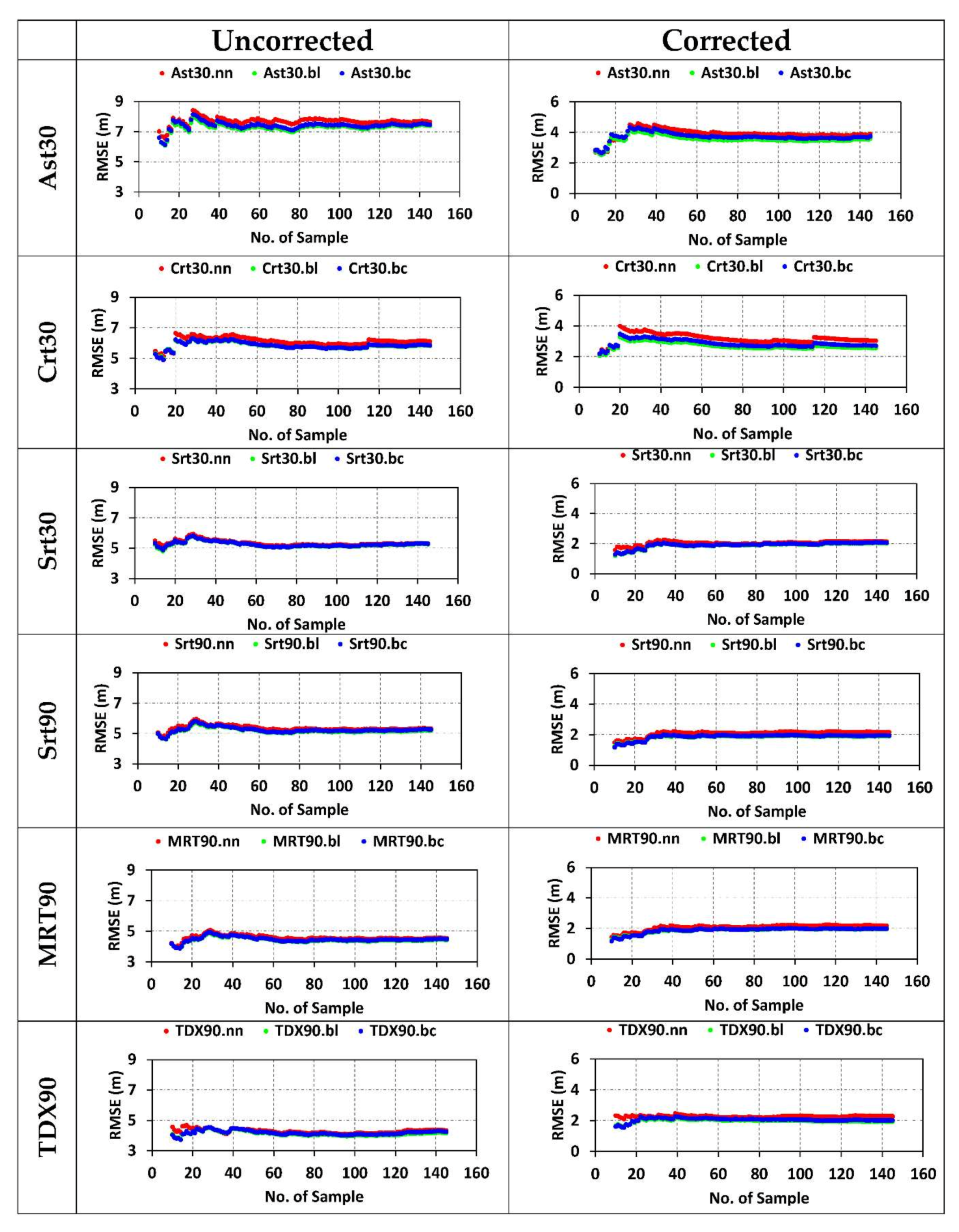
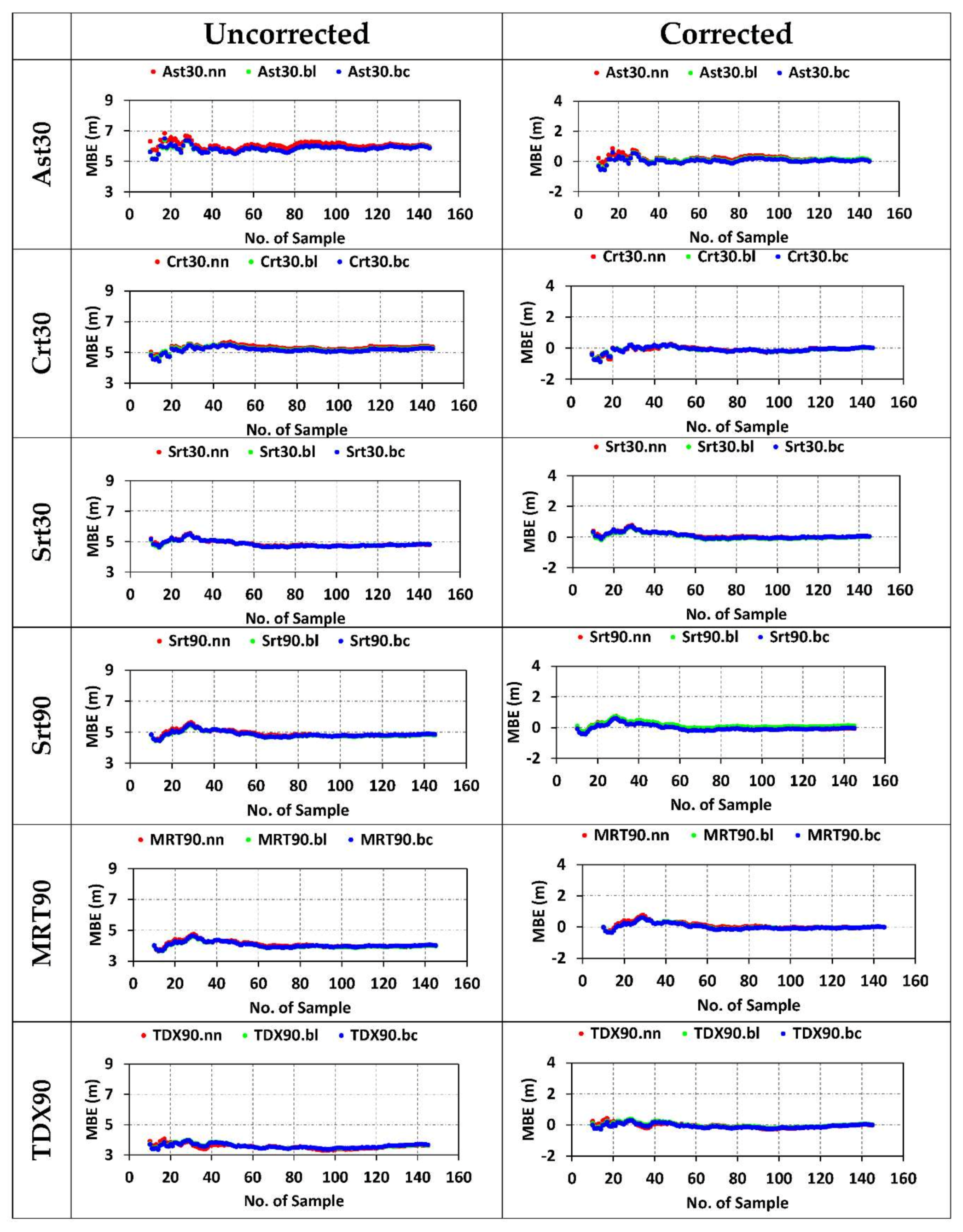
3.5. Optimum Number of GCPs
- In general, the variation in the calculated values of RMSE, MBE, SE, or RSD, with an increasing number of GCPs (randomly selected), exhibits a relatively sharper drop in the values up to approximately 40–60 GCPs and, thereafter, remains nearly invariable (for 60–145 no. of GCPs) for the corrected DEMs (Figure 5, Figure 6 and Figure 7 and Figure S7).
- As the changes in the values of RMSE, MBE, SE, and RSD are nearly invariable after 60 GCPs, it is noticeable that the optimum level of these errors are achievable with around 40–60 samples (minimum GCPs) for similar study areas.
4. Summary and Conclusions
- DGPS (dual-frequency with base-rover setup) provides much more robust estimates compared to single frequency MobileGPS in static mode. Thus, DGPS estimates at GCPs are recommended for use as a reference dataset for correction of DEMs.
- MobileGPS equipment may be considered as a relatively economically cheaper option for positioning purposes if the desired RMSE is within the range of approximately 5 m (for Northing), 10 m (for Easting), and 9 m (for Elevation).
- As the elevation values obtained from corrected DEMs are found to be consistent with respect to the reference dataset (DGPS) with a substantial reduction in error (RMSE, MBE, MAE), it is recommended that DEMs may be corrected using DGPS estimates over GCPs before use in any scientific studies.
- Correction to space-borne elevation datasets helps in reducing the bias by removing systematic error. The corrected DEMs show much lower values of RMSE, MBE, SE compared to the uncorrected DEMs.
- The significance test of changes brought by correction, as seen in the results of the statistical tests on the elevation and slope, corroborates the importance of correction of DEMs. For instance, the difference between the elevation values obtained from corrected DEMs and DGPS was found to be consistently insignificant (at 99% CL) for all cases (all DEMs and all interpolation methods). This implies that the DEMs and DGPS values are comparable after correction.
- The SRTM elevation data (Srt30) is one of the most preferred DEMs if correction is applied. However, without any correction, TanDEM-X (90 m) among the 90 m datasets and Srt30 or CartoDEM (30 m) among the 30 m datasets may be preferable over the Indian region due to the lower SE, RMSE, MBE, and MAE compared to other datasets.
- Srt30 is preferable as it has much finer spatial resolution (grid size) compared to Srt90, MRT90, and TDX90. The corrected Srt90, MRT90, and TDX90 (average of nn, bl, bc) show comparable RMSE (2.01 m, 2.05 m, and 2.09 m, respectively) and MBE is nearly zero when compared to that of Srt30 (RMSE of 2.08 m and MBE of 0.02 m). The slope values obtained from Srt30 are more realistic for ground flow modelling at a finer resolution compared to Srt90/MRT90/TDX90, where smoothening over a larger area may affect the ground flow model results.
- ASTER DEM (Ast30) shows relatively poor performance compared to SRTM, MERIT, TanDEM-X, and CartoDEM (Srt30, Srt90, MRT90, TDX90, and Crt30).
- Though the differences arising due to the interpolation methods can be considered to be negligible for all DEMs, the bilinear method (after correction) can be preferred as RMSE values are relatively lower compared to other methods. As the difference due to these methods is marginal in most cases, the choice of interpolation may depend upon the project objectives.
- For all DEMs, the slope values (average, minimum, and maximum) show only a marginal change in values before and after the correction of DEMs, implying that the slope values were largely unaffected while correcting for the elevation values (through the removal of systematic error).
- From the sensitivity of statistical measures (RMSE, MBE, SE, RSD) with the increasing number of GCPs, it was observed that the optimum number of GCPs required to achieve nearly stable values of (RMSE, MBE, SE, RSD) is around 40-60 in most cases when compared to 145 GCPs. Therefore, the minimum number of GCPs is recommended to be around 60 for study areas showing similar variability and range in the topography (a hard rock terrain that overall is flat-like with undulating and uneven surfaces).
Supplementary Materials
Author Contributions
Funding
Institutional Review Board Statement
Informed Consent Statement
Data Availability Statement
Acknowledgments
Conflicts of Interest
References
- Farr, T.G.; Rosen, P.A.; Caro, E.; Crippen, R.; Duren, R.; Hensley, S.; Kobrick, M.; Paller, M.; Rodriguez, E.; Roth, L.; et al. The Shuttle Radar Topography Mission. Rev. Geophys. 2007, 45, RG2004. [Google Scholar] [CrossRef]
- Hassan, A.A.A. Accuracy Assessment of Open Source Digital Elevation Models. J. Univ. Babylon Eng. Sci. 2018, 26, 23–33. [Google Scholar] [CrossRef]
- Das, A.; Lindenschmidt, K.-E. Evaluation of the Sensitivity of Hydraulic Model Parameters, Boundary Conditions and Digital Elevation Models on Ice-Jam Flood Delineation. Cold Reg. Sci. Technol. 2021, 183, 103218. [Google Scholar] [CrossRef]
- Wang, W.; Yang, X.; Yao, T. Evaluation of ASTER GDEM and SRTM and Their Suitability in Hydraulic Modelling of a Glacial Lake Outburst Flood in Southeast Tibet. Hydrol. Processes 2012, 26, 213–225. [Google Scholar] [CrossRef]
- Wise, S.M. Effect of Differing DEM Creation Methods on the Results from a Hydrological Model. Comput. Geosci. 2007, 33, 1351–1365. [Google Scholar] [CrossRef]
- Woodrow, K.; Lindsay, J.B.; Berg, A.A. Evaluating DEM Conditioning Techniques, Elevation Source Data, and Grid Resolution for Field-Scale Hydrological Parameter Extraction. J. Hydrol. 2016, 540, 1022–1029. [Google Scholar] [CrossRef]
- Hsu, Y.-C.; Prinsen, G.; Bouaziz, L.; Lin, Y.-J.; Dahm, R. An Investigation of DEM Resolution Influence on Flood Inundation Simulation. Procedia Eng. 2016, 154, 826–834. [Google Scholar] [CrossRef]
- Jafarzadegan, K.; Merwade, V. A DEM-Based Approach for Large-Scale Floodplain Mapping in Ungauged Watersheds. J. Hydrol. 2017, 550, 650–662. [Google Scholar] [CrossRef]
- Ganas, A.; Athanassiou, E. A Comparative Study on the Production of Satellite Orthoimagery for Geological Remote Sensing. Geocarto Int. 2000, 15, 53–62. [Google Scholar] [CrossRef]
- Li, J.; Zhao, Y.; Bates, P.; Neal, J.; Tooth, S.; Hawker, L.; Maffei, C. Digital Elevation Models for Topographic Characterisation and Flood Flow Modelling along Low-Gradient, Terminal Dryland Rivers: A Comparison of Spaceborne Datasets for the Río Colorado, Bolivia. J. Hydrol. 2020, 591, 125617. [Google Scholar] [CrossRef]
- Moudrỳ, V.; Lecours, V.; Gdulová, K.; Gábor, L.; Moudrá, L.; Kropáček, J.; Wild, J. On the Use of Global DEMs in Ecological Modelling and the Accuracy of New Bare-Earth DEMs. Ecol. Model. 2018, 383, 3–9. [Google Scholar] [CrossRef]
- Tsimi, C.; Ganas, A. Using the ASTER Global DEM to Derive Empirical Relationships among Triangular Facet Slope, Facet Height and Slip Rates along Active Normal Faults. Geomorphology 2015, 234, 171–181. [Google Scholar] [CrossRef]
- Yu, Y.; Kalashnikova, O.V.; Garay, M.J.; Lee, H.; Notaro, M. Identification and Characterization of Dust Source Regions across North Africa and the Middle East Using MISR Satellite Observations. Geophys. Res. Lett. 2018, 45, 6690–6701. [Google Scholar] [CrossRef]
- Feuerstein, S.; Schepanski, K. Identification of Dust Sources in a Saharan Dust Hot-Spot and Their Implementation in a Dust-Emission Model. Remote Sens. 2019, 11, 4. [Google Scholar] [CrossRef]
- Rayegani, B.; Barati, S.; Goshtasb, H.; Gachpaz, S.; Ramezani, J.; Sarkheil, H. Sand and Dust Storm Sources Identification: A Remote Sensing Approach. Ecol. Indic. 2020, 112, 106099. [Google Scholar] [CrossRef]
- Finlayson, D.P.; Montgomery, D.R.; Hallet, B. Spatial Coincidence of Rapid Inferred Erosion with Young Metamorphic Massifs in the Himalayas. Geology 2002, 30, 219–222. [Google Scholar] [CrossRef]
- Lavé, J.; Avouac, J.-P. Fluvial Incision and Tectonic Uplift across the Himalayas of Central Nepal. J. Geophys. Res. Solid Earth 2001, 106, 26561–26591. [Google Scholar] [CrossRef]
- Marinou, A.; Ganas, A.; Papazissi, K.; Paradissis, D. Demitris Paradissis Strain Patterns along the Kaparelli–Asopos Rift (Central Greece) from Campaign GPS Data. Ann. Geophys. 2015, 58, 6. [Google Scholar] [CrossRef]
- Rastogi, G.; Agrawal, R.; Prof, A. Bias Corrections of CartoDEM Using ICESat-GLAS Data in Hilly Regions. GIScience Remote Sens. 2015, 52, 571–585. [Google Scholar] [CrossRef]
- Elkhrachy, I. Vertical Accuracy Assessment for SRTM and ASTER Digital Elevation Models: A Case Study of Najran City, Saudi Arabia. Ain Shams Eng. J. 2018, 9, 1807–1817. [Google Scholar] [CrossRef]
- González-Moradas, M.D.R.; Viveen, W. Evaluation of ASTER GDEM2, SRTMv3.0, ALOS AW3D30 and TanDEM-X DEMs for the Peruvian Andes against Highly Accurate GNSS Ground Control Points and Geomorphological-Hydrological Metrics. Remote Sens. Environ. 2020, 237, 111509. [Google Scholar] [CrossRef]
- Jain, A.O.; Thaker, T.; Chaurasia, A.; Patel, P.; Singh, A.K. Vertical Accuracy Evaluation of SRTM-GL1, GDEM-V2, AW3D30 and CartoDEM-V3.1 of 30-m Resolution with Dual Frequency GNSS for Lower Tapi Basin India. Geocarto Int. 2018, 33, 1237–1256. [Google Scholar] [CrossRef]
- Mukherjee, S.; Joshi, P.K.; Mukherjee, S.; Ghosh, A.; Garg, R.D.; Mukhopadhyay, A. Evaluation of Vertical Accuracy of Open Source Digital Elevation Model (DEM). Int. J. Appl. Earth Obs. Geoinf. 2013, 21, 205–217. [Google Scholar] [CrossRef]
- Rawat, K.S.; Mishra, A.K.; Sehgal, V.K.; Ahmed, N.; Tripathi, V.K. Comparative Evaluation of Horizontal Accuracy of Elevations of Selected Ground Control Points from ASTER and SRTM DEM with Respect to CARTOSAT-1 DEM: A Case Study of Shahjahanpur District, Uttar Pradesh, India. Geocarto Int. 2013, 28, 439–452. [Google Scholar] [CrossRef]
- Zhang, K.; Gann, D.; Ross, M.; Robertson, Q.; Sarmiento, J.; Santana, S.; Rhome, J.; Fritz, C. Accuracy Assessment of ASTER, SRTM, ALOS, and TDX DEMs for Hispaniola and Implications for Mapping Vulnerability to Coastal Flooding. Remote Sens. Environ. 2019, 225, 290–306. [Google Scholar] [CrossRef]
- Gómez, M.F.; Lencinas, J.D.; Siebert, A.; Díaz, G.M. Accuracy Assessment of ASTER and SRTM DEMs: A Case Study in Andean Patagonia. GIScience Remote Sens. 2012, 49, 71–91. [Google Scholar] [CrossRef]
- Jalal, S.J.; Musa, T.A.; Ameen, T.H.; Din, A.H.M.; Aris, W.A.W.; Ebrahim, J.M. Optimizing the Global Digital Elevation Models (GDEMs) and Accuracy of Derived DEMs from GPS Points for Iraq’s Mountainous Areas. Geod. Geodyn. 2020, 11, 338–349. [Google Scholar] [CrossRef]
- Mukherjee, S. Accuracy of Cartosat-1 DEM and Its Derived Attribute at Multiple Scale Representation. J. Earth Syst. Sci. 2015, 124, 487–495. [Google Scholar] [CrossRef][Green Version]
- El-Quilish, M.; El-Ashquer, M.; Dawod, G.; El Fiky, G. Development and Accuracy Assessment of High-Resolution Digital Elevation Model Using GIS Approaches for the Nile Delta Region, Egypt. Am. J. Geogr. Inf. Syst. 2018, 7, 107–117. [Google Scholar]
- Soliman, A.; Han, L. Effects of Vertical Accuracy of Digital Elevation Model (DEM) Data on Automatic Lineaments Extraction from Shaded DEM. Adv. Space Res. 2019, 64, 603–622. [Google Scholar] [CrossRef]
- Patel, A.; Katiyar, S.K.; Prasad, V. Performances Evaluation of Different Open Source DEM Using Differential Global Positioning System (DGPS). Egypt. J. Remote Sens. Space Sci. 2016, 19, 7–16. [Google Scholar] [CrossRef]
- Muskett, R.R.; Lingle, C.S.; Sauber, J.M.; Post, A.S.; Tangborn, W.V.; Rabus, B.T.; Echelmeyer, K.A. Airborne and Spaceborne DEM- and Laser Altimetry-Derived Surface Elevation and Volume Changes of the Bering Glacier System, Alaska, USA, and Yukon, Canada, 1972–2006. J. Glaciol. 2009, 55, 316–326. [Google Scholar] [CrossRef]
- Rignot, E. Contribution of the Patagonia Icefields of South America to Sea Level Rise. Science 2003, 302, 434–437. [Google Scholar] [CrossRef]
- Sund, M.; Eiken, T.; Hagen, J.O.; Kääb, A. Svalbard Surge Dynamics Derived from Geometric Changes. Ann. Glaciol. 2009, 50, 50–60. [Google Scholar] [CrossRef]
- Chen, H.; Liang, Q.; Liu, Y.; Xie, S. Hydraulic Correction Method (HCM) to Enhance the Efficiency of SRTM DEM in Flood Modeling. J. Hydrol. 2018, 559, 56–70. [Google Scholar] [CrossRef]
- Giribabu, D.; Rao, S.S.; Murthy, Y.K. Improving Cartosat-1 DEM Accuracy Using Synthetic Stereo Pair and Triplet. ISPRS J. Photogramm. Remote Sens. 2013, 77, 31–43. [Google Scholar] [CrossRef]
- Jarihani, A.A.; Callow, J.N.; McVicar, T.R.; van Niel, T.G.; Larsen, J.R. Satellite-Derived Digital Elevation Model (DEM) Selection, Preparation and Correction for Hydrodynamic Modelling in Large, Low-Gradient and Data-Sparse Catchments. J. Hydrol. 2015, 524, 489–506. [Google Scholar] [CrossRef]
- Su, Y.; Guo, Q. A Practical Method for SRTM DEM Correction over Vegetated Mountain Areas. ISPRS J. Photogramm. Remote Sens. 2014, 87, 216–228. [Google Scholar] [CrossRef]
- Frey, H.; Paul, F. On the Suitability of the SRTM DEM and ASTER GDEM for the Compilation of Topographic Parameters in Glacier Inventories. Int. J. Appl. Earth Obs. Geoinf. 2012, 18, 480–490. [Google Scholar] [CrossRef]
- Ahmed, N.; Mahtab, A.; Agrawal, R.; Jayaprasad, P.; Pathan, S.K.; Ajai; Singh, D.K.; Singh, A.K. Extraction and Validation of Cartosat-1 DEM. J. Indian Soc. Remote Sens. 2007, 35, 121–127. [Google Scholar] [CrossRef]
- Shen, J.; Tan, F. Effects of DEM Resolution and Resampling Technique on Building Treatment for Urban Inundation Modeling: A Case Study for the 2016 Flooding of the HUST Campus in Wuhan. Nat. Hazards 2020, 104, 927–957. [Google Scholar] [CrossRef]
- Tan, M.L.; Ficklin, D.L.; Dixon, B.; Ibrahim, A.L.; Yusop, Z.; Chaplot, V. Impacts of DEM Resolution, Source, and Resampling Technique on SWAT-Simulated Streamflow. Appl. Geogr. 2015, 63, 357–368. [Google Scholar] [CrossRef]
- Tan, M.L.; Ramli, H.P.; Tam, T.H. Effect of DEM Resolution, Source, Resampling Technique and Area Threshold on SWAT Outputs. Water Resour. Manag. 2018, 32, 4591–4606. [Google Scholar] [CrossRef]
- Arun, P.V. A Comparative Analysis of Different DEM Interpolation Methods. Egypt. J. Remote Sens. Space Sci. 2013, 16, 133–139. [Google Scholar] [CrossRef]
- Zimmerman, D.; Pavlik, C.; Ruggles, A.; Armstrong, M.P. An Experimental Comparison of Ordinary and Universal Kriging and Inverse Distance Weighting. Math. Geol. 1999, 31, 375–390. [Google Scholar] [CrossRef]
- Saksena, S.; Merwade, V. Incorporating the Effect of DEM Resolution and Accuracy for Improved Flood Inundation Mapping. J. Hydrol. 2015, 530, 180–194. [Google Scholar] [CrossRef]
- Szot, T.; Specht, C.; Specht, M.; Dabrowski, P.S. Comparative Analysis of Positioning Accuracy of Samsung Galaxy Smartphones in Stationary Measurements. PLoS ONE 2019, 14, e0215562. [Google Scholar] [CrossRef]
- Aguilar, F.J.; Agüera, F.; Aguilar, M.A. A Theoretical Approach to Modeling the Accuracy Assessment of Digital Elevation Models. Photogramm. Eng. Remote Sens. 2007, 73, 1367–1379. [Google Scholar] [CrossRef][Green Version]
- Muralikrishnan, S.; Reddy, S.; Narender, B.; Pillai, A. Evaluation of Indian National DEM from Cartosat-1 Data Summary Report (Ver. 1); NRSC-AS&DM-DP&VASDSEP11-TR 286. 2011. Available online: https://bhuvan-app3.nrsc.gov.in/data/download/tools/document/CartoDEMReadme_v1_u1_23082011.pdf (accessed on 16 November 2021).
- Mouratidis, A.; Briole, P.; Katsambalos, K. SRTM 3″ DEM (Versions 1, 2, 3, 4) Validation by Means of Extensive Kinematic GPS Measurements: A Case Study from North Greece. Int. J. Remote Sens. 2010, 31, 6205–6222. [Google Scholar] [CrossRef]
- Thomas, J.; Joseph, S.; Thrivikramji, K.P.; Arunkumar, K.S. Sensitivity of Digital Elevation Models: The Scenario from Two Tropical Mountain River Basins of the Western Ghats, India. Geosci. Front. 2014, 5, 893–909. [Google Scholar] [CrossRef]
- Rawat, K.S.; Singh, S.K.; Singh, M.I.; Garg, B. Comparative Evaluation of Vertical Accuracy of Elevated Points with Ground Control Points from ASTERDEM and SRTMDEM with Respect to CARTOSAT-1DEM. Remote Sens. Appl. Soc. Environ. 2019, 13, 289–297. [Google Scholar] [CrossRef]
- NASA/METI/AIST/Japan Spacesystems and U.S./Japan ASTER Science Team. ASTER Global Digital Elevation Model V003. 2019. Available online: https://lpdaac.usgs.gov/documents/434/ASTGTM_User_Guide_V3.pdf (accessed on 16 November 2021).
- ASTER Global. ASTER Global Digital Elevation Map Announcement. Available online: http://asterweb.jpl.nasa.gov/gdem (accessed on 16 November 2021).
- Tachikawa, T.; Kaku, M.; Iwasaki, A.; Gesch, D.B.; Oimoen, M.J.; Zhang, Z.; Danielson, J.J.; Krieger, T.; Curtis, B.; Haase, J. ASTER Global Digital Elevation Model Version 2-Summary of Validation Results; NASA, 2011. Available online: https://lpdaac.usgs.gov/documents/220/Summary_GDEM2_validation_report_final.pdf (accessed on 16 November 2021).
- Chen, C.; Yang, S.; Li, Y. Accuracy Assessment and Correction of SRTM DEM Using ICESat/GLAS Data under Data Coregistration. Remote Sens. 2020, 12, 3435. [Google Scholar] [CrossRef]
- Van Zyl, J.J. The Shuttle Radar Topography Mission (SRTM): A Breakthrough in Remote Sensing of Topography. Acta Astronaut. 2001, 48, 559–565. [Google Scholar] [CrossRef]
- Earth Resources Observation And Science Center. Shuttle Radar Topography Mission (SRTM) 1 Arc-Second Global. 2017. Available online: https://cmr.earthdata.nasa.gov/search/concepts/C1220567890-USGS_LTA.html (accessed on 27 November 2019).
- Sun, G.; Ranson, K.J.; Kharuk, V.I.; Kovacs, K. Validation of Surface Height from Shuttle Radar Topography Mission Using Shuttle Laser Altimeter. Remote Sens. Environ. 2003, 88, 401–411. [Google Scholar] [CrossRef]
- Gorokhovich, Y.; Voustianiouk, A. Accuracy Assessment of the Processed SRTM-Based Elevation Data by CGIAR Using Field Data from USA and Thailand and Its Relation to the Terrain Characteristics. Remote Sens. Environ. 2006, 104, 409–415. [Google Scholar] [CrossRef]
- Van Niel, T.G.; McVicar, T.R.; Li, L.; Gallant, J.C.; Yang, Q. The Impact of Misregistration on SRTM and DEM Image Differences. Remote Sens. Environ. 2008, 112, 2430–2442. [Google Scholar] [CrossRef]
- NASA SRTM V3. NASA Shuttle Radar Topography Mission (SRTM) Version 3.0 Global 1 Arc Second Data Released over Asia and Australia|Earthdata. Available online: https://earthdata.nasa.gov/learn/articles/nasa-shuttle-radar-topography-mission-srtm-version-3-0-global-1-arc-second-data-released-over-asia-and-australia/ (accessed on 5 December 2021).
- Rodríguez, E.; Morris, C.S.; Belz, J.E. A Global Assessment of the SRTM Performance. Photogramm. Eng. Remote Sens. 2006, 72, 249–260. [Google Scholar] [CrossRef]
- Muralikrishnan, S.; Pillai, A.; Narender, B.; Reddy, S.; Venkataraman, V.R.; Dadhwal, V.K. Validation of Indian National DEM from Cartosat-1 Data. J. Indian Soc. Remote Sens. 2013, 41, 1–13. [Google Scholar] [CrossRef]
- Muralikrishnan, S.; Kumar, A.S.; Manjunath, A.; Rao, K. Geometric Quality Assessment of Cartosat-1 Data Products. Available online: https://www.isprs.org/proceedings/XXXVI/part4/WG-IV-9-20.pdf (accessed on 27 January 2019).
- Muralikrishnan, S.; Narender, B.; Reddy, S.; Pillai, A. Evaluation of Indian National from Cartosat-1 Data. Indian Space Res. Organ.-NRSC 2014, 2, 1–55. Available online: https://bhuvan-app3.nrsc.gov.in/data/download/tools/document/Evaluation%20of%20Indian%20National%20DEM%20Version_2%20using%20Cartosat-1%20data%20Dec%202014.pdf (accessed on 16 November 2021).
- Liu, Y.; Bates, P.D.; Neal, J.C.; Yamazaki, D. Bare-Earth DEM Generation in Urban Areas for Flood Inundation Simulation Using Global Digital Elevation Models. Water Resour. Res. 2021, 57, e2020WR028516. [Google Scholar] [CrossRef]
- Yamazaki, D.; Ikeshima, D.; Tawatari, R.; Yamaguchi, T.; O’Loughlin, F.; Neal, J.C.; Sampson, C.C.; Kanae, S.; Bates, P.D. A High-Accuracy Map of Global Terrain Elevations: Accurate Global Terrain Elevation Map. Geophys. Res. Lett. 2017, 44, 5844–5853. [Google Scholar] [CrossRef]
- Krieger, G.; Moreira, A.; Fiedler, H.; Hajnsek, I.; Werner, M.; Younis, M.; Zink, M. TanDEM-X: A Satellite Formation for High-Resolution SAR Interferometry. IEEE Trans. Geosci. Remote Sens. 2007, 45, 3317–3341. [Google Scholar] [CrossRef]
- Rizzoli, P.; Martone, M.; Gonzalez, C.; Wecklich, C.; Borla Tridon, D.; Bräutigam, B.; Bachmann, M.; Schulze, D.; Fritz, T.; Huber, M.; et al. Generation and Performance Assessment of the Global TanDEM-X Digital Elevation Model. ISPRS J. Photogramm. Remote Sens. 2017, 132, 119–139. [Google Scholar] [CrossRef]
- Zink, M.; Bachmann, M.; Brautigam, B.; Fritz, T.; Hajnsek, I.; Moreira, A.; Wessel, B.; Krieger, G. TanDEM-X: The New Global DEM Takes Shape. IEEE Geosci. Remote Sens. Mag. 2014, 2, 8–23. [Google Scholar] [CrossRef]
- Zink, M.; Moreira, A.; Hajnsek, I.; Rizzoli, P.; Bachmann, M.; Kahle, R.; Fritz, T.; Huber, M.; Krieger, G.; Lachaise, M.; et al. TanDEM-X: 10 Years of Formation Flying Bistatic SAR Interferometry. IEEE J. Sel. Top. Appl. Earth Obs. Remote Sens. 2021, 14, 3546–3565. [Google Scholar] [CrossRef]
- Han, H.; Zeng, Q.; Jiao, J. Quality Assessment of TanDEM-X DEMs, SRTM and ASTER GDEM on Selected Chinese Sites. Remote Sens. 2021, 13, 1304. [Google Scholar] [CrossRef]
- Hawker, L.; Neal, J.; Bates, P. Accuracy Assessment of the TanDEM-X 90 Digital Elevation Model for Selected Floodplain Sites. Remote Sens. Environ. 2019, 232, 111319. [Google Scholar] [CrossRef]
- Wessel, B. TanDEM-X Ground Segment DEM Products Specification Document; Public Document TD-GS-PS-0021. 2016; Volume 46. Available online: https://elib.dlr.de/108014/1/TD-GS-PS-0021_DEM-Product-Specification_v3.1.pdf (accessed on 16 November 2021).
- Wessel, B.; Huber, M.; Wohlfart, C.; Marschalk, U.; Kosmann, D.; Roth, A. Accuracy Assessment of the Global TanDEM-X Digital Elevation Model with GPS Data. ISPRS J. Photogramm. Remote Sens. 2018, 139, 171–182. [Google Scholar] [CrossRef]
- Gonzalez, C.; Rizzoli, P. Landcover-Dependent Assessment of the Relative Height Accuracy in TanDEM-X DEM Products. IEEE Geosci. Remote Sens. Lett. 2018, 15, 1892–1896. [Google Scholar] [CrossRef]
- Briole, P.; Bufferal, S.; Dimitrov, D.; Elias, P.; Journeau, C.; Avallone, A.; Kamberos, K.; Capderou, M.; Nercessian, A. Using Kinematic GNSS Data to Assess the Accuracy and Precision of the TanDEM-X DEM Resampled at 1-m Resolution Over the Western Corinth Gulf, Greece. IEEE J. Sel. Top. Appl. Earth Obs. Remote Sens. 2021, 14, 3016–3025. [Google Scholar] [CrossRef]
- Bhardwaj, A. Assessment of Vertical Accuracy for TanDEM-X 90 m DEMs in Plain, Moderate, and Rugged Terrain. Proceedings 2019, 24, 8. [Google Scholar] [CrossRef]
- Uuemaa, E.; Ahi, S.; Montibeller, B.; Muru, M.; Kmoch, A. Vertical Accuracy of Freely Available Global Digital Elevation Models (ASTER, AW3D30, MERIT, TanDEM-X, SRTM, and NASADEM). Remote Sens. 2020, 12, 3482. [Google Scholar] [CrossRef]
- El-Rabbany, A. Artech House mobile communications series. In Introduction to GPS: The Global Positioning System; Artech House: Boston, MA, USA, 2002; ISBN 978-1-58053-183-2. [Google Scholar]
- Drira, A. GPS Navigation for Outdoor and Indoor Environments. University of Tennessee, Knoxville; 2006. Available online: https://www.imaging.utk.edu/publications/papers/dissertation/Anis_Pilot.pdf (accessed on 27 January 2019).
- Horecny, V. Can We Trust A-GPS Technology to Deliver Accurate Location on a Smartphone Device? 2016. Available online: https://www.semanticscholar.org/paper/Can-we-trust-A-GPS-technology-to-deliver-accurate-a-Horecny/eee167c4fcde97b609a499c403b7e1d3cd4de7e2 (accessed on 27 January 2019).
- Gdal_translate—GDAL Documentation. Available online: https://gdal.org/programs/gdal_translate.html#gdal-translate (accessed on 23 December 2021).
- GeographicLib—Browse/Geoids-Distrib at SourceForge.Net. Available online: https://sourceforge.net/projects/geographiclib/files/geoids-distrib/ (accessed on 23 December 2021).
- Kaplan, E.D.; Hegarty, C.J. (Eds.) Understanding GPS: Principles and Applications, 2nd ed.; Artech House Mobile Communications Series; Artech House: Boston, MA, USA, 2006; ISBN 978-1-58053-894-7. [Google Scholar]
- Geoid Height Calculator|Software|UNAVCO. Available online: https://www.unavco.org/software/geodetic-utilities/geoid-height-calculator/geoid-height-calculator.html (accessed on 23 December 2021).
- Cakir, L.; Konakoglu, B. The Impact of Data Normalization on 2D Coordinate Transformation Using GRNN. Geod. Vestn. 2019, 63, 541–553. [Google Scholar] [CrossRef]
- Ruiz, G.; Bandera, C. Validation of Calibrated Energy Models: Common Errors. Energies 2017, 10, 1587. [Google Scholar] [CrossRef]
- National Bureau of Standards; NBS Special Publication; ASTM Special Technical Publication; U.S. Government Printing Office. 1969. Available online: https://books.google.com/books/download/NBS_Special_Publication.pdf?id=mp3kUzm76RYC&output=pdf (accessed on 27 January 2019).
- Ma, Y.; Liu, H.; Jiang, B.; Meng, L.; Guan, H.; Xu, M.; Cui, Y.; Kong, F.; Yin, Y.; Wang, M. An Innovative Approach for Improving the Accuracy of Digital Elevation Models for Cultivated Land. Remote Sens. 2020, 12, 3401. [Google Scholar] [CrossRef]
- DeWitt, J.D.; Warner, T.A.; Conley, J.F. Comparison of DEMS Derived from USGS DLG, SRTM, a Statewide Photogrammetry Program, ASTER GDEM and LiDAR: Implications for Change Detection. GIScience Remote Sens. 2015, 52, 179–197. [Google Scholar] [CrossRef]
- Bhardwaj, A. Evaluation of DEM, and Orthoimage Generated from Cartosat-1 with Its Potential for Feature Extraction and Visualization. Am. J. Remote Sens. 2013, 1, 1–6. [Google Scholar] [CrossRef][Green Version]
- Santillan, J.R.; Makinano-Santillan, M. Vertical accuracy assessment of 30-m resolution alos, aster, and srtm global dems over northeastern mindanao, philippines. Int. Arch. Photogramm. Remote Sens. Spat. Inf. Sci. 2016, XLI-B4, 149–156. [Google Scholar] [CrossRef]
- Suwandana, E.; Kawamura, K.; Sakuno, Y.; Kustiyanto, E.; Raharjo, B. Evaluation of ASTER GDEM2 in Comparison with GDEM1, SRTM DEM and Topographic-Map-Derived DEM Using Inundation Area Analysis and RTK-DGPS Data. Remote Sens. 2012, 4, 2419–2431. [Google Scholar] [CrossRef]
- Talchabhadel, R.; Nakagawa, H.; Kawaike, K.; Yamanoi, K.; Thapa, B.R. Assessment of Vertical Accuracy of Open Source 30m Resolution Space-Borne Digital Elevation Models. Geomat. Nat. Hazards Risk 2021, 12, 939–960. [Google Scholar] [CrossRef]
- Grohmann, C.H. Evaluation of TanDEM-X DEMs on Selected Brazilian Sites: Comparison with SRTM, ASTER GDEM and ALOS AW3D30. Remote Sens. Environ. 2018, 212, 121–133. [Google Scholar] [CrossRef]
- Tridon, D.B.; Bachmann, M.; Schulze, D.; Míguez, C.O.; Polimeni, M.D.; Martone, M.; Böer, J.; Zink, M. TanDEM-X: DEM Acquisition in the Third Year Era. Int. J. Space Sci. Eng. 2013, 1, 367. [Google Scholar] [CrossRef]
- Radhika, V.N.; Kartikeyan, B.; Krishna, B.G.; Chowdhury, S.; Srivastava, P.K. Robust Stereo Image Matching for Spaceborne Imagery. IEEE Trans. Geosci. Remote Sens. 2007, 45, 2993–3000. [Google Scholar] [CrossRef]


| Sl. | Author | Study Area | No. of GCPs. Land Cover Type | DEM Used and Corresponding RMSE/Bias/Other Statistics | ||||
|---|---|---|---|---|---|---|---|---|
| 1. | [22] | Lower Tapi Basin, India, 3837 km2 | GCPs = 117. Topography comprising narrow valley, hilly terrain, gently sloping ground, agricultural fields and coastal regions | RMSE values of DEM elevation for:
| ||||
| 2. | [29] | Nile, delta Region, 23,235 km2 | GCPs = 200. Delta region | RMSE values of DEM elevation for:
| ||||
| 3. | [20] | Najran City, Saudi Arabia, 900 km2 | GCPs = 50 (with outlier) 49 for ASTER and 48 for SRTM30 after removing outlier. Mountainous area with high elevation differences | RMSE values with and without outlier:
| ||||
| 4. | [31] | MANITB, M.P., India | GCPs = 830. Uneven topography with small hills | RMSE values of DEM elevation without applying any interpolation for:
| ||||
| 5. | [47] | Comparison of Samsung smartphones | Samsung Galaxy series Y, S3 Mini, S4, S5, S6 and S7 | Two newest generations smartphones, S6 and S7 obtained lower vertical accuracies than their predecessors with RMSE for:
| ||||
| 6. | [23] | Western Shiwalik, Himalaya, India | GCPs = 11. Topography dominated by hills, valleys, steep slopes and rivers | RMSE values of DEM elevation for:
| ||||
| 7. | [26] | Andean Patagonia, Argentina, 540 km2 | GCPs = 78 Rugged Topography | RMSE values of DEM elevation for:
| ||||
| 8. | [28] | Shiwalik Himalaya, India | GCPs = 11. Rugged terrain with steep slopes, ridges, undulations with flat topography in southern part | RMSE values for Cartosat-1 DEM: 3.14–7.24 m, varying with grid spacing from 10–150 m | ||||
| 9. | [19] | Chandra and Bhaga Basin, Himalayan Region, India | GCPs = 2835 (Chandra). GCPs = 2160 (Bhaga). Basin | Bias of elevation data for:
| ||||
| 10. | [38] | SNAMP and CZO, USA | GCPs = − Coastal Vegetated Mountainous Areas | Correction applied to SRTM DEM RMSE values fof DEM elevation, prior to and after correction, for SRTM DEM are:
| ||||
| 11. | [36] | Himalayan Region, India | GCPs = 6. Rugged and hilly topography | RMSE values for Cartosat-1 DEM:
| ||||
| 12. | [24] | Shahjahanpur district, UP, India | GCPs = 20 Plains of Ganga interrupted by valleys and numerous streams | Horizontal accuracy of ASTER GDEM1and SRTM90 DEM with respect to Cartosat-1 is evaluated. RMSE for horizontal accuracy are:
| ||||
| 13. | [49] | Jagathsinghpur, Orissa (flat); Dharmsala, Himachal Pradesh (hilly); Alwar, Rajasthan (mixed) | GCPs = 15 (Jagathsinghpur), 8 (Dharmsala), 59 (ICP over Alwar). Flat, hilly and mixed type | RMSE for CatoDEM30 elevation data at
| ||||
| 14. | [50] | Thessaloniki, North Greece | ICESat reference Points = 10,792. Varying topography: flat to mountainous. | Standard deviation of absolute elevation error for:
| ||||
| 15. | [51] | MRB: Muthirapuzha River Basin (271.75 km2). PRB: Pambar River Basin (288.53 km2) | GCPs = 28. Topography is dominated by hills and plateau | RMSE values for various DEMs | ||||
| Relief (m/km2) | ||||||||
| DEMs | Area | <200 | 200–400 | >400 | ||||
| TOPO | MRB | 11.07 | 9.54 | 8.11 | ||||
| PRB | 6.15 | 10.34 | 10.36 | |||||
| ASTER | MRB | 21.83 | 31.75 | 42.08 | ||||
| PRB | 9.16 | 19.26 | 33.12 | |||||
| SRTM | MRB | 10.46 | 22.51 | 29.55 | ||||
| PRB | 10.86 | 15.88 | 27.68 | |||||
| GMTED | MRB | 36.54 | 50.99 | 86.75 | ||||
| PRB | 33.78 | 40.49 | 62.09 | |||||
| 16. | [52] | Roja Village, UP, India,4575 km2 | GCPs = 20 Upland plains of Ganga valley, predominated by valleys, streams, and water sources | RMSE values for DEM elevation, taking elevation values of CARTOSAT-1 DEM as reference, for:
| ||||
| 17. | [21] | Peru | GCPs = 139 Flat, Arid Coast, Semi-dry Andes, Amazon rainforest | RMSE values of DEM elevation for:
| ||||
| 18. | [10] | Rio Colorado, Bolivia | GCPs = 1290 Basin type located at ocean-continent convergent margin | RMSE values of DEM elevation for:
| ||||
| 19. | [27] | Iraq | GCPs = 12 Mountainous | RMSE values for:
| ||||
| 20. | [25] | Hispaniola, USA, 75,000 km2 | GCPs = 2287 Topography dominated by Mountains and valleys, coastal areas | RMSE values of DEM elevation for:
| ||||
| 21. | [30] | Baoji city, China, 2500 km2 | GCPs = - Combination of flat, hilly and mountainous areas | RMSE values of DEM elevation for:
| ||||
| DEM Details | ASTER (30 m) | CARTOSAT-1 (30 m) | SRTM (30 m) | SRTM (90 m) | MERIT DEM (90 m) | TanDEM-X (90 m) |
|---|---|---|---|---|---|---|
| Release Year | 2019 | 2005 | 2015 | 2008 | 2017 | 2018 |
| Product Format | GEOTIFF | GEOTIFF | GEOTIFF | GEOTIFF | GEOTIFF | GEOTIFF |
| Co-ordinate System | GCS_WGS_1984 | GCS_WGS_1984 | GCS_WGS_1984 | GCS_WGS_1984 | GCS_WGS_1984 | GCS_WGS_1984 |
| Sensor | ASTER | Pan (2.5 m) | SIR-C X-SAR | SIR-C X-SAR | SIR-C X-SAR | SAR-X Band |
| Satellite | Terra | Cartosat-1 | Space Shuttle Endeavour | Space Shuttle Endeavour | Space Shuttle Endeavour | TerraSAR-X and TanDEM-X |
| Resolution | 30 m | 30 m | 30 m | 90 m | 90 m | 90 m |
| Projection | Geographic (Lat., Long.) | Geographic (Lat., Long.) | Geographic (Lat., Long.) | Geographic (Lat., Long.) | Geographic (Lat., Long.) | Geographic (Lat., Long.) |
| Datum | WGS_1984 (H) EGM96 (V) | WGS_1984 (H) WGS_1984 (V) | WGS_1984 (H) EGM96 (V) | WGS_1984 (H) EGM96 (V) | WGS_1984 (H) EGM96 (V) | WGS_1984 (H) WGS_1984 (V) |
| Version | V3 | V3 R1 | V3 | V4.1 | V1 | V1 |
| Data Sources | https://earthexplorer.usgs.gov/ | http://bhuvan.nrsc.gov.in | https://earthexplorer.usgs.gov/ | http://srtm.csi.cgiar.org/ | http://hydro.iis.u-tokyo.ac.jp/~yamadai/MERIT_DEM/ | https://download.geoservice.dlr.de/TDM90/ |
| Last Accessed | 16 November 2021 | 27 January 2019 | 27 January 2019 | 27 January 2019 | 16 November 2021 | 16 November 2021 |
| Elevation (Z) | Easting (E) | Northing (N) | ||
|---|---|---|---|---|
| Avg. (in m) | DGPS | 244.41 | - | - |
| MobileGPS | 243.09 | - | - | |
| Max. (in m) | DGPS | 257.63 | - | - |
| MobileGPS | 275.12 | - | - | |
| Min. (in m) | DGPS | 230.22 | - | - |
| MobileGPS | 221.11 | - | - | |
| SD (in m) | DGPS | 5.85 | - | - |
| MobileGPS | 9.54 | - | - | |
| RSD (in %) | DGPS | 2.39 | - | - |
| MobileGPS | 3.92 | - | - | |
| SE (in m) | DGPS | 0.49 | - | - |
| MobileGPS | 0.79 | - | - | |
| RMSE (in m) | MobileGPS–DGPS | 8.93 | 10.10 | 5.02 |
| RMSE(in %) | MobileGPS–DGPS | 3.68 | - | - |
| MBE (in m) | MobileGPS–DGPS | −1.32 | 0.49 | 1.43 |
| MBE (in %) | MobileGPS–DGPS | −0.52 | - | - |
| MAE (in m) | MobileGPS -DGPS | 6.21 | 4.59 | 3.56 |
| Mean (Z) (in m) | SD (in m) | SE (in m) | RMSE (in m) | RMSE% | MBE (in m) | MBE% | MAE (in m) | RSD % | |||||||||||
|---|---|---|---|---|---|---|---|---|---|---|---|---|---|---|---|---|---|---|---|
| u | c | u | c | u | c | u | c | u | c | u | c | u | c | u | c | u | c | ||
| Ast30 | nn | 250.37 | 244.46 | 8.41 | 7.04 | 0.70 | 0.58 | 7.65 | 3.91 | 3.12 | 1.60 | 5.96 | 0.05 | 2.43 | 0.02 | 6.35 | 3.11 | 3.37 | 2.89 |
| bl | 250.29 | 244.51 | 8.25 | 6.88 | 0.68 | 0.57 | 7.39 | 3.61 | 3.01 | 1.48 | 5.89 | 0.10 | 2.40 | 0.04 | 6.18 | 2.86 | 3.30 | 2.82 | |
| bc | 250.28 | 244.42 | 8.32 | 6.95 | 0.69 | 0.58 | 7.47 | 3.75 | 3.04 | 1.53 | 5.87 | 0.01 | 2.39 | 0.01 | 6.21 | 2.97 | 3.33 | 2.85 | |
| Crt30 | nn | 249.78 | 244.40 | 6.20 | 6.60 | 0.51 | 0.55 | 6.10 | 3.04 | 2.51 | 1.26 | 5.37 | 0.00 | 2.20 | 0.00 | 5.37 | 2.22 | 2.49 | 2.71 |
| bl | 249.69 | 244.40 | 6.04 | 6.39 | 0.50 | 0.53 | 5.83 | 2.58 | 2.40 | 1.07 | 5.29 | −0.01 | 2.17 | 0.00 | 5.29 | 1.97 | 2.43 | 2.62 | |
| bc | 249.65 | 244.42 | 6.10 | 6.46 | 0.51 | 0.54 | 5.85 | 2.72 | 2.41 | 1.13 | 5.25 | 0.01 | 2.15 | 0.01 | 5.25 | 2.06 | 2.45 | 2.65 | |
| Srt30 | nn | 249.21 | 244.43 | 6.49 | 6.23 | 0.54 | 0.52 | 5.31 | 2.14 | 2.17 | 0.88 | 4.81 | 0.02 | 1.97 | 0.01 | 4.84 | 1.71 | 2.61 | 2.56 |
| bl | 249.23 | 244.41 | 6.39 | 6.20 | 0.53 | 0.51 | 5.27 | 2.04 | 2.16 | 0.84 | 4.83 | 0.01 | 1.97 | 0.00 | 4.85 | 1.64 | 2.57 | 2.54 | |
| bc | 249.24 | 244.45 | 6.43 | 6.18 | 0.53 | 0.51 | 5.29 | 2.07 | 2.17 | 0.86 | 4.83 | 0.05 | 1.98 | 0.02 | 4.86 | 1.65 | 2.59 | 2.53 | |
| Srt90 | nn | 249.23 | 244.34 | 6.40 | 6.24 | 0.53 | 0.52 | 5.31 | 2.16 | 2.17 | 0.89 | 4.82 | −0.06 | 1.97 | −0.03 | 4.84 | 1.79 | 2.58 | 2.56 |
| bl | 249.23 | 244.51 | 6.19 | 6.16 | 0.51 | 0.51 | 5.19 | 1.91 | 2.13 | 0.79 | 4.82 | 0.10 | 1.97 | 0.04 | 4.82 | 1.59 | 2.49 | 2.53 | |
| bc | 249.27 | 244.37 | 6.31 | 6.16 | 0.52 | 0.51 | 5.26 | 1.94 | 2.15 | 0.80 | 4.87 | −0.04 | 1.99 | −0.02 | 4.87 | 1.62 | 2.54 | 2.53 | |
| MRT90 | nn | 248.40 | 244.40 | 6.19 | 6.24 | 0.51 | 0.52 | 4.54 | 2.18 | 1.86 | 0.90 | 3.99 | −0.01 | 1.63 | 0.00 | 4.03 | 1.81 | 2.50 | 2.56 |
| bl | 248.40 | 244.40 | 6.01 | 6.17 | 0.50 | 0.51 | 4.43 | 1.97 | 1.82 | 0.82 | 3.99 | 0.00 | 1.64 | 0.00 | 3.99 | 1.67 | 2.43 | 2.54 | |
| bc | 248.44 | 244.40 | 6.12 | 6.18 | 0.51 | 0.51 | 4.49 | 1.99 | 1.84 | 0.82 | 4.03 | 0.00 | 1.65 | 0.00 | 4.04 | 1.68 | 2.47 | 2.54 | |
| TDX90 | nn | 248.03 | 244.39 | 6.58 | 6.28 | 0.55 | 0.52 | 4.35 | 2.28 | 1.78 | 0.94 | 3.62 | −0.01 | 1.48 | −0.01 | 3.71 | 1.85 | 2.66 | 2.58 |
| bl | 248.06 | 244.43 | 6.34 | 6.17 | 0.53 | 0.51 | 4.17 | 1.95 | 1.71 | 0.81 | 3.65 | 0.02 | 1.49 | 0.01 | 3.66 | 1.64 | 2.56 | 2.53 | |
| bc | 248.09 | 244.41 | 6.49 | 6.19 | 0.54 | 0.51 | 4.27 | 2.03 | 1.75 | 0.84 | 3.69 | 0.00 | 1.51 | 0.00 | 3.70 | 1.70 | 2.62 | 2.54 | |
| Avg. of nn, bl & bc | Ast30 | 250.31 | 244.46 | 8.33 | 6.96 | 0.69 | 0.58 | 7.51 | 3.75 | 3.06 | 1.54 | 5.91 | 0.05 | 2.41 | 0.02 | 6.25 | 2.98 | 3.33 | 2.85 |
| Crt30 | 249.71 | 244.41 | 6.11 | 6.48 | 0.51 | 0.54 | 5.93 | 2.78 | 2.44 | 1.15 | 5.30 | 0.00 | 2.17 | 0.00 | 5.30 | 2.08 | 2.46 | 2.66 | |
| Srt30 | 249.23 | 244.43 | 6.44 | 6.20 | 0.53 | 0.51 | 5.29 | 2.08 | 2.17 | 0.86 | 4.82 | 0.02 | 1.97 | 0.01 | 4.85 | 1.67 | 2.59 | 2.54 | |
| Srt90 | 249.24 | 244.41 | 6.30 | 6.19 | 0.52 | 0.51 | 5.25 | 2.01 | 2.15 | 0.83 | 4.84 | 0.00 | 1.98 | 0.00 | 4.84 | 1.67 | 2.54 | 2.54 | |
| MRT90 | 248.41 | 244.40 | 6.11 | 6.20 | 0.51 | 0.51 | 4.49 | 2.05 | 1.84 | 0.85 | 4.01 | 0.00 | 1.64 | 0.00 | 4.02 | 1.72 | 2.47 | 2.55 | |
| TDX90 | 248.06 | 244.41 | 6.47 | 6.21 | 0.54 | 0.52 | 4.26 | 2.09 | 1.74 | 0.86 | 3.65 | 0.00 | 1.49 | 0.00 | 3.69 | 1.73 | 2.62 | 2.55 | |
| Aster30 |
|---|
| Ast30.nn.overDGPS = −41.76 + (1.195 × DGPS) |
| Ast30.bl.overDGPS = −42.87 + (1.199 × DGPS) |
| Ast30.bc.overDGPS = −42.05 + (1.196 × DGPS) |
| CRT30 |
| Crt30.nn.overDGPS = 20.21 + (0.9393 × DGPS) |
| Crt30.bl.overDGPS = 18.81 + (0.9447 × DGPS) |
| Crt30.bc.overDGPS = 18.85 + (0.9443 × DGPS) |
| SRTM30 |
| Srt30.nn.overDGPS = −5.482 + (1.042 × DGPS) |
| Srt30.bl.overDGPS = −2.999 + (1.032 × DGPS) |
| Srt30.bc.overDGPS = −3.4949 + (1.036 × DGPS) |
| SRTM90 |
| Srt90.nn.overDGPS = −1.469 + (1.026 × DGPS) |
| Srt90.bl.overDGPS = 3.495 + (1.005 × DGPS) |
| Srt90.bc.overDGPS = −0.96 + (1.024 × DGPS) |
| MRT90 |
| MRT90.nn.overDGPS = 6.296 + (0.9906 × DGPS) |
| MRT90.bl.overDGPS = 10.35 + (0.974 × DGPS) |
| MRT90.bc.overDGPS = 6.285 + (0.9908 × DGPS) |
| TDX90 |
| TDX90.nn.overDGPS = −8.096 + (1.048 × DGPS) |
| TDX90.bl.overDGPS = −3.212 + (1.028 × DGPS) |
| TDX90.bc.overDGPS = −8.044 + (1.048 × DGPS) |
| Ast30 | Crt30 | Srt30 | Srt90 | MRT90 | TDX90 | |
|---|---|---|---|---|---|---|
| % Change [(c − u)/u] × 100 | % Change [(c − u)/u] × 100 | % Change [(c − u)/u] × 100 | % Change [(c − u)/u] × 100 | % Change [(c − u)/u] × 100 | % Change [(c − u)/u] × 100 | |
| mean (Z) | −2.34% | −2.12% | −1.92% | −1.94% | −1.61% | −1.47% |
| SD | −16.43% | 6.07% | −3.72% | −1.80% | 1.51% | −3.97% |
| SE | −16.43% | 6.07% | −3.72% | −1.80% | 1.51% | −3.97% |
| RMSE | −50.01% | −53.07% | −60.62% | −61.82% | −54.37% | −51.02% |
| MBE | −99.07% | −99.98% | −99.48% | −99.98% | −100.12% | −99.92% |
| MAE | −52.30% | −60.72% | −65.64% | −65.58% | −57.18% | −53.12% |
| Bias (DEM-DGPS) for Uncorrected “u” Data | Bias (DEM-DGPS) for Corrected “c” Data | Avg. (of nn,bl,bc) “u” Data | Avg. (of nn,bl,bc) “c” Data | ||||||
|---|---|---|---|---|---|---|---|---|---|
| nn | bl | bc | nn | bl | bc | ||||
| Ast30 | Avg. | 5.96 | 5.89 | 5.87 | 0.05 | 0.10 | 0.01 | 5.91 | 0.05 |
| Min. | −5.98 | −5.09 | −5.93 | −10.36 | −9.49 | −10.27 | −5.67 | −10.04 | |
| Max. | 17.45 | 16.68 | 17.50 | 10.76 | 9.21 | 9.56 | 17.21 | 9.84 | |
| Crt30 | Avg. | 5.37 | 5.29 | 5.25 | 0.00 | −0.01 | 0.01 | 5.30 | 0.00 |
| Min. | −0.12 | 0.81 | 0.76 | −5.80 | −4.71 | −4.70 | 0.48 | −5.07 | |
| Max. | 20.15 | 16.13 | 17.20 | 15.44 | 11.21 | 12.40 | 17.83 | 13.02 | |
| Srt30 | Avg. | 4.81 | 4.83 | 4.83 | 0.02 | 0.01 | 0.05 | 4.82 | 0.02 |
| Min. | −1.12 | −0.86 | −1.05 | −5.49 | −5.24 | −5.25 | −1.01 | −5.33 | |
| Max. | 11.45 | 10.30 | 10.41 | 6.59 | 5.21 | 5.55 | 10.72 | 5.79 | |
| Srt90 | Avg. | 4.82 | 4.82 | 4.87 | −0.06 | 0.10 | −0.04 | 4.84 | 0.00 |
| Min. | −0.91 | 0.65 | 0.15 | −5.43 | −4.04 | −4.45 | −0.04 | −4.64 | |
| Max. | 9.58 | 8.76 | 9.43 | 4.73 | 4.04 | 4.35 | 9.26 | 4.37 | |
| MRT90 | Avg. | 3.99 | 3.99 | 4.03 | −0.01 | 0.00 | 0.00 | 4.01 | 0.00 |
| Min. | −1.19 | −0.03 | −0.55 | −5.32 | −4.36 | −4.70 | −0.59 | −4.79 | |
| Max. | 9.14 | 8.28 | 8.25 | 5.14 | 4.30 | 4.22 | 8.56 | 4.55 | |
| TDX90 | Avg. | 3.62 | 3.65 | 3.69 | −0.01 | 0.02 | 0.00 | 3.65 | 0.00 |
| Min. | −2.93 | −0.20 | −0.57 | −6.04 | −3.75 | −4.10 | −1.24 | −4.63 | |
| Max. | 10.07 | 9.00 | 9.03 | 6.41 | 5.39 | 5.37 | 9.37 | 5.72 | |
| DEM (u) Vs DGPS | Pair Name (Elevation) | S2 | N | df | t Stat | p-Value | t Critical | H1: μd ≠ 0 | |
|---|---|---|---|---|---|---|---|---|---|
| Ast30 | u.Ast30.nn | 250.37 | 70.80 | 145 | 144 | 14.89 | <0.001 | 2.61 | T |
| DGPS | 244.41 | 34.21 | 145 | ||||||
| u.Ast30.bl | 250.29 | 68.02 | 145 | 144 | 15.78 | <0.001 | 2.61 | T | |
| DGPS | 244.41 | 34.21 | 145 | ||||||
| u.Ast30.bc | 250.28 | 69.16 | 145 | 144 | 15.23 | <0.001 | 2.61 | T | |
| DGPS | 244.41 | 34.21 | 145 | ||||||
| Crt30 | u.Crt30.nn | 249.78 | 38.41 | 145 | 144 | 22.38 | <0.001 | 2.61 | T |
| DGPS | 244.41 | 34.21 | 145 | ||||||
| u.Crt30.bl | 249.69 | 36.49 | 145 | 144 | 25.84 | <0.001 | 2.61 | T | |
| DGPS | 244.41 | 34.21 | 145 | ||||||
| u.Crt30.bc | 249.65 | 37.16 | 145 | 144 | 24.30 | <0.001 | 2.61 | T | |
| DGPS | 244.41 | 34.21 | 145 | ||||||
| Srt30 | u.Srt30.nn | 249.21 | 42.16 | 145 | 144 | 25.71 | <0.001 | 2.61 | T |
| DGPS | 244.41 | 34.21 | 145 | ||||||
| u.Srt30.bl | 249.23 | 40.88 | 145 | 144 | 27.46 | <0.001 | 2.61 | T | |
| DGPS | 244.41 | 34.21 | 145 | ||||||
| u.Srt30.bc | 249.24 | 41.40 | 145 | 144 | 26.72 | <0.001 | 2.61 | T | |
| DGPS | 244.41 | 34.21 | 145 | ||||||
| Srt90 | u.Srt90.nn | 249.23 | 40.94 | 145 | 144 | 26.03 | <0.001 | 2.61 | T |
| DGPS | 244.41 | 34.21 | 145 | ||||||
| u.Srt90.bl | 249.23 | 38.28 | 145 | 144 | 30.17 | <0.001 | 2.61 | T | |
| DGPS | 244.41 | 34.21 | 145 | ||||||
| u.Srt90.bc | 249.27 | 39.84 | 145 | 144 | 29.28 | <0.001 | 2.61 | T | |
| DGPS | 244.41 | 34.21 | 145 | ||||||
| MRT90 | u.MRT90.nn | 248.40 | 38.26 | 145 | 144 | 22.16 | <0.001 | 2.61 | T |
| DGPS | 244.41 | 34.21 | 145 | ||||||
| u.MRT90.bl | 248.40 | 36.17 | 145 | 144 | 24.85 | <0.001 | 2.61 | T | |
| DGPS | 244.41 | 34.21 | 145 | ||||||
| u.MRT90.bc | 248.44 | 37.48 | 145 | 144 | 24.56 | <0.001 | 2.61 | T | |
| DGPS | 244.41 | 34.21 | 145 | ||||||
| TDX90 | u.TDX90.nn | 248.03 | 43.33 | 145 | 144 | 18.04 | <0.001 | 2.61 | T |
| DGPS | 244.41 | 34.21 | 145 | ||||||
| u.TDX90.bl | 248.06 | 40.21 | 145 | 144 | 21.78 | <0.001 | 2.61 | T | |
| DGPS | 244.41 | 34.21 | 145 | ||||||
| u.TDX90.bc | 248.09 | 42.12 | 145 | 144 | 20.65 | <0.001 | 2.61 | T | |
| DGPS | 244.41 | 34.21 | 145 |
| DEM (c) Vs DGPS | Pair Name (Elevation) | S2 | N | df | t Stat | p-Value | t Critical | H1: μd ≠ 0 | |
|---|---|---|---|---|---|---|---|---|---|
| Ast30 | c.Ast30.nn | 244.46 | 49.58 | 145 | 144 | 0.155 | 0.877 | 2.61 | F |
| DGPS | 244.41 | 34.21 | 145 | ||||||
| c.Ast30.bl | 244.51 | 47.32 | 145 | 144 | 0.332 | 0.741 | 2.61 | F | |
| DGPS | 244.41 | 34.21 | 145 | ||||||
| c.Ast30.bc | 244.42 | 48.35 | 145 | 144 | 0.045 | 0.964 | 2.61 | F | |
| DGPS | 244.41 | 34.21 | 145 | ||||||
| Crt30 | c.Crt30.nn | 244.40 | 43.53 | 145 | 144 | −0.006 | 0.995 | 2.61 | F |
| DGPS | 244.41 | 34.21 | 145 | ||||||
| c.Crt30.bl | 244.40 | 40.89 | 145 | 144 | −0.038 | 0.970 | 2.61 | F | |
| DGPS | 244.41 | 34.21 | 145 | ||||||
| c.Crt30.bc | 244.42 | 41.68 | 145 | 144 | 0.055 | 0.957 | 2.61 | F | |
| DGPS | 244.41 | 34.21 | 145 | ||||||
| Srt30 | c.Srt30.nn | 244.43 | 38.83 | 145 | 144 | 0.132 | 0.895 | 2.61 | F |
| DGPS | 244.41 | 34.21 | 145 | ||||||
| c.Srt30.bl | 244.41 | 38.38 | 145 | 144 | 0.034 | 0.973 | 2.61 | F | |
| DGPS | 244.41 | 34.21 | 145 | ||||||
| c.Srt30.bc | 244.45 | 38.13 | 145 | 144 | 0.262 | 0.794 | 2.61 | F | |
| DGPS | 244.41 | 34.21 | 145 | ||||||
| Srt90 | c.Srt90.nn | 244.34 | 38.89 | 145 | 144 | −0.347 | 0.729 | 2.61 | F |
| DGPS | 244.41 | 34.21 | 145 | ||||||
| c.Srt90.bl | 244.51 | 37.90 | 145 | 144 | 0.659 | 0.511 | 2.61 | F | |
| DGPS | 244.41 | 34.21 | 145 | ||||||
| c.Srt90.bc | 244.37 | 38.00 | 145 | 144 | −0.240 | 0.811 | 2.61 | F | |
| DGPS | 244.41 | 34.21 | 145 | ||||||
| MRT90 | c.MRT90.nn | 244.40 | 38.99 | 145 | 144 | −0.044 | 0.965 | 2.61 | F |
| DGPS | 244.41 | 34.21 | 145 | ||||||
| c.MRT90.bl | 244.40 | 38.12 | 145 | 144 | −0.019 | 0.985 | 2.61 | F | |
| DGPS | 244.41 | 34.21 | 145 | ||||||
| c.MRT90.bc | 244.40 | 38.18 | 145 | 144 | −0.020 | 0.984 | 2.61 | F | |
| DGPS | 244.41 | 34.21 | 145 | ||||||
| TDX90 | c.TDX90.nn | 244.39 | 39.45 | 145 | 144 | −0.077 | 0.939 | 2.61 | F |
| DGPS | 244.41 | 34.21 | 145 | ||||||
| c.TDX90.bl | 244.43 | 38.05 | 145 | 144 | 0.136 | 0.892 | 2.61 | F | |
| DGPS | 244.41 | 34.21 | 145 | ||||||
| c.TDX90.bc | 244.41 | 38.35 | 145 | 144 | 0.006 | 0.995 | 2.61 | F | |
| DGPS | 244.41 | 34.21 | 145 |
| Group | Uncorrected Raster | Corrected Raster | |||
|---|---|---|---|---|---|
| Methods | nn | bl | bc | ||
| Ast30 | Avg. | 5.25 | 4.40 | 4.39 | 4.40 |
| Min. | 0.36 | 0.30 | 0.30 | 0.30 | |
| Max. | 13.63 | 11.47 | 11.44 | 11.46 | |
| Crt30 | Avg. | 3.28 | 3.49 | 3.47 | 3.47 |
| Min. | 0.36 | 0.38 | 0.38 | 0.38 | |
| Max. | 9.19 | 9.78 | 9.72 | 9.73 | |
| Srt30 | Avg. | 2.72 | 2.62 | 2.64 | 2.62 |
| Min. | 0.51 | 0.48 | 0.49 | 0.48 | |
| Max. | 6.53 | 6.27 | 6.33 | 6.27 | |
| Srt90 | Avg. | 1.75 | 1.70 | 1.74 | 1.70 |
| Min. | 0.00 | 0.00 | 0.00 | 0.00 | |
| Max. | 4.44 | 4.33 | 4.42 | 4.34 | |
| MRT90 | Avg. | 1.63 | 1.64 | 1.67 | 1.64 |
| Min. | 0.17 | 0.17 | 0.17 | 0.17 | |
| Max. | 4.24 | 4.28 | 4.35 | 4.28 | |
| TDX90 | Avg. | 1.87 | 1.79 | 1.82 | 1.79 |
| Min. | 0.48 | 0.46 | 0.46 | 0.46 | |
| Max. | 4.57 | 4.36 | 4.44 | 4.36 | |
| r2 (%) | se (y) | m | se (m) | C | se (C) | ||||||||
|---|---|---|---|---|---|---|---|---|---|---|---|---|---|
| u | c | u | c | u | c | u | c | u | c | u | c | ||
| Ast30 | nn | 69.02 | 69.02 | 4.70 | 3.93 | 1.20 | 1.00 | 0.07 | 0.06 | −41.76 | 0.00 | 16.37 | 13.70 |
| bl | 72.35 | 72.35 | 4.35 | 3.63 | 1.20 | 1.00 | 0.06 | 0.05 | −42.87 | 0.00 | 15.16 | 12.64 | |
| bc | 70.76 | 70.76 | 4.51 | 3.77 | 1.20 | 1.00 | 0.06 | 0.05 | −42.05 | 0.00 | 15.72 | 13.14 | |
| Crt30 | nn | 78.57 | 78.57 | 2.88 | 3.07 | 0.94 | 1.00 | 0.04 | 0.04 | 20.21 | 0.00 | 10.03 | 10.68 |
| bl | 83.66 | 83.66 | 2.45 | 2.59 | 0.94 | 1.00 | 0.03 | 0.04 | 18.81 | 0.00 | 8.54 | 9.04 | |
| bc | 82.08 | 82.08 | 2.59 | 2.74 | 0.94 | 1.00 | 0.04 | 0.04 | 18.85 | 0.00 | 9.02 | 9.55 | |
| Srt30 | nn | 88.12 | 88.12 | 2.25 | 2.16 | 1.04 | 1.00 | 0.03 | 0.03 | −5.48 | 0.00 | 7.82 | 7.51 |
| bl | 89.12 | 89.12 | 2.12 | 2.05 | 1.03 | 1.00 | 0.03 | 0.03 | −3.00 | 0.00 | 7.37 | 7.14 | |
| bc | 88.66 | 88.66 | 2.17 | 2.09 | 1.04 | 0.99 | 0.03 | 0.03 | −3.95 | 0.00 | 7.57 | 7.27 | |
| Srt90 | nn | 87.90 | 87.90 | 2.23 | 2.18 | 1.03 | 1.00 | 0.03 | 0.03 | −1.47 | 0.00 | 7.78 | 7.58 |
| bl | 90.32 | 90.32 | 1.93 | 1.92 | 1.01 | 1.00 | 0.03 | 0.03 | 3.49 | 0.00 | 6.73 | 6.69 | |
| bc | 90.00 | 90.00 | 2.00 | 1.96 | 1.02 | 1.00 | 0.03 | 0.03 | −0.96 | 0.00 | 6.98 | 6.81 | |
| MRT90 | nn | 87.72 | 87.72 | 2.18 | 2.20 | 0.99 | 1.00 | 0.03 | 0.03 | 6.30 | 0.00 | 7.58 | 7.65 |
| bl | 89.72 | 89.72 | 1.94 | 1.99 | 0.97 | 1.00 | 0.03 | 0.03 | 10.35 | 0.00 | 6.74 | 6.92 | |
| bc | 89.58 | 89.58 | 1.98 | 2.00 | 0.99 | 1.00 | 0.03 | 0.03 | 6.29 | 0.00 | 6.91 | 6.97 | |
| TDX90 | nn | 86.70 | 86.70 | 2.41 | 2.30 | 1.05 | 1.00 | 0.03 | 0.03 | −8.10 | 0.00 | 8.39 | 8.01 |
| bl | 89.91 | 89.91 | 2.02 | 1.97 | 1.03 | 1.00 | 0.03 | 0.03 | −3.21 | 0.00 | 7.04 | 6.85 | |
| bc | 89.20 | 89.20 | 2.14 | 2.04 | 1.05 | 1.00 | 0.03 | 0.03 | −8.04 | 0.00 | 7.46 | 7.11 | |
Publisher’s Note: MDPI stays neutral with regard to jurisdictional claims in published maps and institutional affiliations. |
© 2022 by the authors. Licensee MDPI, Basel, Switzerland. This article is an open access article distributed under the terms and conditions of the Creative Commons Attribution (CC BY) license (https://creativecommons.org/licenses/by/4.0/).
Share and Cite
Preety, K.; Prasad, A.K.; Varma, A.K.; El-Askary, H. Accuracy Assessment, Comparative Performance, and Enhancement of Public Domain Digital Elevation Models (ASTER 30 m, SRTM 30 m, CARTOSAT 30 m, SRTM 90 m, MERIT 90 m, and TanDEM-X 90 m) Using DGPS. Remote Sens. 2022, 14, 1334. https://doi.org/10.3390/rs14061334
Preety K, Prasad AK, Varma AK, El-Askary H. Accuracy Assessment, Comparative Performance, and Enhancement of Public Domain Digital Elevation Models (ASTER 30 m, SRTM 30 m, CARTOSAT 30 m, SRTM 90 m, MERIT 90 m, and TanDEM-X 90 m) Using DGPS. Remote Sensing. 2022; 14(6):1334. https://doi.org/10.3390/rs14061334
Chicago/Turabian StylePreety, Kumari, Anup K. Prasad, Atul K. Varma, and Hesham El-Askary. 2022. "Accuracy Assessment, Comparative Performance, and Enhancement of Public Domain Digital Elevation Models (ASTER 30 m, SRTM 30 m, CARTOSAT 30 m, SRTM 90 m, MERIT 90 m, and TanDEM-X 90 m) Using DGPS" Remote Sensing 14, no. 6: 1334. https://doi.org/10.3390/rs14061334
APA StylePreety, K., Prasad, A. K., Varma, A. K., & El-Askary, H. (2022). Accuracy Assessment, Comparative Performance, and Enhancement of Public Domain Digital Elevation Models (ASTER 30 m, SRTM 30 m, CARTOSAT 30 m, SRTM 90 m, MERIT 90 m, and TanDEM-X 90 m) Using DGPS. Remote Sensing, 14(6), 1334. https://doi.org/10.3390/rs14061334