A DEM Super-Resolution Reconstruction Network Combining Internal and External Learning

Abstract

The study of digital elevation model (DEM) super-resolution reconstruction algorithms has solved the problem of the need for high-resolution DEMs. However, the DEM super-resolution reconstruction algorithm itself is an inverse problem, and making full use of the DEM a priori information is an effective way to solve this problem. In our work, a new DEM super-resolution reconstruction method is proposed based on the complementary relationship between internally learned super-resolution reconstruction methods and externally learned super-resolution reconstruction methods. The method is based on the presence of a large amount of repetitive information within the DEM. Using an internal learning approach to learn the internal prior of the DEM, a low-resolution dataset of the DEM rich in detailed features is generated, and based on this, the training of a constrained external learning network is constructed for the discrepancy data pair. Finally, it introduces residual learning based on the network model to accelerate the operation rate of the network and to solve the model degradation problem brought about by the deepening of the network. This enables the better transfer of learned detailed features in deeper network mappings, which in turn ensures accurate learning of the DEM prior information. The network utilizes the internal prior of the specific DEM as well as the external prior of the DEM dataset and achieves better super-resolution reconstruction results in the experimental results. The results of super-resolution reconstruction by the Bicubic method, Super-Resolution Convolutional Neural Networks (SRCNN), very deep convolutional networks (VDSR), ”Zero-Shot” Super-Resolution networks (ZSSR) and the new method in this paper were compared, and the average RMSE of the super-resolution reconstruction results of the five methods were 8.48 m, 8.30 m, 8.09 m, 7.02 m and 6.65 m, respectively. The mean elevation error at the same resolution is 21.6% better than that of the Bicubic method, 19.9% better than that of the SRCNN, 17.8% better than that of the VDSR method, and 5.3% better than that of the ZSSR method.

1. Introduction

A discrete digital representation of the topography of the Earth’s surface is considered a digital elevation model (DEM). A high-resolution global or regional scale DEM can provide a much more precise depiction of the surface topography, and the quality of a DEM does have a significant impact on its subsequent use as well as analysis [1,2,3,4,5]. A range of geological analyses can be carried out based on the DEM, but the accuracy of the DEM affects the geological information and the accuracy of the analysis [6]. It is difficult for the resolution of existing DEM data to meet the current needs of geological analysis, and super-resolution reconstruction algorithms for reconstructing high-resolution DEMs directly from low-resolution DEMs are now an effective way to obtain high-resolution DEMs [7]. However, DEM super-resolution reconstruction is an ill-posed inverse problem. The super-resolution reconstruction algorithm for DEM aims to improve the resolution of the DEM using data processing [8] and is constructed as a mapping function between a low-resolution DEM and a high-resolution DEM, which is divided into three main algorithms. The interpolation-based DEM super-resolution reconstruction algorithm uses the existing elevation values to fit the unknown elevation through a predetermined transformation function. The fitting process relies solely on known elevation points, resulting in a super-resolution reconstructed high-resolution DEM lacking high-frequency information with blurred or jagged edges, which is reflected in smoother topography. The reconstruction-based super-resolution reconstruction algorithm considers the low-resolution image to be degraded from the high-resolution image by the corresponding degradation kernel. Therefore, algorithms such as Maximum A Posteriori Estimation (MAP) can be used to solve the degenerate matrix backward based on iterative back-projection [9], convex projection [10], etc. Compared to interpolation methods that introduce a priori information, most of the algorithms need to be solved iteratively, resulting in a longer optimization process [11]. The reconstruction-based super-resolution reconstruction algorithms learn data mapping between low-resolution images and high-resolution images through samples. The application of deep learning to super-resolution reconstruction algorithms has become a hot focus of current research since the development of deep learning.

Deep learning [12] abstractly learns high-level features of data and their internal potential distribution patterns through various types of neural networks using multilayer non-linear transformations. Accurate a priori information is provided for the solution of the ill-posed inverse problem of super-resolution reconstruction [13]. Similar to interpolation methods, deep learning-based DEM super-resolution reconstruction algorithms learn from a large amount of DEM sample data, reconstruct the low-resolution DEM, construct a data mapping between the low-resolution DEM and the high-resolution DEM, and obtain a high-resolution DEM that matches the real terrain [14,15,16]. Depending on the training data, it can be divided into two types: external learning and internal learning. Both methods are limited by the spatial resolution of the original input DEM [17] but external learning learns the mapping function between low-resolution DEMs and high-resolution DEMs through the DEM dataset, whereas internal learning uses similarity within the image to build its feature mapping.

The external-learning-based super-resolution reconstruction algorithm uses a convolutional neural network (CNN) to learn the external prior information of the DEM from a large-scale dataset, which contains a large number of global features and adds constraints to the solution of the ill-posed problem using disparity samples in the external dataset. The Super-Resolution Convolutional Neural Network (SRCNN) [18] is the first image super-resolution reconstruction algorithm that uses end-to-end learning to fit a non-linear mapping function between low-resolution images and high-resolution images through a three-layer convolutional neural network. Although the model depth is shallow, the performance is very stable compared to traditional methods. The disadvantage of this network is that the perceptual field is small, and the information extracted from small patches is not sufficient for high-quality image super-resolution reconstruction. A deep gradient prior network for DEM super-resolution reconstruction [10] was used to obtain a priori knowledge of DEM gradients, and then transfer learning was used to adjust the network parameters based on the network parameters trained from natural images, using part of the DEM training data. Finally, the super-resolution reconstruction of DEM was completed based on the estimated gradient map and the original low-resolution DEM. More and more variants based on neural networks are used for DEM super-resolution reconstruction. High-frequency information is learned iteratively by feedforward neural networks for low-resolution DEMs [17] and transformed into high-resolution DEMs that match the real terrain. High-resolution DEMs simulating real terrain are obtained by processing a low-resolution DEM and a high-resolution aerial orthophoto image using a fully convolutional network [19]. In addition, the introduction of residual networks [20] in DEM super-resolution reconstruction speeds up the convergence of the model and solves the problem of fewer convolutional layers being unable to recover the high-frequency information kernel texture of the reconstructed DEM in DEM super-resolution reconstruction. The use of deep residual networks [21] for mountainous DEMs with significant topographic features to learn data mapping between high-resolution DEMs and residual DEMs via very deep convolutional networks (VDSR) [22] provides a method for super-resolution reconstruction of DEMs in complex regions. However, the externally learned method targets a specific training dataset and produces artifacts when the input image features do not match the features of the training dataset, and with the externally learned method, the reconstructed DEM lacks internal detail and has smoother topographic features. Moreover, most of the externally learned and trained discretized data pairs of low-resolution DEMs lack detailed features. This does not provide accurate constraint information for subsequent high-resolution DEM reconstruction. Therefore, how to provide low-resolution DEMs with detailed features is the key to the problem.

Internal learning-based super-resolution reconstruction methods exploit the self-similarity of images [23] to construct disparity data pairs from blocks of pixels within an image, which in turn constrains the solution of the ill-posed problem. Internal learning by tapping into internal a priori information, which contains a large amount of detailed information, and recovering the detailed features of low-resolution images through the learning of the internal prior to achieve super-resolution reconstruction of a low-resolution DEM can use repetitive information blocks at the same scale or across scales in a given low-resolution image. A ”Zero-Shot” Super-Resolution network (ZSSR) [24] is an internal learning super-resolution reconstruction method based on convolutional neural networks, which does not require a large amount of external data of training samples or a priori training data, and it extracts sample characteristics from the input image itself and trains a convolutional neural network using repetitive information inside the image, which has a better reconstruction effect on images under non-ideal imaging conditions. SICNN [25] proposed a multi-scale image super-resolution reconstruction model based on an unsupervised learning approach, which achieves multi-scale super-resolution reconstruction based on the image itself by constructing a small-scale feature extraction network and a large-scale feature extraction network and by fusing the features extracted from both. However, the information entropy of a single DEM is much lower than that of the DEM dataset [13]. The method of super-resolution reconstruction based on internal learning uses only internal repetitive information patches to achieve the reconstruction of specific detailed features, and the reconstructed results are rich in a large number of detailed features. However, this method lacks the constraints of DEM global features.

The DEM super-resolution reconstruction algorithm is essentially an ill-posed inverse problem, and how to use accurate prior information is the key to solving the DEM super-resolution reconstruction problem. However, most of the existing deep learning-based methods for DEM super-resolution reconstruction only take into account the external prior of the DEM separately, and they fail to consider the internal prior of the DEM and the complementary relationship between the internal prior and the external prior. The low-resolution DEMs of individual samples in the training dataset from external learning alone lack detailed features. Therefore, they fail to provide discrepant data pairs with accurate a priori information for externally learned network training and thus for DEM super-resolution reconstruction as well. Therefore, in order to provide accurate a priori information, we use an internal learning approach to learn the internal prior of the DEM to provide more detailed disparate data pairs for the external learning of network training. To obtain accurate a priori information, the information from the internal and external priors of the DEM is complementary. The whole network architecture consists of two main modules: the feature extraction module consists of a convolutional layer, where the input is a single DEM image; and the reconstruction module consists of a convolutional layer and a residual block, where the input is a low-resolution DEM and a high-resolution DEM data pair in which the low-resolution DEM is obtained by down-sampling from the high-resolution DEM. The two modules aim to: (1) capture the internal texture details of the DEM by extracting the internal prior of the input DEM to achieve joint driving and information complementarity between the internal and external priors of the DEM; (2) introduce residual learning into the model to ensure the transfer of detailed information in the deep network.

The main contributions are: (1) the extraction of DEM internal a priori information, which is achieved by constructing a DEM feature dataset based on individual DEM sample features to learn DEM internal a priori information, which contains a large number of detailed features; (2) learning from internal and external complementary information, which is achieved by proposing a new DEM super-resolution reconstruction algorithm based on the internal learning method and increasing detailed features on the basis of global feature weights to learn accurate a priori information while achieving information compensation between typical features of DEMs and sample features; and (3) residual learning to accelerate model training, which is achieved by giving full play to the data prediction capability of the network through the deep network structure and by better fitting the unknown degraded model from the low-resolution DEM. Introducing residual learning on this basis improves the operation rate of the network, ensures the delivery of extracted details and solves the problem of model degradation brought about by the deepening of the network.

2. Basic Methods

2.1. Ill-Posed Inverse Problem

The low-resolution DEM is usually seen as a degradation of the high-resolution DEM by some degradation matrix, and the high-resolution DEM is solved in reverse by solving for the degradation matrix. The existing DEM is used as the high-resolution DEM, and then the input high-resolution DEM is downscaled using a downscaling method to obtain a low-resolution DEM, to construct a low-resolution DEM and high-resolution DEM data pair and to learn data mapping between the low-resolution DEM and the high-resolution DEM. The process of data mapping is the process of modeling the degradation matrix. Assume that the mapping function is $F:L\to H$, of which $L\in R^d,H\in R^p$, $L$ and $H$ are the low-resolution DEM and high-resolution DEM, respectively, and together form the input data pair. In addition, d and p denote the dimensionality of each dataset and the number of samples in the dataset. The feature dataset is $\phi =\{(L_i,H_i)\}\in L\times H,i=1,2,3\dots ,n$. The low-resolution DEM is fed into the network with a training function, and the output is:

$$\begin{gathered} F(L_i)=W^T{L}_i+b_i \\ \mathrm{s}.\mathrm{t}. F(L_i)\approx H_i \end{gathered}$$

(1)

$W$ and $b$ are estimated using least squares. Let $U=(W;b)$, and $U$ is assumed to be the degeneracy matrix from the high-resolution DEM to the low-resolution DEM. therefore, we have

$$\stackrel{\wedge }{U}=\underset{\stackrel{\wedge }{W}}{\arg \min }{(H-LU)}^T(H-LU)$$

(2)

such that the deviation between the true high-resolution DEM $H$ and the predicted high-resolution DEM $\stackrel{\wedge }{F}(L_i)$ is minimized. Therefore, in the presence of $E_U={(H-LU)}^T(H-LU)$, it is derived by the following:

$$\frac{\partial E_U}{\partial U}=2L^T(LU-H)$$

(3)

where $\frac{\partial E_U}{\partial U}$ is equal to 0. Therefore, the optimal solution for the parameter $U$ can then be found.

$$U={(L^{T}L)}^{-1}{L}^{T}H$$

(4)

where ${(L^{T}L)}^{-1}$ is the inverse of the matrix. Assuming that $L_i$ is a matrix of $i$ rows and 1 column, the output of the network model is:

$$F(L_i)=L_i^T{(L^{T}L)}^{-1}{L}^{T}H$$

(5)

In practice, however, $L^{T}L$ is a singular matrix, so there are multiple solutions to $U$. The high-resolution solution process is therefore usually regarded as the solution of an ill-posed inverse problem. Usually, the solution of an ill-posed inverse problem is converted to a well-conditioned problem by increasing the number of constraints [26,27]. The deep-learning-based super-resolution reconstruction algorithm constrains $L^{T}L$ by attaching different prior information; therefore, it is full rank and thus solves for $U$. Different methods attach different constraining information to the network, which in turn leads to different weighting factors for the parameters of the network training corresponding to different features.

2.2. External Learning

In the deep-learning-based super-resolution reconstruction algorithm, the external learning approach constructs low-resolution DEM image and high-resolution DEM image data pairs through the DEM external dataset, and the convolution kernel performs the learning of DEM features from a large number of input data pairs and adjusts the weight coefficients corresponding to each feature by backpropagation. The external prior is learned from the DEM dataset, where the global features of the DEM are significant. In addition, due to the lack of detailed features in the low-resolution DEM in the externally learned discrepancy data pairs, the weighting coefficients corresponding to the global features are high.

Assuming that there is a DEM dataset $Y=\{H_1,\dots ,H_n\}$, $\{H_1,\dots ,H_n\}$ denotes the original image in the DEM dataset, and it is usually assumed that the low-resolution image is generated from the high-resolution image by blurring the kernel. The degradation process is

$$L_i=(U_{S_k}^{-1}*H_i){\downarrow }_{S_k}$$

(6)

where $\downarrow$ denotes the downscaling operation, $S_k$ denotes downscaling between the high-resolution image and the low-resolution image and $U_{S_k}^{-1}$ denotes the degradation matrix/blur kernel. The high-resolution data $H_i$ are down-sampled to obtain the corresponding low-resolution image $L_i$.

For the externally learned super-resolution reconstruction algorithm, the external prior of the DEM dataset is learned through the low-resolution DEM and high-resolution DEM data pairs, and the external prior is used to attach constraints to the solution of the parameter matrix.

$$\{\begin{array}{c}H=U_{Ei}L\\ H_{1i}=U_{Ei}{L}_{1i}\end{array}$$

(7)

Similarly, solving the parameter matrix by least squares gives

$$U_{Ei}={(L^{T}L+L_{1i}{}^T{L}_{1i})}^{-1}(L^{T}H+L_{1i}{}^T{H}_{1i})$$

(8)

where $U_{Ei}$ denotes the parameter matrix solved by external learning and the inverse of the degeneracy matrix fitted by external learning. $H$ and $L$ denote the high-resolution DEM and its low-resolution DEM obtained by downscaling, respectively. $H_{1i},L_{1i}$ denote that the external learning method solves for the parameter matrix with an additional external prior, so the super-resolution reconstructed image ${\stackrel{\wedge }{H}}_E$ obtained by the external learning method can be expressed as

$${\stackrel{\wedge }{H}}_E={(L^{T}L+L_{1i}{}^T{L}_{1i})}^{-1}(L^{T}H+L_{1i}{}^T{H}_{1i})L$$

(9)

External learning transforms the super-resolution reconstruction into a well-posed problem by using high-frequency information from other high-resolution images in the external dataset to recover the high-resolution image corresponding to the low-resolution image [28]. The DEM external dataset provides a large number of discrepancy samples for the solution of the parameter matrix, which provides additional constraints for the solution of $U_{Ei}$, thus solving the ill-posed problem of super-resolution reconstruction [8].

2.3. Internal Learning

There is a large amount of repetitive information within a single image, both at the same scale and at different scales, and some small patches of images may be repeated within a single image. The internal learning approach, therefore, uses the statistical information within a single image to recover the high frequencies needed for a high-resolution image from within a single low-resolution image. The difference with the external learning method is that internally learned disparity sample data pairs have greater weighting of detail features, whereas, in externally learned disparity samples, global features have greater weighting. The internal learning method, therefore, constructs data pairs from low-resolution pixel patches and high-resolution pixel patches, thus adding disparity samples to solve the ill-posed inverse problem.

Suppose there are low-resolution images $L=\{l_1,\dots ,l_n\}$. $\{l_1,\dots ,l_n\}$ denotes repetitive patches of information in the low-resolution image, for which each pixel value $L_i(x,y)$ generates a linear constraint on the pixel values in the neighborhood of its corresponding high-resolution $H_i$. This can be expressed as:

$$L_i(p)=(U_{S_k}^{-1}*H)(q)={\displaystyle {\sum }_{q\in Support(U_{S_k}^{-1})}{U}_{S_k}^{-1}{H}_i(q)}$$

(10)

where $L_i(p)$ denotes the low-resolution image, $H_i(q)$ denotes the unknown high-resolution image, and $p$ and $q$ are the pixel values in the low-resolution image and the high-resolution image, respectively. The number of constraints for $L_i(p)$ is known to be less than the number of unknowns for $H_i(q)$. Therefore, there are multiple solutions to the parameter matrix. By using repeated information blocks within the image and their corresponding low-resolution images, the data pairs of low-resolution pixel blocks and high-resolution pixel blocks are constructed to add constraints to the solution of the degeneracy matrix and to solve the ill-posed problem.

For the internally learned super-resolution reconstruction algorithm, data pairs are constructed from blocks of pixels in the low-resolution image and from blocks of pixels in the high-resolution image, learning the internal prior of the image and using the internal before attaching constraints to the solution of the parameter matrix.

$$\{\begin{array}{c}H=U_{Ii}L\\ H_{2i}=U_{Ii}{L}_{2i}\end{array}$$

(11)

Similarly, solving the parameter matrix by least squares gives

$$U_I={(L^{T}L+L_{2i}{}^T{L}_{2i})}^{-1}(L^{T}H+L_{2i}{}^T{H}_{2i})$$

(12)

where $H_{2i},L_{2i}$ represent the coefficient matrix of internal a priori constraints attached to the internally learned parameter matrix $U_I$. The image ${\stackrel{\wedge }{H}}_I$ after the super-resolution reconstruction based on internal learning can be represented as

$${\stackrel{\wedge }{H}}_I={(L^{T}L+L_{2i}{}^T{L}_{2i})}^{-1}(L^{T}H+L_{2i}{}^T{H}_{2i})L$$

(13)

In internal learning-based image super-resolution reconstruction, the input is an image. By expanding the amount of data by a series of operations such as rotating and cropping the image, the convolution kernel learns the weights of the detail features in an image, and the corresponding weight coefficients learned by backpropagation are larger for features that recur in the image. Therefore, in internal learning, the weight coefficients corresponding to the detail features are larger.

The DEM is represented by various types of grids, whose plane coordinates and heights are used as the position and greyscale values of the image pixels, respectively. The image responds to the image features by the greyscale values, so the surface topographic features can be reflected by the height of the elevation values of each grid. In addition, the topographic features represent the terrain pattern [29], which has a large amount of internal repetitive information, and internal repetitive information usually provides stronger predictive power than external statistics obtained from the dataset. Therefore, an internal learning approach was used to perform super-resolution reconstruction of the DEM, as shown in Figure 1. There are multiple similar image blocks inside the low-resolution DEM $L=\{l_1,\dots ,l_k\}$, where $l_1,\dots ,l_k$, are within the low-resolution DEM, can be seen as multiple constraints of the low-resolution DEM on the high-resolution DEM [27]. The internal learning methods learn specific surface topographic morphological features through these repeated patches, mining potential distribution relationships between surface elevation values. Therefore, the internal-learning-based DEM super-resolution reconstruction method takes advantage of the property that the DEM keeps repeating itself at the same or different scales. Therefore, the a priori information of the DEM learned through the internal learning method contains a larger weighting of the detailed features of the DEM, which in turn ignores the information related to the global features of the DEM.

3. Combine Internal Learning and External Learning

The weight matrix for external learning alone has larger weight coefficients corresponding to global features. The weight matrix for internal learning alone has larger weight coefficients corresponding to detailed features. Both provide more accurate a priori information for the solution of the ill-posed inverse problem, but both methods focus too much on either the detail features or the global features, ignoring the complementarity between the two results. In addition, both methods lack detailed features in low-resolution data when constructing disparity data pairs to train the network. It is not possible to provide accurate a priori information for the inverse problem of super-resolution reconstruction. Therefore, to learn both the detailed features and global features of the DEM and to provide accurate a priori information for the solution of the ill-posed inverse problem, we use both internal and external learning methods. The weight coefficients of the detailed features are increased in external learning; therefore, the super-resolution reconstructed DEM is accompanied by both detailed features and global features. A new CNN is designed to perform the super-resolution reconstruction of the DEM. Pixel blocks in a single image are used to construct disparate data pairs and to learn the internal a priori information of the DEM through an internal learning method. The initial estimated DEM obtained using internal learning is then used as a low-resolution DEM to construct the set of discrepancy data pairs for training the external learning network. At this point, the set not only retains the external prior of the original DEM dataset but also contains the internal prior of the individual DEM samples. The output of the super-resolution reconstruction results is then further refined by means of external learning. In the output super-resolution reconstruction results, compared to the method using external learning alone, the global features are retained, and the weight coefficients corresponding to the detailed features are increased. Compared to many traditional super-resolution reconstruction methods, this method combines the internal prior of the DEM and the external prior of the DEM external dataset to enhance the generalization capability of the network. Driven internally and externally by the internal and external priors, it achieves information compensation for DEM super-resolution reconstruction and improves the accuracy of the DEM super-resolution reconstruction model. More accurate prior information is also provided for the solution of the ill-posed inverse problem.

3.1. New Network for the DEM Super-Resolution Reconstruction

We propose a new CNN network for a super-resolution reconstruction of DEM. Its structure consists of two main parts: a feature extraction module and a reconstruction module. Four functions are implemented: learning of the internal prior of a single DEM, learning of the external prior of a DEM dataset, complementary internal and external prior information and residual learning. The processing flow of the feature reconstruction module is shown in Figure 2.

A single DEM is first input to the feature extraction module as the original high-resolution DEM and is downscaled to obtain $L=\{l_1,\dots ,l_n\}$. $L$ is obtained by downsampling at different scales, and $\{l_1,\dots ,l_n\}$ represents pixel patches in a single image. The data set is expanded by rotating and mirroring the data pairs, and the high resolution and low-resolution data pairs are constructed to ensure a priori learning within the DEM, which in turn exploits the properties between the repetitive image patches of the DEM itself [13]. The image patches are then fed into the network for feature mapping using multi-layer convolution, with the process of convolution being the process of implementing similar image patches of low-resolution features to high-resolution feature mapping. The structure of the network consists of eight convolutional + ReLU modules. The first layer of convolutional layers contains 128 3 × 3 × 3 convolution kernels. A ReLU layer follows the convolutional layer, and there are six layers of convolutional layers in the middle. Each layer contains 128 3 × 3 × 128 convolution kernels. The ReLU layer follows a convolutional layer, and finally, a convolutional layer contains three 3 × 3 × 128 convolution kernels. The convolutional layer is also followed by an ReLU layer. The original DEM is fed into the trained CNN to obtain a scaled-up high-resolution DEM, which is output to obtain eight sets of high-resolution DEMs after super-resolution reconstruction. The eight sets of high-resolution DEMs are then back-projected, and the median of the eight sets is taken after image correction, which is then corrected by secondary back-projection to obtain the super-resolution reconstructed image. The network is trained using the Adam optimization algorithm with an initial learning rate of 0.001 to achieve data mapping between low-resolution DEM and high-resolution DEM.

To learn the detailed features of the DEM in the feature extraction module, the initial estimated high-resolution DEM learned by the feature extraction module is used to construct the DEM external dataset. The learning of the external prior is then performed by the reconstruction module to obtain the external prior of the DEM from the low-resolution DEM. The processing flow of the reconstruction module is shown in Figure 3.

The input is a low-resolution dataset $L_{1i}=\{H_{21},H_{22},\dots ,H_{2i}\}$ consisting of the initial DEM learned by the feature extraction module, and the output is a high-resolution DEM that takes into account both the internal and external information of the DEM. $L_{2i}$ consists of the results of Equations (11)–(13).

$$\{\begin{array}{c}{L}_{11}=U_I{L}_{21}\\ L_{12}=U_I{L}_{22}\\ ⋮\\ L_{1i}=U_I{L}_{2i}\end{array}$$

(14)

$U_I$ represents the parameter matrix obtained by solving in the feature reconstruction module, $\{L_{21},L_{22},\dots ,L_{2i}\}$ represent the low-resolution DEM samples input to the feature extraction module and $\left\{L_{11},L_{12},\dots ,L_{1i}\right\}$ represent the low-resolution DEM dataset consisting of the DEM with detailed features inscribed in the output of the feature extraction module. Similarly, a mapping between a low-resolution DEM and a high-resolution DEM exists in the reconstruction module.

$$L=U^{-1}H$$

(15)

Based on the constructed feature dataset for external learning, external a priori constraints are attached to the solution of the parameter matrix. $H_{2i},Y_i$ denote the coefficient matrix of the additional external a priori constraints.

$$\{\begin{array}{c}H=UL\\ H_{1i}=U{L}_{1i}\end{array}$$

(16)

A least squares solution of the parameter matrix with external a priori constraints attached gives

$$U={(L^{T}L{+}^T{L}_{1i}{}^T{L}_{1i})}^{-1}(L^{T}H+L_{1i}{}^T{H}_{1i})$$

(17)

where $L_{1i}=U_I{L}_{2i}$, substituted to obtain the parameter matrix $U$, is

$$U={\left[L^{T}L+{(U_I{L}_{2i})}^T(U_I{L}_{2i})\right]}^{-1}\left[L^{T}H+{(U_I{L}_{2i})}^T{H}_{1i}\right]$$

(18)

At this point, the solution to the parameter matrix $U$ is not only constrained by the external prior but also by the internal prior, $L_{2i}$. In the weight matrix of the super-resolution reconstruction algorithm, the weight coefficients corresponding to the internal prior are increased. This allows the DEM super-resolution reconstruction process to utilize not only the external prior of the DEM dataset but also the internal prior of individual DEM samples. This allows the process of DEM super-resolution reconstruction to utilize not only the external prior of the DEM dataset but also the internal prior of a single DEM sample.

The reconstruction module consists of 20 layers of convolutional layers. The first convolution layer contains 64 3 × 3 × 1 convolution kernels, followed by an ReLU activation layer to perform preliminary convolution processing on the image and to extract DEM features of the input DEM data. There are 18 convolutional layers in the middle, and each convolutional layer contains 64 3 × 3 × 64 convolution kernels. An ReLU activation layer follows each convolutional layer. We choose the ReLU activation function in the activation layer to fit non-linear fitting to the result of each convolution. The mathematical expression of the activation function is as follows:

$$\sigma (\stackrel{\wedge }{F})=\max (0,\stackrel{\wedge }{F})$$

(19)

where $\sigma (·)$ represents the activation function and $\stackrel{\wedge }{F}$ represents the output of the convolution layer. The last layer of convolution contains a 3 × 3 × 64 convolution kernel, where the ReLU activation function layer does not follow the convolution layer. To calculate the loss function between the reconstructed high-resolution DEM and the original high-resolution DEM, the regression layer is followed by the last convolutional layer. The entire network builds a mapping of functions from low-resolution images to high-resolution images through residual learning; therefore, the output of the network is the residual. The data mapping for this module can be represented as

$$H=U_E\stackrel{\wedge }{H}+\stackrel{\wedge }{H}$$

(20)

The parameters are updated by using a loss function to solve for the error between the model’s prediction, $\stackrel{\wedge }{F}(L_i)$, and the high-resolution DEM feature block, $H_i$. Network model parameters are updated by minimizing error backpropagation. The network training process is represented as follows:

$$LOSS=\frac{1}{n}{\displaystyle {\sum }_{i=1}^n\theta (H_i,\stackrel{\wedge }{F(L_i)})}$$

(21)

where $\theta (·)$ is the loss function, and the training process is designed to obtain the DEM predicted by the network as close as possible to the high-resolution DEM. The loss function uses Mean Absolute Error (MAE). The best results are obtained by training with the MAE loss function [30]. Therefore, we select the MAE loss function for data training. The loss function is used for backpropagation to optimize the network parameters. The mathematical expression of the loss function is as follows:

$$\theta (H_i,F(L_i))=\frac{1}{2}|H_i-\stackrel{\wedge }{F(L_i)}|$$

(22)

As the value becomes smaller, it expresses that the gap becomes smaller between the predicted value and the target value, and the predicted value becomes closer to the target value. The loss between the predicted and real values is calculated through a loss function, and then the network parameters are updated using a chain rule.

3.2. Network Architecture

The internal learning method and the external learning method construct different mapping relationships to achieve super-resolution reconstruction of the DEM. The information learned is complementary in terms of data distribution between the internally learned and externally learned reconstructions. External learning can recover global features with high variability, whereas the internal learning approach can recover specific detailed information, and the reconstruction details of the two barely overlap. A new algorithm is therefore constructed for DEM super-resolution reconstruction, allowing both the information common to internal and external learning methods and the complementary information to be retained. As the depth of the network deepens, the accuracy of the model in extracting high-frequency information improves. The entire network is visualized, as shown in Figure 4. In addition, as the network deepens, high-frequency information of the DEM is better extracted. However, considering that there are more non-linear changes in deeper networks, some high-frequency information is lost accordingly with each change. To address the problem of network degradation due to deeper network layers, detailed features cannot be passed forward. We introduce residual learning throughout the network to address the problem of model degradation and to speed up model training.

4. Experiments and Results

The new approach to DEM super-resolution reconstruction that we propose aims to explore the impact of a priori information combining detailed and global features on the resolution of the ill-posed problem of super-resolution reconstruction. Firstly, we use an internal learning approach to learn the mapping of DEM detail features. Secondly, an external dataset is constructed to build the global feature mapping based on the initially estimated high-resolution DEM. Four representative super-resolution reconstruction algorithms are selected as comparisons in the comparison experiments to evaluate our proposed new method, namely the Bicubic method, SRCNN, VDSR, and ZSSR. In addition, quantitative evaluation of each of the five super-resolution reconstruction algorithms is carried out using the relevant evaluation metrics of DEM. Finally, the utilization of a priori information of the new methods is analyzed by comparing the different schemes.

4.1. Research Area and Data

ALOS World 3D-30 m (AW3D30) is a global dataset made available to the public in 2016 by the Japan Aerospace Agency (JAXA) and the Remote Sensing Technology Center of Japan (RESTEC). The horizontal resolution is 30 m, and the elevation accuracy is 5 m. The data cover 60°N–60°S and a few areas beyond 60°N. The reference ellipsoid used is the WGS84 ellipsoid, and the elevation datum is based on the EGM96 vertical datum. In addition, at 30 m resolution, the AW3D30 DEM has higher elevation accuracy than the other two commonly used datasets, Shuttle Radar Topography Mission DEM (SRTM DEM) and Advanced Spaceborne Thermal Emission and Reflection Radiometer Global DEM (ASTERGDEM).

We select the 30 m resolution AW3D30 DEM data in southwest China as the experimental data. As shown in Figure 5. It is the DEM image of the study area. DEM data are located at 31°N to 32°N, 103°E to 104°E. The elevation range of the experimental area is 541–5883 m. The area is mountainous, with obvious topography and significant texture features. In addition, there are flat areas to facilitate comparison of results between different reconstruction methods, which is suitable for the reconstruction and evaluation of DEM data.

Our experimental dataset is sourced from the selected area. We segment the entire area into 144 DEM images of 300 × 300. A total of 120 are used for training network model modeling, and 24 are used for verification. The entire process is processed based on elevation values. In our work, a series of network training and result validation analyses are carried out based on the elevation values.

4.2. Algorithm Process

The entire algorithm process can be described as follows. In the training stage, firstly, the original high-resolution DEM is preprocessed to obtain a low-resolution DEM, and the low-resolution DEM is obtained from the original high-resolution DEM using the Bicubic method. Then, the low-resolution DEM samples are input to the feature extraction module separately to obtain the sample feature dataset. Finally, the low-resolution DEM dataset constructed from the sample feature dataset is input to the reconstruction module to train the network parameters. Network learning uses residual learning to avoid the problem of model degradation brought about by the deepening of the network. In addition, the network parameters are updated by solving the loss function between the predicted high-resolution DEM and the real high-resolution DEM to make the model training optimal. In the testing stage, the test data are input to the trained network for direct super-resolution reconstruction of the DEM. Finally, the elevation values in the output data are extracted, and the output results are validated for analysis. The whole network process is shown in Figure 6.

4.3. Parameter Settings

In the feature extraction module, an 8-layer convolutional network is set up. The data needs to be filled with 0 after passing through a convolutional layer to ensure that the size of the DEM image after convolution does not change. The module uses the Adam optimization algorithm to reduce model loss. The learning rate α is set to 0.001. In addition, the super-resolution reconstruction error is regularly linearly fitted. When the ratio of the slope of the linear fitting to its standard deviation is more significant than 1.5, the learning rate is reduced by 10 times. When the learning rate is reduced to ${10}^{-6}$, the training is stopped. The number of iterations is adaptive, so it stops iterating when the learning rate decays to ${10}^{-6}$ or upon reaching 3000 iterations. In the reconstruction module, a 20-layer convolutional network is set up. After convolution, 0 paddings are performed to ensure that the size of the DEM image remains unchanged. The stochastic gradient descent (SGDM) optimization of momentum is used to train the network. The initial learning rate α is 0.1, which is reduced to one-tenth of the original for every 10 epochs, and a total of 500 epochs are set for training. All experiments are performed in Matlab(R2019b) in a Python 3.8 environment on a server with the following CPUs: Intel (R) Core (TM) i5-6300 HQ CPU @2.30 GHz. The experiments are run in Pytorch 1.7.1, and it takes about 70 h to train an NVIDIA GTX 960 m GPU.

4.4. Analysis of Results

To verify the effectiveness of the model for super-resolution reconstruction of the DEM and the model generalization capability of our proposed combined internal and external learning DEM super-resolution reconstruction algorithm, we select two separate test datasets. We divide the 31°N–32°N, 103°E–104°E region into 144 300 × 300 DEM patches, and we select 120 DEM patches containing both flat areas and mountainous areas for training the network model and another 24 DEM patches as a test dataset within the training area to validate the model’s effect on the super-resolution reconstruction of the DEM. The region in the blue box shown in Figure 7 contains 122 small DEM patches of the training set and 24 DEM patches of the test set of the training area. In addition, the 30°N–31°N, 102°E–103°E region was similarly divided into 144 sheets and Block size of 300 × 300 each to construct a DEM test dataset outside the training area to verify the generalization ability of the model. The region within the red box plot shown in Figure 7 contains 144 DEM patches from the test set outside the training area.

4.4.1. Test Dataset in the Training Area

We use the Bicubic method, SRCNN, VDSR, ZSSR, and the new algorithm for each of the DEM super-resolution reconstructions. The bicubic method validates the effect of super-resolution reconstruction with conventional interpolation methods. SRCNN and VDSR validate the effect of super-resolution reconstruction using external DEM datasets separately. ZSSR verifies the effect of super-resolution reconstruction using internal DEM data separately. The new network validates the effect of super-resolution reconstruction when using both internal and external data. The impacts of the five super-resolution reconstruction methods on DEM super-resolution results are compared with those of 90 m super-resolution to 30 m, and the reconstruction results are evaluated by visual and quantitative analysis.

• Visual Analysis

The original DEM and the reconstruction results of the various model optimization algorithms are shown in Figure 8, which demonstrates the texture detail of the original DEM and the texture detail after reconstruction by different methods. Figure 8a represents the texture detail of the original DEM. Figure 8b represents the texture detail of the DEM after the bicubic method. Figure 8c represents the texture detail of the DEM after SRCNN. Figure 8d represents the texture detail of the DEM after VDSR. Figure 8e represents the texture detail of the DEM after ZSSR. Figure 8f represents the texture detail of the DEM after our methods. Figure 8a is the original high-resolution DEM, the details of which are used for comparative analysis, and Figure 8b–f are the reconstruction results of the bicubic method, the reconstruction results of SRCNN, the reconstruction results of VDSR, the reconstruction results of ZSSR, and the reconstruction results of the new method, in that order. In the five reconstructed DEMs, the edges of the reconstructed DEM are blurred and severely rasterized, and they lose some high-frequency information after the bicubic method. The surface of the reconstructed DEM data from SRCNN and VDSR is smooth, with blurred texture features and serious loss in high-frequency information. The reconstructions from ZSSR and our proposed new method are more detailed, as the mountain textures are clearer, and the texture features are closer to those of the original high-resolution DEM than to those of the previous methods. In comparison, our proposed combined internal and external learning DEM super-resolution reconstruction method is richer in inscribed detail than the interpolation-based bicubic DEM super-resolution reconstruction method and the learning-based DEM super-resolution reconstruction methods of external learning alone and internal learning alone. The edge contours are also all close to those of the original high-resolution DEM.

• Quantitative analysis

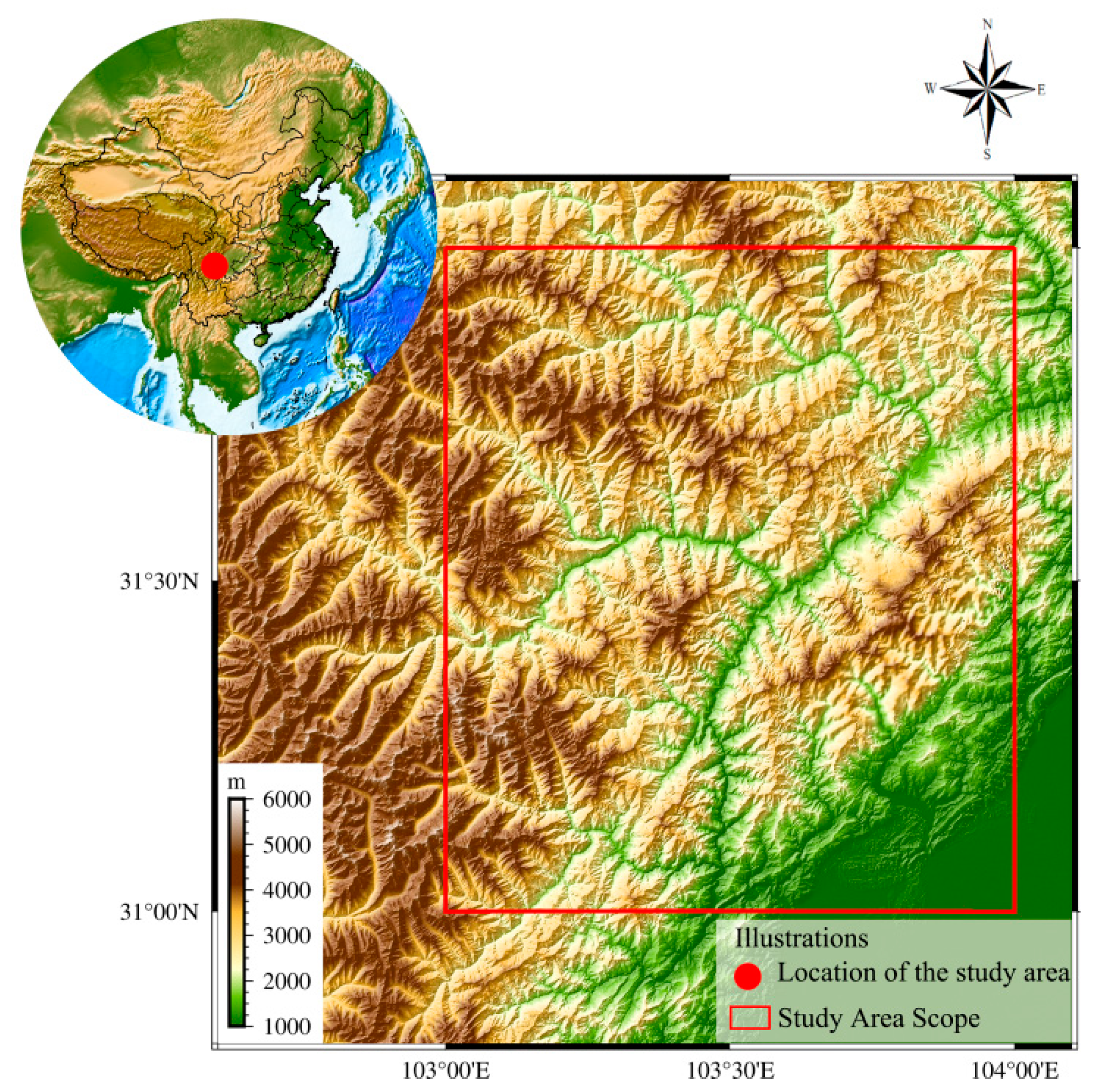
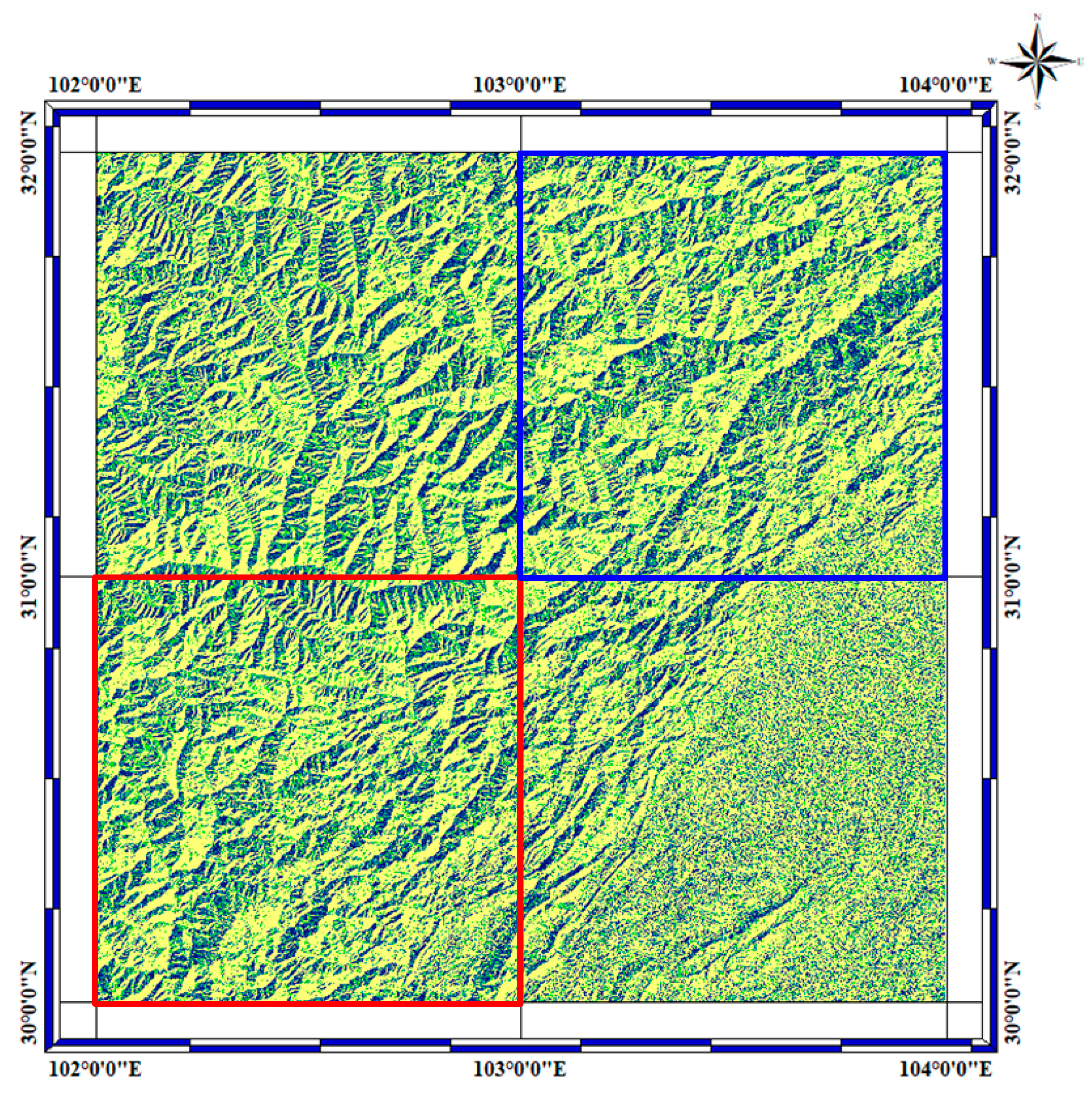
For the quantitative analysis, assuming that the DEM elevation error obeys normal distribution, the super-resolution reconstructed DEM can be measured by Root Mean Square Error (RMSE), Peak Signal-to-Noise Ratio (PSNR), Mean Absolute Error (MAE) and Median Absolute Deviation (MAD) [31]. The test dataset is selected from 24 DEM patches within the training area 31°N–32°N, 103°E–104°E. Super-resolution reconstructions are performed on the 24 DEM patches, and the RMSE, PSNR, MAE and MAD values are calculated for the results of the five DEM super-resolution reconstructions.

• RMSE

The error between the super-resolution reconstructed DEM and the true high-resolution DEM is measured by using the RMSE.

$$RMSE=\sqrt{\frac{1}{N}{\displaystyle \sum _{i=1}^N\Delta h_i^2}}$$

(23)

$N$ represents the number of samples, and $\Delta h_i^2$ represents the residual value of DEM elevation. As the value of RMSE becomes smaller, the objective evaluation algorithm predicts the subjective rating value more accurately, the performance of the model is better, and vice versa. The RMSE of the actual image is zero.

2.

PSNR

PSNR is a kind of evaluation index based on MSE. The unit of PSNR is dB, and larger values mean that the super-resolution reconstructed DEM is more similar to the original high-resolution DEM. Its calculation formula is shown below.

$$\begin{array}{cc}PSNR& =10\times {\log }_{10}(\frac{MA{X}_I^2}{MSE})\\ & =20\times {\log }_{10}(\frac{MA{X}_I}{\sqrt{MSE}})\end{array}$$

(24)

$$MSE=\frac{1}{mn}{\displaystyle \sum _{i=1}^m{\displaystyle \sum _{i=1}^n{(X_{ori(i,j)}-X_{res(i,j)})}^2}}$$

(25)

where $MA{X}_I$ represents the maximum value of the original image, Mean Square Error (MSE) is obtained by calculating the difference in elevation values between the super-resolution reconstructed DEM and the original DEM, $X_{ori(i,j)}$ denotes the true DEM, $X_{res(i,j)}$ denotes the super-resolution reconstructed DEM and m and n denote, respectively, the number of rows and columns of the DEM image.

3.

MAE

MAE is the absolute value of the mean error, and the MAE is calculated to better reflect the actual situation of the error in the DEM super-resolution reconstruction results.

$$\stackrel{\wedge }{\mu }=\frac{1}{N}{\displaystyle \sum _{i=1}^N|H_i-H_{ref}|}=\frac{1}{N}{\displaystyle \sum _{i=1}^N\Delta h_i}$$

(26)

$N$ represents the number of samples, $H_i$ represents the DEM elevation value after super-resolution reconstruction, $H_{ref}$ represents the elevation value of the original high-resolution DEM and $\Delta h_i$ represents the DEM elevation residual value.

In addition, considering that error accuracy is affected by outliers and the non-normal distribution of errors, robust statistical methods are considered in the evaluation of DEM accuracy.

4.

MAD

MAD is a robust statistic. For MAD, when there are a small number of outliers in the data, it does not affect the statistical results, avoiding the influence of outliers on the statistical accuracy of errors. $\Delta h_i$ denotes the DEM elevation residuals, and $m_{\Delta h}$ denotes the median of the elevation values. The calculation process is as follows.

$$MAD=media{n}_j(|\Delta h_j-m_{△h}|),$$

(27)

We quantify the analysis using four metrics: RMSE, PSNR, MSE and MAD. The results of the RMSE measure are shown in

Table 1. RMSE for the test regions.

RMSE (Unit Meter, the Lower the Better)
Method	Bicubic	SRCNN	VDSR	ZSSR	Ours
Average	8.48	8.30	8.09	7.02	6.65

. Smaller values of RMSE indicate a better reconstruction effect, and Figure 9 ais a visual representation of the results. As can be seen from the table, among the five DEM super-resolution reconstruction methods, the RMSE value of the reconstruction result of the DEM super-resolution reconstruction method based on a combination of internal and external learning that we propose is the smallest. Compared with the reconstruction results of the interpolation-based bicubic super-resolution reconstruction method, the reconstruction results are improve by 21.6%. Compared to the reconstruction results of the super-resolution reconstruction methods SRCNN and VDSR based on external learning in deep learning, the reconstruction results are improve by 19.9% and 17.8%, respectively. The reconstruction results improve by 5.3% compared to those of ZSSR, a super-resolution reconstruction method based on internal learning in deep learning.

The quantified results of PSNR are shown in

Table 2. PSNR for the test regions.

PSNR (in dB, the Higher the Better)
Method	Bicubic	SRCNN	VDSR	ZSSR	Ours
Average	53.94	54.14	54.36	55.60	56.07

. As the PSNR value becomes larger, the reconstruction effect becomes better. Figure 9 bis a visual representation of the results. From the table, it can be seen that, among the five DEM super-resolution reconstruction methods, the DEM super-resolution reconstruction method based on a combination of internal and external learning that we propose has the largest value of PSNR for the reconstruction results. Compared with the reconstruction result of the interpolation-based bicubic super-resolution reconstruction method, the reconstruction result is improve by 4.0%. Compared to the reconstruction results of the super-resolution reconstruction methods SRCNN and VDSR, which are based on external learning in deep learning, the reconstruction results improve by 3.6% and 3.2%, respectively. The reconstruction results improve by 0.9% compared to those of ZSSR, a super-resolution reconstruction method based on internal learning in deep learning.

The quantified results of MAE are shown in

Table 3. MAE for the test regions.

MAE (Unit Meter, the Lower the Better)
Method	Bicubic	SRCNN	VDSR	ZSSR	Ours
Average	5.72	5.73	5.42	4.98	4.73

. As the value of MAE becomes smaller, the reconstruction effect becomes better. Figure 9c is a visual representation of the results. From the table, it can be seen that, among the five DEM super-resolution reconstruction methods, our proposed DEM super-resolution reconstruction method based on a combination of internal and external learning has the smallest value of MAE for the reconstruction results. Compared with the reconstruction result of the interpolation-based bicubic super-resolution reconstruction method, the reconstruction result is improved by 17.3%. Compared to the reconstruction results of the super-resolution reconstruction methods SRCNN and VDSR based on external learning in deep learning, the reconstruction results are improved by 17.5% and 12.7%, respectively. The reconstruction results improve by 5.0% compared to those of ZSSR, a super-resolution reconstruction method based on internal learning in deep learning.

The quantified results of MAD are shown in

Table 4. MAD for the test region.

MAD (Unit Meter, the Lower the Better)
Method	Bicubic	SRCNN	VDSR	ZSSR	ours
Average	3.98	3.92	3.56	3.60	3.43

, where smaller values of MAD indicate better reconstruction results. Figure 9d is a visual representation of the results. From the table, it can be seen that, among the five DEM super-resolution reconstruction methods, our proposed internal-learning-based and external learning-based DEM super-resolution reconstruction method has the smallest value of MAD for the reconstruction results. The reconstruction result is improved by 13.8% compared to that of the interpolation-based bicubic super-resolution reconstruction method. Compared to the reconstruction results of the super-resolution reconstruction methods SRCNN and VDSR based on external learning in deep learning, the reconstruction results are improved by 12.5% and 3.7%, respectively. The reconstruction results improve by 4.7% compared to those of ZSSR, a super-resolution reconstruction method based on internal learning in deep learning.

4.4.2. Test Dataset Unrelated to the Training Set

In order to verify the generalization ability of the model and to avoid a correlation between the training and validation data, a region from 30°N to 31°N and from 102°E to 103°E is selected as the dataset outside the training area for the validation of the model. Similarly, we crop the region into 144 sheets of size 300 × 300 DEM patches to validate the generalization ability of bicubic interpolation, SRCNN, VDSR, ZSSR and our proposed new method in turn.

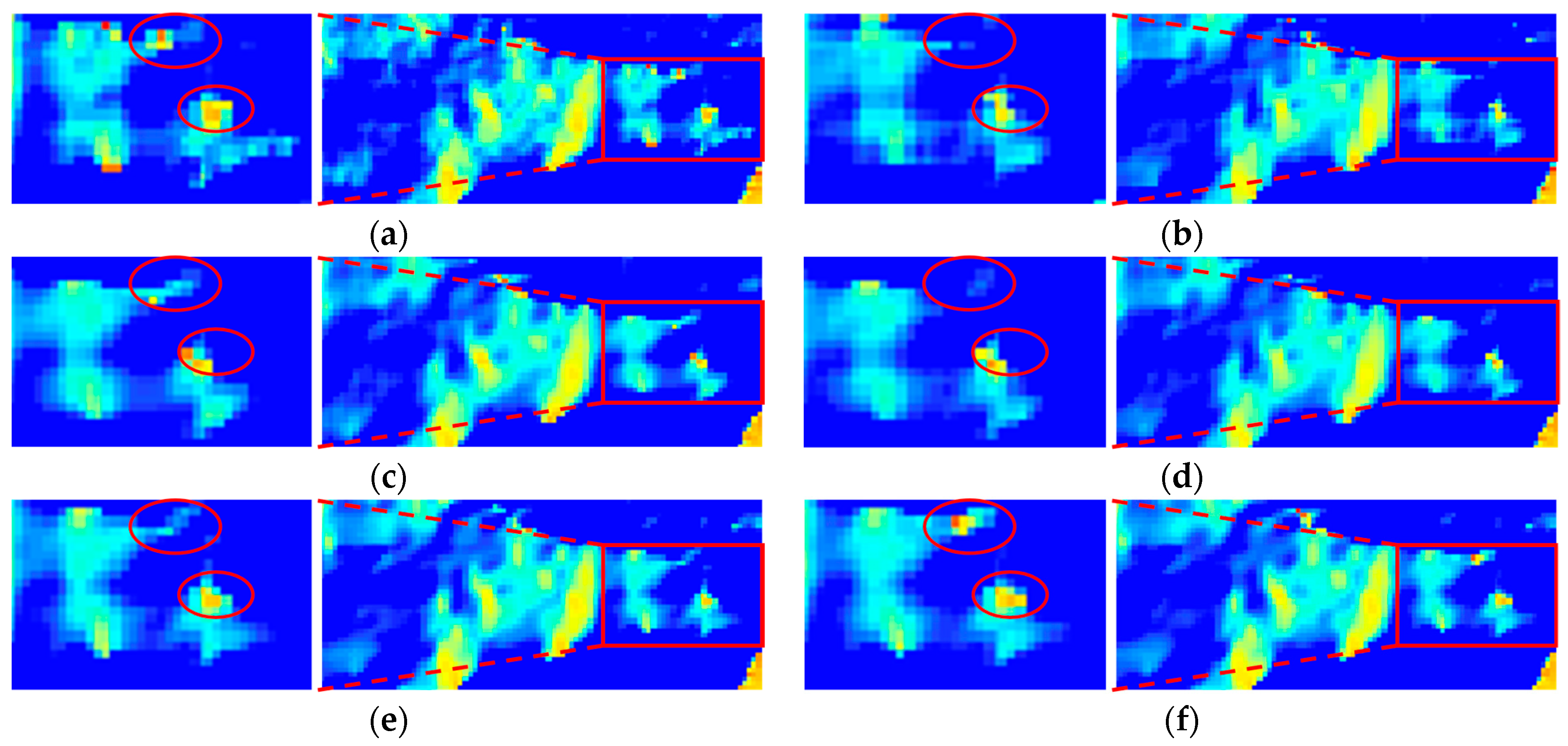
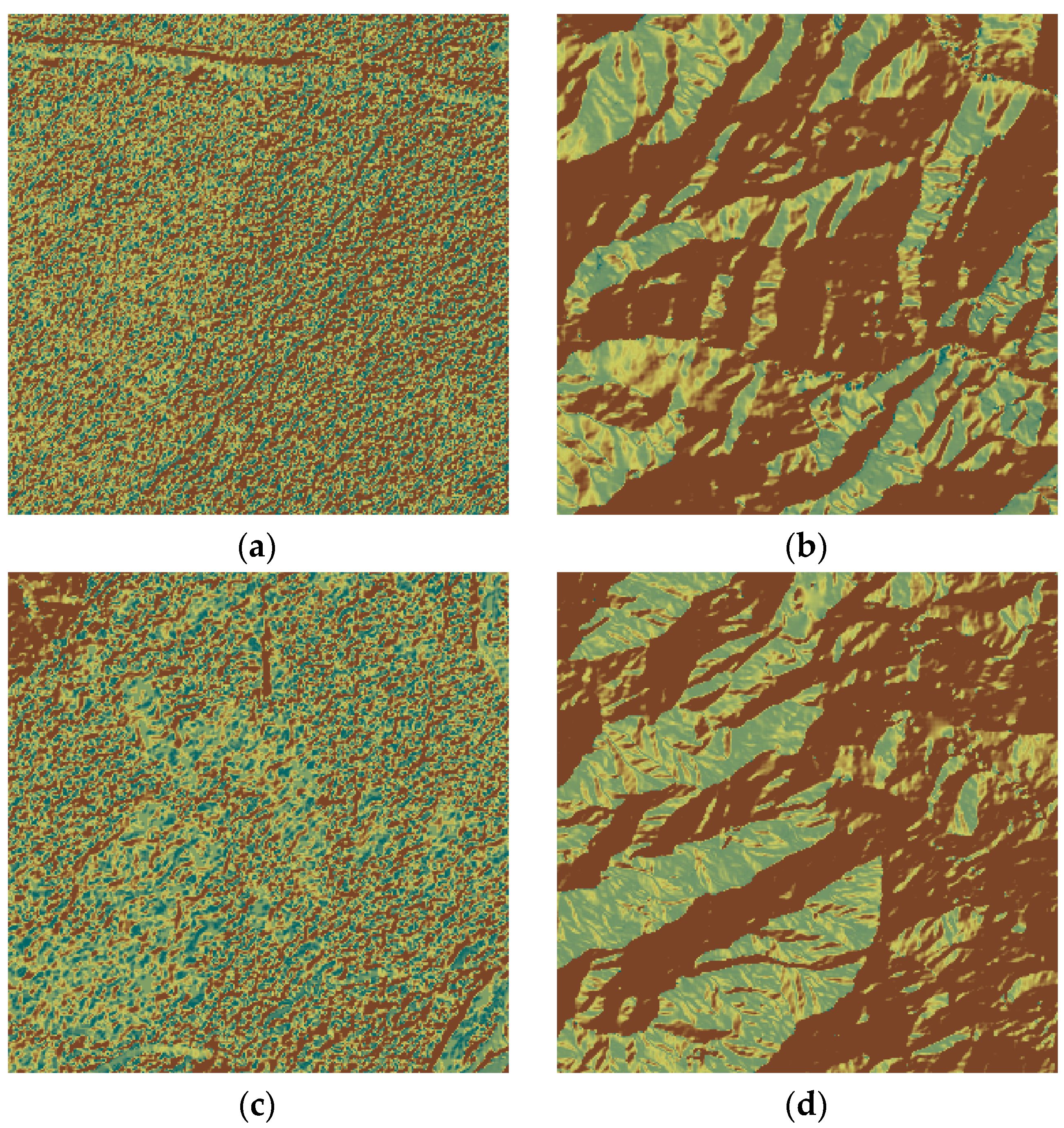
• Visual Analysis

As shown in Figure 10, Figure 10a represents the original high-resolution DEM, Figure 10b represents the result of super-resolution reconstruction of the DEM based on the bicubic interpolation method, Figure 10c represents the result of super-resolution reconstruction of the DEM based on the external learning super-resolution reconstruction method SRCNN, Figure 10d represents the result of super-resolution reconstruction of the DEM based on the external learning super-resolution reconstruction method VDSR, Figure 10e represents the result of super-resolution reconstruction of the DEM based on the internal learning super-resolution reconstruction method ZSSR and Figure 10f represents the result of super-resolution reconstruction of the DEM of our proposed combined internal learning and external learning super-resolution reconstruction method. From the visual evaluation we can see that the super-resolution reconstruction results of the interpolation-based bicubic DEM super-resolution reconstruction method lose more high-frequency information and show too smooth in the terrain. Among the learning-based super-resolution reconstruction methods, the super-resolution reconstruction results of SRCNN and VDSR have insignificant texture features and lose more detail information compared with the original high-resolution DEM. Among the learning-based super-resolution reconstruction methods, the results of super-resolution reconstruction by ZSSR are significantly better than the bicubic method, SRCNN and VDSR regarding their visual evaluation. Compared with several other DEM super-resolution reconstruction methods, our proposed combined internal learning and external learning DEM super-resolution reconstruction method is able to better recover the texture details of the DEM. The texture features are the richest compared to several other DEM super-resolution reconstruction methods and are closest to those of the original high-resolution DEM.

• Quantitative analysis

Similarly, we quantify the analysis using four metrics: RMSE, PSNR, MSE and MAD. From

Table 5. RMSE for the test regions.

RMSE (Unit Meter, the Lower the Better)
Method	Bicubic	SRCNN	VDSR	ZSSR	Ours
Average	7.86	6.78	7.96	5.88	5.58

,

Table 6. PSNR for the test regions.

PSNR (in dB, the Higher the Better)
Method	Bicubic	SRCNN	VDSR	ZSSR	Ours
Average	54.29	55.60	54.18	56.94	57.38

,

Table 7. MAE for the test regions.

MAE (Unit Meter, the Lower the Better)
Method	Bicubic	SRCNN	VDSR	ZSSR	Ours
Average	5.22	4.68	5.58	4.11	3.91

and

Table 8. MAD for the test regions.

MAD (Unit Meter, the Lower the Better)
Method	Bicubic	SRCNN	VDSR	ZSSR	Ours
Average	3.46	3.19	3.87	2.91	2.78

, it can be seen that, among the learning-based super-resolution reconstruction methods, the VDSR algorithm has poor network generalization capability for super-resolution reconstruction of the DEM. The VDSR algorithm is less effective for super-resolution reconstruction of the test set outside the training area, whereas ZSSR and the proposed method of combined internal and external learning for DEM super-resolution reconstruction in this paper achieve better reconstruction results for both the test area within and outside the training area. The test area is selected from 30°N–31°N, 102°E–103°E. The area is divided into 144 DEM patches, and the RMSE, PSNR, MAE and MAD values are calculated for each of these 144 DEM patches.

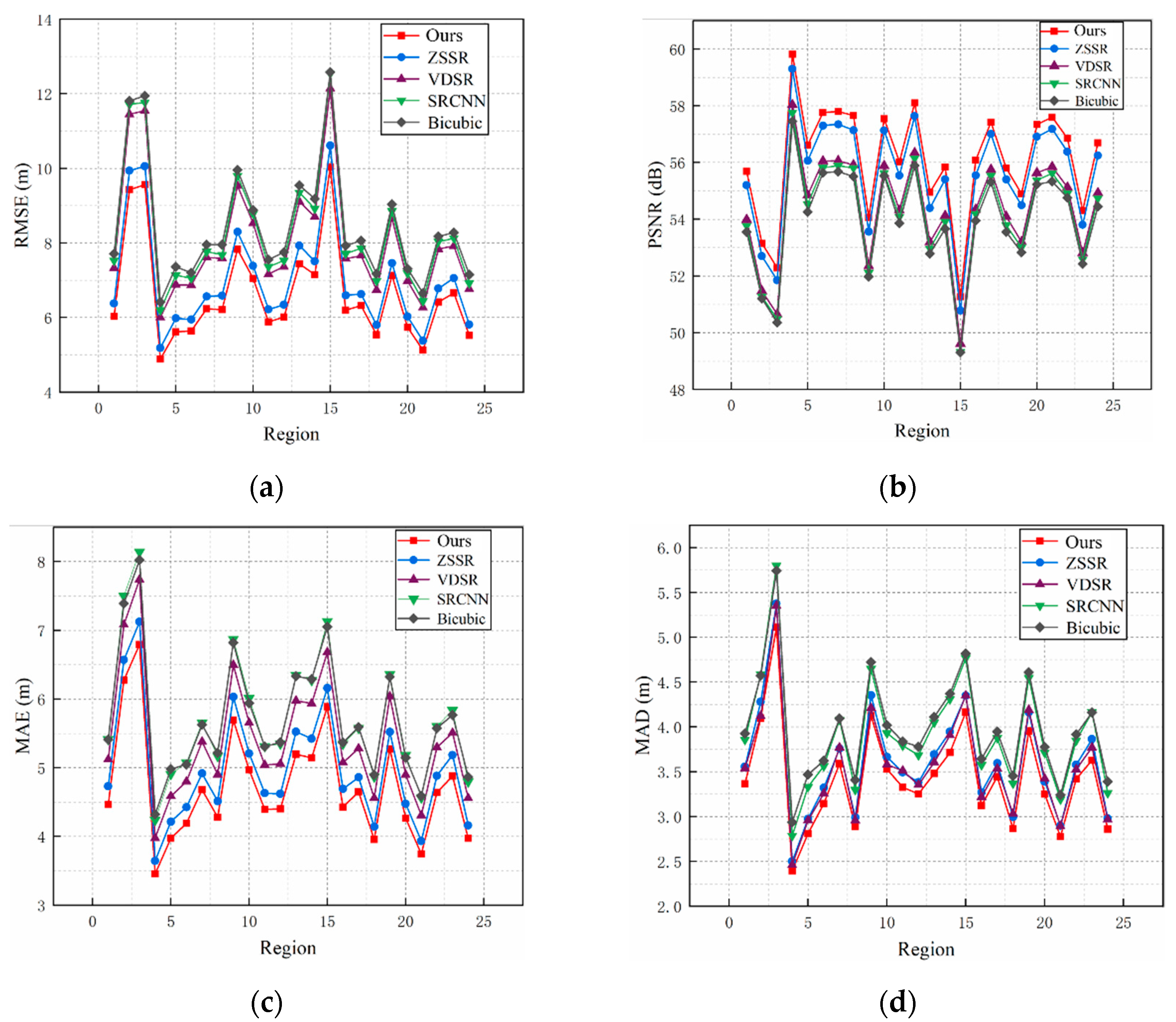
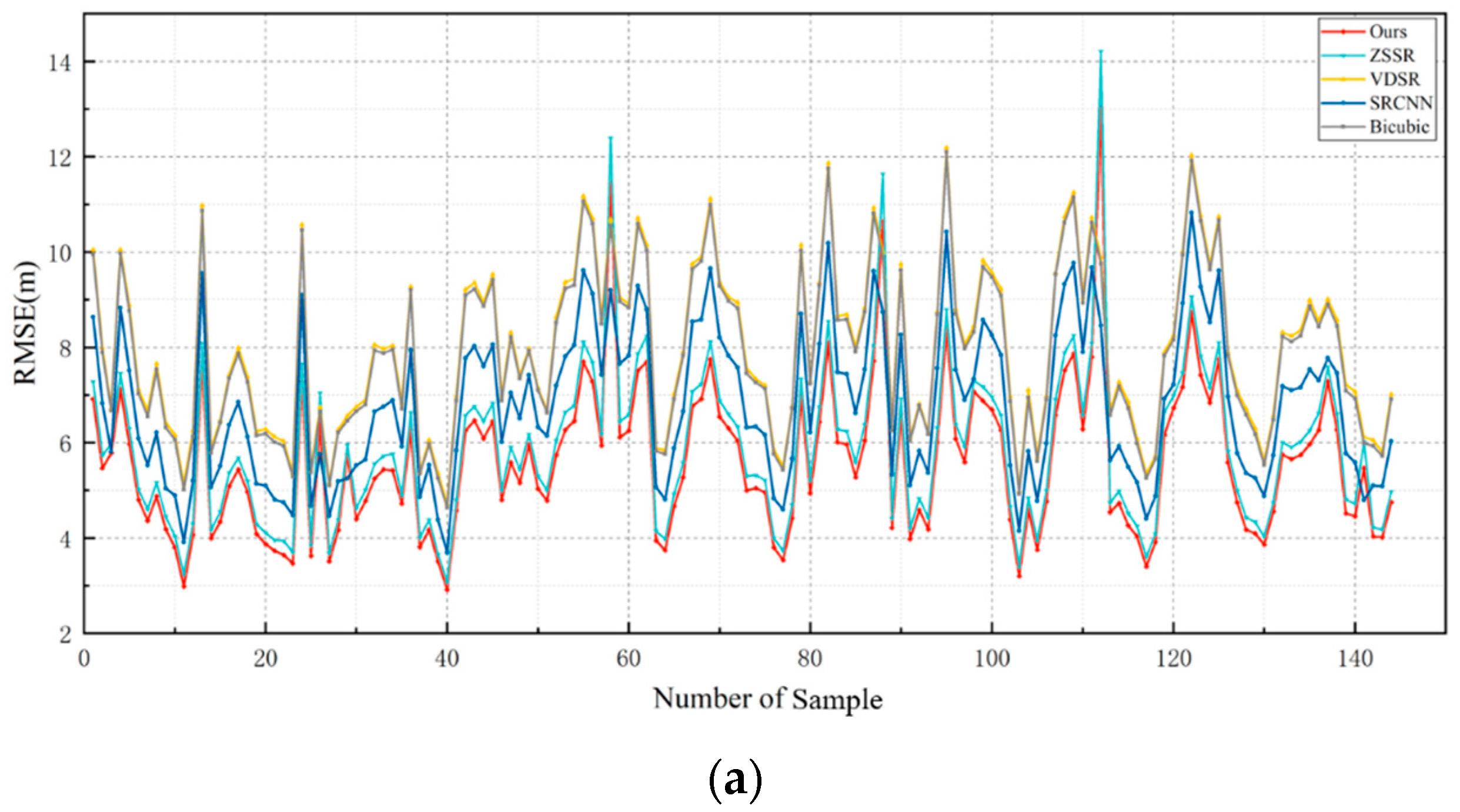
The test area is divided into 144 patches, and the average value of their RMSE results is shown in Table 5. Smaller values of RMSE indicate a better reconstruction effect, and Figure 11a is a visual representation of the RMSE values of the 144 DEM patches. As can be seen from the table, among the five DEM super-resolution reconstruction methods, our proposed DEM super-resolution reconstruction method based on a combination of internal and external learning has the smallest value of RMSE for the reconstruction result, with an improvement of 29.1% compared to the reconstruction result of the interpolation-based bicubic super-resolution reconstruction method. The reconstruction results are 17.7% and 30.0% better than those of SRCNN and VDSR, respectively, which are super-resolution reconstruction methods based on external learning in deep learning, and the results are 5.1% better than those of ZSSR, a super-resolution reconstruction method based on internal learning in deep learning.

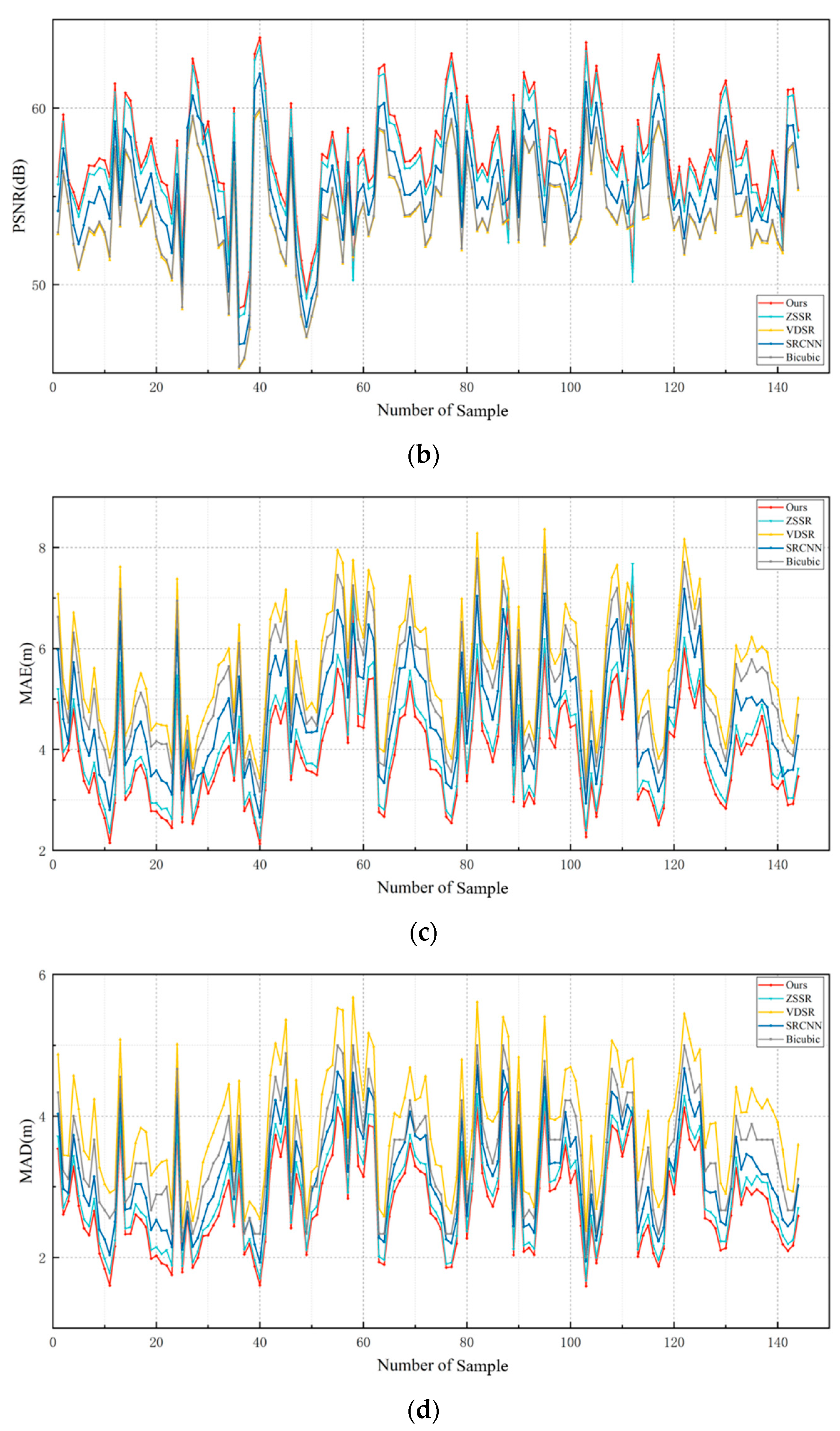
The average of the quantified results of the PSNR of the 144 DEMs in the test area is shown in Table 6. Larger PSNR values indicate a better reconstruction effect, and Figure 11b is a visual representation of the validation results for the 144 DEM patches. As can be seen from the table, among the five DEM super-resolution reconstruction methods, our proposed DEM super-resolution reconstruction method based on a combination of internal and external learning has the largest value of PSNR for the reconstruction results, with an improvement of 5.7% compared to the reconstruction results of the interpolation-based bicubic super-resolution reconstruction method and an improvement of 3.2% and 5.9% compared to the reconstruction results of the super-resolution reconstruction methods SRCNN and VDSR, respectively, which are based on external learning in deep learning. The reconstruction results are improved by 0.9% compared to those of ZSSR, a super-resolution reconstruction method based on internal learning in deep learning.

The average of the quantified results of MAE for the 144 DEMs in the test area is shown in Table 7. Smaller MAE values indicate a better reconstruction effect, and Figure 11c is a visual representation of the validation results for the 144 DEM patches. As can be seen from the table, among the five DEM super-resolution reconstruction methods, our proposed DEM super-resolution reconstruction method based on a combination of internal and external learning has the smallest value of MAE for the reconstruction results. Compared with the reconstruction results of the interpolation-based bicubic super-resolution reconstruction method, the reconstruction results of the super-resolution reconstruction methods SRCNN and VDSR, which are based on external learning in deep learning, improve by 25.0%, 17.0% and 30.4%, respectively. The reconstruction results of the super-resolution reconstruction method ZSSR, which is based on internal learning in deep learning, improve by 4.9%.

In order to avoid the influence of outliers and systematic errors on evaluation results, the robust estimation method of MAD is used to evaluate the 144 DEM patches in the test area, and the average value of the quantified results of their MAD is shown in Table 8. Smaller MAE values indicate better reconstruction. Figure 11d is a visual representation of the validation results for 144 small regions. As can be seen from the table, our proposed DEM super-resolution reconstruction method based on a combination of internal and external learning has the smallest value of MAD for the reconstruction results among the five DEM super-resolution reconstruction methods. The reconstruction results are improved by 20.0% compared to those of the interpolation-based bicubic super-resolution reconstruction method. Compared to the reconstruction results of SRCNN and VDSR, which are based on external learning in deep learning, the reconstruction results improve by 12.5% and 28.2%, respectively. The reconstruction results improve by 3.5% compared to those of ZSSR, a super-resolution reconstruction method based on internal learning in deep learning.

4.4.3. Performance Analysis of the Model for Different Terrain Features

Furthermore, in order to compare the performance of our proposed new method in mountainous and flat areas, two areas with distinct topographic features are selected for validation, as shown in Figure 12a,b represent flat areas and mountainous areas selected from the validation dataset within the training area, respectively. Figure 12c,d represent flat areas and mountainous areas, respectively, selected from the validation dataset outside the training area. The reconstruction-based bicubic method, the learning-based SRCNN and VDSR methods and the learning-based ZSSR method with external learning are selected for comparative analysis.

The values of the RMSE of the reconstructed results for each of the five methods in the two regions are shown in

Table 9. Values of RMSE for different super-resolution reconstruction methods in flat areas and mountainous areas of test datasets from the training region and outside the training region, respectively.

RMSE (Unit Meter, the Lower the Better)
	Bicubic	SRCNN	VDSR	ZSSR	Ours
Flat area	1.95	2.70	2.04	1.59	1.57
Mountainous area	8.48	7.29	7.69	6.65	6.27

. The results show that, in the flat area, our proposed new method improves 19.5% over the interpolation-based bicubic method, 41.9% over the learning-based SRCNN, and 23.0% over the VDSR method. The improvement over the internal learning ZSSR method of the learning-based methods is 1.3%, since in flat areas, where fewer texture features need to be learned, the improvement of our proposed new method is less. The results show that in the mountainous area, our proposed new method improves 26.1% over the interpolation-based bicubic method, 14.0% over the learning-based SRCNN, and 18.5% over the VDSR method. The improvement over the internal learning ZSSR method of the learning-based methods is 5.7%, since in flat areas, where fewer texture features need to be learned, the improvement of our proposed new method is less.

5. Discussion

From the visual analysis, both in the test area within the training area and with the test area outside the training area, it can be seen that the reconstructed textures and features in the super-resolution reconstruction results of our proposed method are better than those of the interpolation-based bicubic method, better than those of the deep learning-based external learning methods SRCNN and VDSR and better than those of the deep-learning-based internal learning method ZSSR. In addition, the reconstructed textures and features are closer to those of the original high-resolution DEM. In the quantitative evaluation, it can be seen that our proposed combined internal learning and external learning DEM super-resolution reconstruction method outperforms the deep-learning-based internal learning ZSSR method in all quantitative metrics of the reconstruction results. It is better than the SRCNN and VDSR methods based on the external learning of deep learning, and it is better than the interpolation-based bicubic method. In addition, by analyzing the reconstruction results for different landscape features, we find that our proposed new method not only gives good reconstruction in flat areas compared to several other reconstruction methods, but it also gives better enhancements in mountainous areas with significant textural features. The advantage of the method is that it makes full use of both internal and external information of the DEM, providing more accurate a priori information for the ill-posed problem of DEM super-resolution reconstruction. Although our experiments and analyses validate the effectiveness of our proposed combined internal and external learning method for DEM super-resolution reconstruction, there are still some details that deserve further discussion and investigation, which will be the main focus of our future work:

(1) Currently, we are building a data-to-data mapping relationship, so the question of how to combine physical-model-driven methods with data-driven methods will be the focus of our next research work.

(2) The super-resolution reconstruction algorithm of DEM plays a crucial role in the super-resolution reconstruction work of DEM, which we will explore next, defining different loss functions according to different terrain environments, attaching more a priori information and further improving network performance.

(3) We will further explore the impact of the choice of network parameters on the network model and the adaptive selection of parameters for different tasks of super-resolution reconstruction.

6. Conclusions

We introduce the internally learned ZSSR method into DEM super-resolution reconstruction and combine the existing externally learned DEM super-resolution reconstruction method to propose a new deep convolutional neural network for DEM super-resolution reconstruction work. The network learns detailed features from the DEM itself to obtain an initial estimated DEM sample. The initial estimated DEM sample dataset is then used as an externally learned low-resolution dataset to construct differential low-resolution DEM and high-resolution DEM data pairs with the original DEM dataset. External learning is then used to construct a global feature mapping of the DEM. It also makes full use of the complementary properties of internal and external learning to achieve joint learning of detailed features and global features of the DEM. More accurate a priori information is provided for the solution of the ill-posed inverse problem of super-resolution reconstruction. In addition, the model mines sample features through a deeper network and introduces residual learning to accelerate model convergence. Addressing the transfer of detailed features in the deeper network further improves the reconstruction performance of the network. The results of the visual and quantitative analysis show that the method is able to reconstruct the textures and features of the DEM significantly better than the super-resolution reconstruction method using interpolation and external learning alone. There are also improvements in visual evaluation and quantitative analysis over the super-resolution reconstruction method using internal learning alone, which is important for the super-resolution reconstruction of DEM.

References

1. Toutin, T. Impact of terrain slope and aspect on radargrammetric DEM accuracy. ISPRS J. Photogramm. Remote Sens. 2002, 57, 228–240. [Google Scholar] [CrossRef]
2. Yue, L. Research Ondem Fusion Blending Multisource and Multi-Scale Elevation Data; Wuhan University: Wuhan, China, 2017. [Google Scholar]
3. Liu, X. Airborne LiDAR for DEM generation: Some critical issues. Prog. Phys. Geogr. Earth Environ. 2008, 32, 31–49. [Google Scholar]
4. Li, Z.; Li, P.; Ding, D.; Wang, H. Global High-Resolution with Sparse Digital Elevation Model Research Progress and Prospects. Geomat. Inf. Sci. Wuhan Univ. 2018, 43, 1927–1942. [Google Scholar]
5. Kalimuthu, H.; Tan, W.N.; Lim, S.L.; Fauzi, M.F.A. Interpolation of low resolution Digital Elevation Models: A comparison. In Proceedings of the 2016 8th Computer Science and Electronic Engineering (CEEC), Colchester, UK, 28–30 September 2016; IEEE: Piscataway, NJ, USA, 2016; pp. 71–76. [Google Scholar]
6. Tang, G.; Na, J.; Cheng, W. Progress of Digital Terrain Analysis on Regional Geomorphology in China. Acta Geod. Et Cartogr. Sin. 2017, 46, 1570–1591. [Google Scholar]
7. Xu, Z. Research on Deep Learning Based Image Super-Resolution with Sparse Samples; Huazhong University of Science & Technology: Wuhan, China, 2019. [Google Scholar]
8. Hu, X. Research on Adaptive Image Super-Resolution; University of Science and Technology of China: Hefei, China, 2021. [Google Scholar]
9. Irani, M.; Peleg, S. Motion Analysis for Image Enhancement: Resolution, Occlusion, and Transparency. J. Vis. Commun. Image Represent. 1993, 4, 324–335. [Google Scholar] [CrossRef] [Green Version]
10. Stark, H.; Oskoui, P. High-resolution image recovery from image-plane arrays, using convex projections. J. Opt. Soc. Am. A 1989, 6, 1715–1726. [Google Scholar] [CrossRef] [PubMed]
11. Zeng, X.; Lu, H.; Zhang, C. Super Resolution Image Restoration Algorithm: Based on Wavelet and Interpolation. In Proceedings of the 2020 3rd World Conference on Mechanical Engineering and Intelligent Manufacturing (WCMEIM), Shanghai, China, 4–6 December 2020. [Google Scholar]
12. Jiao, D.; Wang, D.; Lv, H.; Peng, Y. Super-resolution reconstruction of a digital elevation model based on a deep residual network. Open Geosci. 2020, 12, 1369–1382. [Google Scholar] [CrossRef]
13. Xu, Z.; Wang, X.; Chen, Z.; Xiong, D.; Ding, M.; Hou, W. Nonlocal similarity based DEM super resolution. ISPRS J. Photogramm. Remote Sens. 2015, 110, 48–54. [Google Scholar] [CrossRef]
14. Zheng, X.; Xiong, H.; Yue, L.; Gong, J. An improved ANUDEM method combining topographic correction and DEM interpolation. Geocarto Int. 2016, 31, 492–505. [Google Scholar] [CrossRef]
15. Xu, Z.; Chen, Z.; Yi, W.; Gui, Q.; Hou, W.; Ding, M. Deep gradient prior network for DEM super-resolution: Transfer learning from image to DEM. ISPRS J. Photogramm. Remote Sens. 2019, 150, 80–90. [Google Scholar] [CrossRef]
16. Zhang, D.; China Electric Power Research Institute; Han, X.; Deng, C. Taiyuan University of Technology Review on the research and practice of deep learning and reinforcement learning in smart grids. CSEE J. Power Energy Syst. 2018, 4, 362–370. [Google Scholar] [CrossRef]
17. Kubade, A.; Sharma, A.; Rajan, K.S. Feedback Neural Network Based Super-Resolution of DEM for Generating High Fidelity Features. In Proceedings of the IGARSS 2020—2020 IEEE International Geoscience and Remote Sensing Symposium, Waikoloa, HI, USA, 26 September–2 October 2020; IEEE: Piscataway, NJ, USA, 2020; pp. 1671–1674. [Google Scholar]
18. Dong, C.; Loy, C.C.; He, K.; Tang, X. Image Super-Resolution Using Deep Convolutional Net-works. IEEE Trans. Pattern Anal. Mach. Intell. 2015, 38, 295–307. [Google Scholar] [CrossRef] [PubMed] [Green Version]
19. Argudo, O.; Chica, A.; Andujar, C. Terrain Super-resolution through Aerial Imagery and Fully Convolutional Networks. Comput. Graph. Forum 2018, 37, 101–110. [Google Scholar] [CrossRef]
20. Shin, D.; Spittle, S. LoGSRN: Deep Super Resolution Network for Digital Elevation Model. In Proceedings of the 2019 IEEE International Conference on Systems, Man and Cybernetics (SMC), Bari, Italy, 6–9 October 2019; IEEE: Piscataway, NJ, USA, 2019; pp. 3060–3065. [Google Scholar]
21. Zhang, H.; Quan, K.; Yang, Y.; Yang, J.; Chen, H.; Guo, W. Super-Resolution Reconstruction of Dem in Mountain Area Based on Deep Residual Network. Trans. Chin. Soc. Agric. Mach. 2021, 52, 178–184. [Google Scholar]
22. Kim, J.; Lee, J.K.; Lee, K.M. Accurate Image Super-Resolution Using Very Deep Convolutional Net-works. In Proceedings of the IEEE Conference on Computer Vision and Pattern Recognition 2016, Las Vegas, NV, USA, 1–26 June 2016. [Google Scholar]
23. Zontak, M.; Irani, M. Internal statistics of a single natural image. In Proceedings of the CVPR 2011, Colorado Springs, CO, USA, 20–25 June 2011; Institute of Electrical and Electronics Engineers (IEEE): Piscataway, NJ, USA, 2011; pp. 977–984. [Google Scholar]
24. Shocher, A.; Cohen, N.; Irani, M. Zero-Shot Super-Resolution Using Deep Internal Learning. In Proceedings of the 2018 IEEE/CVF Conference on Computer Vision and Pattern Recognition, Salt Lake City, UT, USA, 18–23 June 2018; pp. 3118–3126. [Google Scholar]
25. Liu, J.; Xue, Y.; Zhao, S.; Li, S.; Zhang, X. A Convolutional Neural Network for Image Super-Resolution Using Internal Dataset. IEEE Access 2020, 8, 201055–201070. [Google Scholar] [CrossRef]
26. Bo, Y. Study on Learning-Based Image Super-Resolution Method; Xidian University: Xi’an, China, 2019. [Google Scholar]
27. Glasner, D.; Bagon, S.; Irani, M. Super-resolution from a single image. In Proceedings of the 2009 IEEE 12th International Conference on Computer Vision, Kyoto, Japan, 29 September–2 October 2009; pp. 349–356. [Google Scholar]
28. Xiong, D. Research on Image Super Resolution Recontruction Methods Based on Edge Enhancement and Deep Learning; Huazhong University of Science and Technology: Wuhan, China, 2019. [Google Scholar]
29. Chen, Z.; Wang, X.; Xu, Z. Convolutional Neural Network Based Dem Super Resolution. Int. Arch. Photogramm. Remote Sens. Spat. Inf. Sci. 2016, 41, 247–250. [Google Scholar] [CrossRef] [Green Version]
30. Lim, B.; Son, S.; Kim, H.; Nah, S.; Lee, K.M. Enhanced deep residual networks for single image super-resolution. In Proceedings of the IEEE Conference on Computer Vision and Pattern Recognition Workshops (CVPRW), Honolulu, HI, USA, 21–26 July 2017; pp. 136–144. [Google Scholar]
31. Höhle, J.; Höhle, M. Accuracy assessment of digital elevation models by means of robust statistical methods. ISPRS J. Photogramm. Remote Sens. 2009, 64, 398–406. [Google Scholar] [CrossRef] [Green Version]
Figure 1. The linear constraint of low-resolution DEM patches on high-resolution DEM.
Remotesensing 14 02181 g001
Figure 2. The processing flow of the feature reconstruction module.
Remotesensing 14 02181 g002
Figure 3. The processing flow of the reconstruction module.
Remotesensing 14 02181 g003
Figure 4. Network structure.
Remotesensing 14 02181 g004
Figure 5. Overview of the study area.
Remotesensing 14 02181 g005
Figure 6. Network process.
Remotesensing 14 02181 g006
Figure 7. Distribution of the training and testing areas.
Remotesensing 14 02181 g007
Figure 8. Detailed textures of the original DEM and the DEM after super-resolution reconstruction of the DEM using different methods: (a) The texture details of the original DEM; (b) The texture details of DEM after DEM super-resolution reconstruction using the bicubic method; (c) The texture details of DEM after DEM super-resolution reconstruction using SRCNN with external learning in deep learning; (d) The texture details of DEM after DEM super-resolution reconstruction using VDSR with external learning in deep learning; (e) The texture details of the DEM after DEM super-resolution reconstruction using internal learning-based ZSSR in deep learning; (f) The texture details of the DEM after DEM super-resolution reconstruction using our proposed new method of combined internal and external learning.
Remotesensing 14 02181 g008
Figure 9. Quantitative results of different methods for the same region: (a) The visualization of the RMSE indicator; (b) The visualization of the PSNR indicator; (c) The visualization of the MAE indicator; (d) The visualization of the MAD indicator.
Remotesensing 14 02181 g009
Figure 10. Comparison of the results of the original high-resolution DEM with the five DEM super-resolution reconstruction methods: (a) Original, (b) Bicubic, (c) SRCNN, (d) VDSR, (e) ZSSR, (f) Ours.
Remotesensing 14 02181 g010
Figure 11. Quantitative results for the test area outside the training area: (a) RMSE value of the test area; (b) PSNR value of the test area; (c) MAE value of the test area; (d) MAD value of the test area.
Remotesensing 14 02181 g011aRemotesensing 14 02181 g011b
Figure 12. (a) A flat area in the test area within the training area; (b) A mountainous area in the test area within the training area; (c) A flat area in the test area outside the training area; (d) A mountainous area in the test area outside the training area.
Remotesensing 14 02181 g012