Abstract
Solar-induced chlorophyll fluorescence (SIF), when used as a proxy for plant photosynthesis, can provide an indication of the photosynthesis rate and has the potential to improve our understanding of carbon exchange mechanisms within an ecosystem. However, the relationships between SIF and vegetation indices (VIs) operating within different ecological contexts and the effect of other environmental factors on SIF remain unclear. This study focused on three ecosystems (cropland, forest, and grassland), with different ecological characteristics, located in Northeast China. These areas provide case studies where numerous relationships can be explored, including the correlations between the Orbiting Carbon Observatory-2 (OCO-2) SIF and MODIS products, meteorological factors, and the differences in the relationships between the three different ecosystems. Some interesting results and conclusions were obtained. First, in different ecosystems, the relationships between SIF and MODIS products show different correlations, whereby the enhanced vegetation index (EVI) has a close relationship with SIF in all the three ecosystems of forest, cropland, and grassland. Second, forest-type ecosystems appear to be sensitive to changes in daily temperature, whereas cropland and grassland areas respond more closely to changes in previous 16-day daily minimum temperature. Compared with forest and cropland areas, grasslands were more sensitive to precipitation (although the R2 value was small). Third, different ecosystems have different mechanisms of photosynthesis. Hence, we suggest that it is better to use SIF in areas exhibiting different ecological characteristics, and different models should be employed while simulating SIF.
1. Introduction
Traditional vegetation indices (VIs) derived from remotely sensed data have been used effectively in several previous studies in the field of terrestrial ecosystem research [1,2,3]. However, these ‘greenness’-based VIs (e.g., normalized difference vegetation index (NDVI), enhanced vegetation index (EVI), and leaf area index (LAI)) only capture changes in vegetation canopy reflectance attributable to leaf loss or chlorophyll content [4]. Furthermore, some of these VIs can experience a saturation effect in cases where the target vegetation is particularly dense. As an alternative, solar-induced chlorophyll fluorescence (SIF) has been widely used in studies concerned with monitoring vegetation physiology, given its functional connection with plant photosynthesis [5,6,7,8]. The terrestrial ecosystem carbon cycle has been studied for decades by using time serious remote sensing data, as the cycle is directly related to the actual photochemistry of plants [9,10].
SIF is a faint chlorophyll fluorescence signal (representing less than 5% of the total light absorbed by plants), which is emitted by the dissipation of excess light during the absorption process [7,11,12]. SIF has been widely proposed as a proxy measurement of plant photosynthesis and as an input for terrestrial primary productivity models [7]. A closed linear relationship between SIF and gross primary production (GPP) (SIF–GPP) has been evidenced both at regional and at global scales [12,13,14,15], as SIF contains information on both the absorption of photosynthetically active radiation (PAR) and energy partitioning in photosystems [4,16]. Gu et al. [17] argued that in the cases of both C3 and C4 plants, the relationship between SIF and GPP is nonlinear. A strongly non-linear relationship between SIF and GPP was also found in temperate evergreen needle leaf forests, likely due to the different responses to absorbed photosynthetically active radiation (APAR) and air temperature particular to the plant species found in these areas [18]. This non-linear relationship may also be due to the lack of saturation effect observed in SIF under conditions of high light and dense vegetation, whereas VIs such as GPP are susceptible to saturation effects [17]. The differences in fundamental processes between SIF and GPP may also be a contributing factor [19].
Since SIF is not susceptible to saturation effects [20], there has been extensive research concerned with densely vegetated areas, such as forests and croplands [6,12,21]. The close linear or non-linear relationship between SIF and canopy GPP can be used to monitor vegetation photosynthesis, as well as the carbon cycle, at regional and global scales [18,22]. SIF also offers advantages in the study of vegetation phenology because it is sensitive to both the initial and final stages of photosynthesis, which are not mechanistically linked to leaf greenness [6,23]. SIF may better detect water stress and temperature stress in vegetation than VIs, which rely on the spectral reflectance signatures produced by changes in canopy structure [24]. In tropical rainforests, SIF decreases in the dry season, resulting in a decrease in GPP, which indicates that SIF varies with water availability and that drought weakens the ability of vegetation to engage in carbon fixation [4]. A meta-analysis also revealed that drought stress, accompanied by a decrease in SIF, as well as heat stress (which is typically associated with drought stress), usually causes a decline in SIF [25]. Kimm et al. [24] used soybean plants in an experiment designed to explore the response of SIF yield to temperature stress. Experimental results indicated that, beyond a certain threshold, yield decreased as temperatures increased, revealing a negative correlation in instances where temperature exceeded the growth optimum. They also found that the SIF value was affected by canopy structure.
Hitherto, SIF data have been derived from numerous sensors. These include devices mounted on the Greenhouse Gases Observing Satellite (GOSAT), the Global Ozone Monitoring Experiment 2 (GOME-2) instrument, carried aboard the MetOp-A (Meteorological Operational Satellite A), the Scanning Imaging Absorption spectrometer for Atmospheric CHartograhY (SCIAMACHY) onboard Envisat, the Orbiting Carbon Observatory-2 and -3 (OCO-2 and OCO-3), and the TROPOspheric Monitoring Instrument (TROPOMI). Although none of these satellite missions were originally designed for SIF mapping, they provided the initial datasets that revealed the feasibility of satellite SIF retrievals, both at a coarse spatial resolution or at footprint level. Progressive advances in satellite technology and improvements in satellite SIF retrieval technology will allow for a more direct estimation of transpiration and play a more significant role in understanding the carbon cycle of terrestrial ecosystems as a whole.
Frankenberg et al. [11] derived a measurement of average global annual SIF at 755 nm with a spatial resolution of 2° × 2° using GOSAT data. To obtain higher spatial and temporal resolutions and a continuous SIF dataset, many researchers use MODIS products and meteorological data, employing linear regression techniques to simulate global or regional SIF [12,26,27,28,29]. Satisfactory results have been obtained by such means. Different plant species typically exhibit different photosynthetic characteristics and different light use efficiencies (LUE) [22]. However, in previous studies, the photosynthetic characteristics of different ecosystems have not been considered while performing SIF simulations.
This research aims to (1) understand the seasonal trends of SIF for the ecosystems of cropland, forest, and grassland, (2) identify and quantify the relationships between VIs and SIF at both regional and footprint scales, (3) understand how meteorological factors affect SIF in different vegetation types, and (4) estimate the accuracy of former SIF products of different vegetation types and then compare the difference.
2. Materials and Methods
2.1. Study Region
To explore the relationships of SIF and vegetation indices and the sensitivity of SIF to meteorological data in different ecosystems, three typical ecosystems in Northeast China, forest, grassland, and cropland, were selected in this research. The study region is located in northeastern China and contains the three provinces of Heilongjiang, Jilin, and Inner Mongolia (111°04′17″–130°44′56″ E, 41°15′10″–53°35′11″ N). It is bounded by Russia to the north and Mongolia to the west.
The Greater and Lesser Khingan Mountains represent the forest ecosystems, the Songnen Plain represents the cropland ecosystem, and Hulunbuir grasslands and Xilin Gol grasslands represent the grassland ecosystems. These land cover types, with a 30 m resolution [30], were selected to explore the different responses of land cover types to changes in SIF (Figure 1).
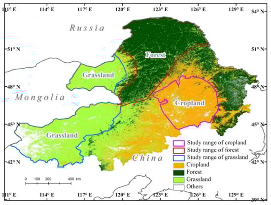
Figure 1.
Geographic location of the study area consisting of forest, cropland, and grassland ecosystems (Reference. frame: GCS_WGS_84, EPSG: 4326).
The Greater Khingan Mountains are part of the coniferous forests of northern Eurasia and constitute the largest virgin forest in China. The zonal vegetation is typical taiga type composed principally of Dahurian larch (Larix gmelinii), deciduous broadleaf birch (Betula platyphylla), and aspen (Populus davidiana and Populus suaveolens) [6,8]. Elevations in the area range from 260 m to 1700 m. The Greater Khingan Mountains experience a cold temperate and continental monsoon climate with an annual average temperature of −2.8 °C and a mean annual precipitation of 350–500 mm [31,32].
The cropland ecosystem is located in the central Songnen Plain, which is one of the ‘black soil regions’ of the world. The Songnen Plain is one of the most important grain production areas in China, and this region has the largest acreage of corn and also small area of rice. Mean annual precipitation in the Songnen Plain is 350–700 mm. The area typically experiences mean temperatures in the range of 21–26 °C in the month of July and −24 to 9 °C in January.
The Hulunbuir and Xilin Gol grasslands, which are part of the Inner Mongolia typical steppe, have an annual mean temperature range from −2 to 26 °C and have a mean annual precipitation of approximately 300 mm [33].
2.2. OCO-2 SIF Data
The OCO-2 satellite was launched into a polar orbit on 2 July 2014. It is a National Aeronautics and Space Administration (NASA) satellite, and is specially designed to monitor CO2 concentrations in the atmosphere [12]. The OCO-2 SIF product is an unexpected but critical complementary by-product of OCO-2′s primary mission target [14]. The OCO-2 spectrometer measures the spectra in the O2 A band, with far-red SIF being retrieved at wavelengths of 757 and 771 nm (SIF757 and SIF771) based on the infilling of the Fraunhofer lines at 13:36 local time. Each second, OCO-2 acquires 24 data points with a footprint of 1.3 km × 2.25 km. The precision of the OCO-2 SIF is better than 0.05 W m−2 sr−1 μm−1 with just a single detector footprint in the ideal case of an entirely opaque Fraunhofer line [8,34,35].
The OCO-2 SIF Lite data consist of daily points that contain both ‘value’ and location information, as well as a description of statistical bias and cloud cover. In this study, we used SIF data derived from the OCO-2 Lite products (V9r) collected during the period 2015–2020. The data were sourced from the NASA Earth Data archive (https://earthdata.nasa.gov/ accessed date: 15 July 2019). Many researchers have argued that SIF757 is more accurate than SIF771 because it is closer to the spectrum peak [35,36]. Hence, we opted to use SIF757 data in this research.
2.3. MODIS EVI, FPAR, and LAI Products
The MODIS products of EVI, the fraction of photosynthetically active radiation (FPAR), and LAI were used in this study. There are close relationships among MODIS-derived indices, but these indices reflect plant photosynthesis in different ways, and different MODIS indices were used to model SIF for different aims. MODIS-derived NDVI has been widely employed in terrestrial ecosystem studies. However, due to the possible implications posed by the saturation effect [12,21], we opted to use EVI as a means of gauging change in the vegetation cover in forest, cropland, and grassland areas. MODIS GPP was not considered in this study because there was no significant relationship between MODIS GPP and OCO-2 SIF in forest areas [12].
LAI provides a measurement of the one-sided green leaf area present per unit ground area in broadleaf canopies and half the total needle surface area per unit ground area in coniferous canopies. The fraction of photosynthetically active radiation (FPAR) measure is the fraction of photosynthetically active radiation (400–700 nm) absorbed by green vegetation [37].
The EVI was extracted from the 16-day composite MOD13A1 product, with a spatial resolution of 500 m. The LAI and FAPAR were extracted from the 8-day composite MOD15A2H product, with a spatial resolution of 500 m. These MODIS products were downloaded from the NASA Land Processes Distributed Active Archive Center (LP DAAC).
2.4. Meteorological Data
In this study, temperature data, including daily mean temperature, daily maximum temperature, daily minimum temperature, and daily mean precipitation data, were obtained from the National Meteorological Information Center (NMIC, http://data.cma.cn/, accessed date: 12 March 2019). The weather stations within each vegetation type were selected to represent the meteorological data.
2.5. Modeled SIF Products Used in This Study
To check the accuracy of the modeled SIF product for different ecosystems, a global OCO-2 SIF dataset (GOSIF) [26] and high-resolution global contiguous SIF (HRGCSIF) [38] were used in this study.
GOSIF is a dataset with a 0.05-degree spatial resolution and an 8-day temporal resolution. It was derived from MODIS products and meteorological reanalysis data using a data-driven approach. The GOSIF dataset can be download freely from https://globalecology.unh.edu/data/GOSIF.html, accessed date: 20 September 2019.
HRGCSIF is also a dataset with a 0.05-degree spatial resolution, but which has a 16-day temporal resolution. This product was produced by training an artificial neural network (ANN) on the OCO-2 observations for SIF and MODIS seven-band surface reflectance. HRGCSIF can be download from https://daac-news.ornl.gov/content/high-resolution-global-contiguous-sif-estimates-v2, accessed date: 20 September 2019.
2.6. Data Processing
In order to temporally standardize the various data products used, SIF, daily temperature, and precipitation were grouped into 16-day datasets. The 8-day LAI and FPAR datasets were compiled into 16-day datasets using the maximum value composition technique [39].
This study explores the response of SIF in different ecosystems at both the regional and footprint scales. At the regional scale, we calculated the regional average values of SIF, EVI, FPAR, and LAI, as well as the averages of the various meteorological factors considered for each ecosystem, and scatter plots were subsequently plotted. To measure the strength of any correlations of SIF–EVI, SIF–FPAR, and SIF–LAI at the footprint scale, we randomly selected 100 SIF points in each 16-day growing period (from 22 April to 15 October) representing the cropland, forest, and grassland ecosystems. The selected 100 SIF points were buffered with a 2 km radius, and we then extracted the averaged values of EVI, FPAR, and LAI within the circle and the scatter plots were plotted accordingly. We ensured that the spatial interval between random points was greater than 10 km to eliminate the risk of spatial autocorrelation.
In order to ensure that the relationships identified between the SIF and MODIS products in each sub-region were not biased or affected by other land cover types, the latter were selected as described in Table 1 using the 2020, 30 m resolution Global Land Cover with Fine Classification System (GLC_FCS30-2020, https://zenodo.org/record/4280923#, accessed date: 10 August 2021).

Table 1.
Classification system of cropland, forest, and grassland used in this study.
To de-seasonalized the time series of temperature and SIF, the method of value minus multi-year mean value was used before we calculated the relationships of them.
3. Results
3.1. Trend of SIF in Different Ecosystems
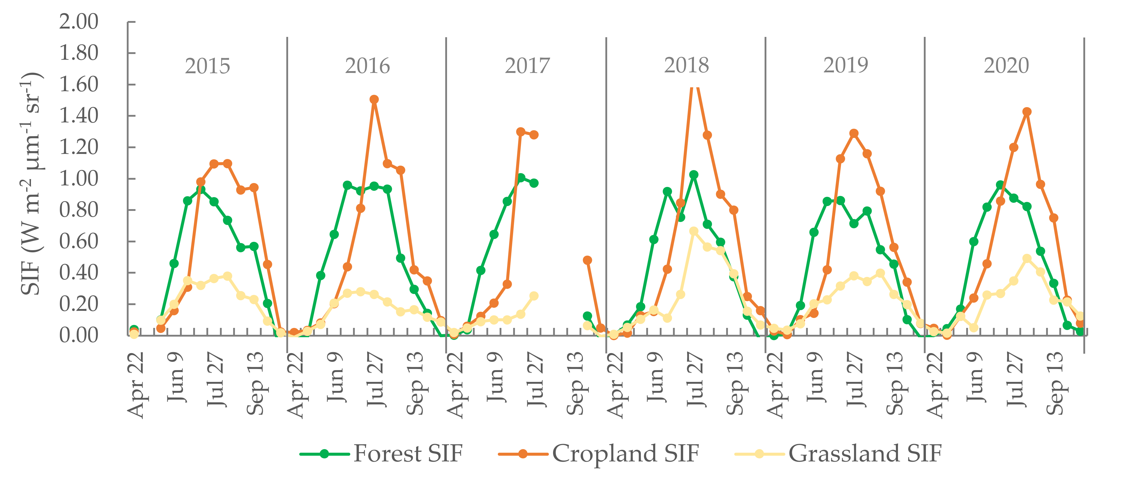
Evident periodical changes in forest, cropland, and grassland are shown in Figure 2. As observed, the wave crests corresponding to grassland are of a lower amplitude than those of forest or cropland. The highest values recorded and, consequently, the highest amplitude data peaks visible in Figure 2 corresponded to cropland. Sarvia et al. [40] analyzed how climate change affects vegetation phenology (derived from maximum annual NDVI) in different ecosystems and found that forest and agriculture show different phenological trends. In the latter case, peak SIF values were recorded in late July or early August each year. With regard to the peak values of the three land cover types, the maximum SIF value occurred in croplands and the minimum value in grasslands. During the initial stages of photosynthesis, the forest ecosystem yielded higher SIF values than the cropland areas. However, by July, cropland SIF values had overtaken the forest SIF values. Turner et al. [41] also obtained similar SIF trends of evergreen forest, cropland, and grassland to this study. Furthermore, they also found double peaks in the seasonality of SIF due to two ecosystems that are out of phase with each other. However, in this study, the selected forest, cropland, and grassland were nearly pure ecosystems and no obviously double peak of SIF was found.
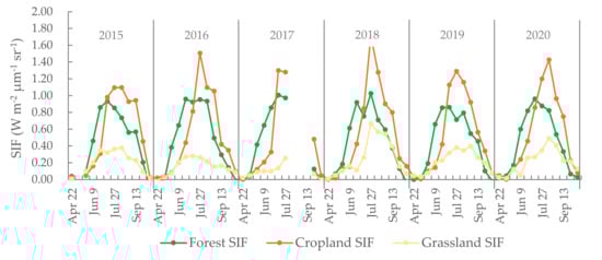
Figure 2.
MSixteen-day SIF of cropland, forest, and grassland from 2015 to 2020. The missing data for SIF in May 2015 and August 2017 are because the OCO-2 orbit did not cover the study region.
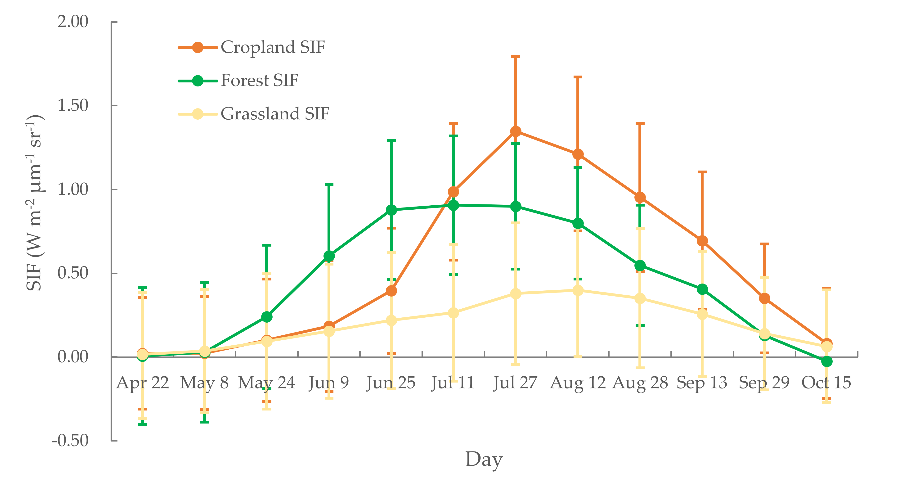
We also calculated the multi-year average SIF values for each 16-day period. These calculations notably depict the SIF changes that occur within a growing season (Figure 3). The SIF values for the forest ecosystem increase from May 8, reaching a peak at the beginning of July, and then subsequently decrease. During the intermediate period, i.e., from late June until the end of July, SIF values remained high. For cropland, SIF values reach a peak value on 27 July or 12 August. The grassland ecosystem exhibited comparatively gentle changes in SIF throughout the growing season. We also found that the peak SIF value of cropland was higher than that of forest, the former surpassing the latter in early July. These differences were primarily because of the different responses of SIF to the canopy structure of the different photosynthesis processes and mechanisms (especially for C3 and C4 plants) in different ecosystems [14].

Figure 3.
Multi-year averages of 16 d SIF values for cropland, forest, and grassland ecosystems.
3.2. Relationship between SIF and MODIS at Regional Scale
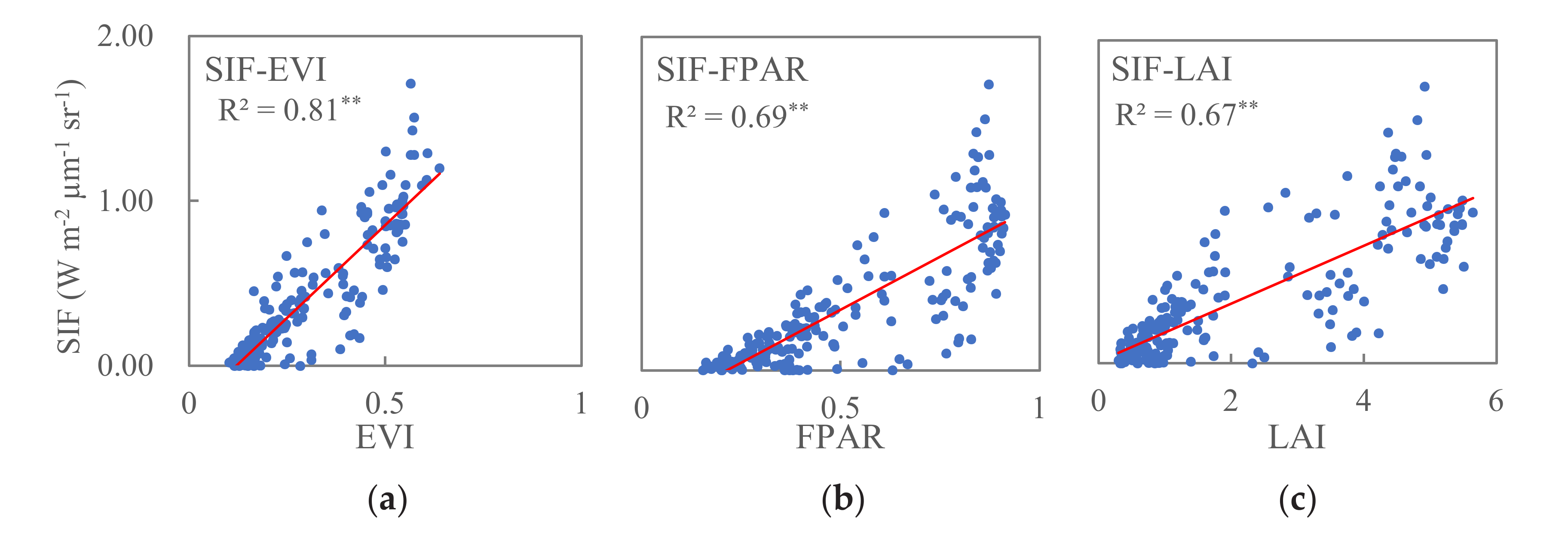
At the regional scale, the relationships between SIF and EVI (SIF–EVI), SIF and FPAR (SIF–FPAR), and SIF and LAI (SIF–LAI) for the three vegetation type zones are shown in Figure 4. Linear, exponential, power, and quadratic models were tried for each scatter plot, and we then selected the best fit one. An F-test was used to test the significance of the regression models. Statistically significant relationships were found between SIF and EVI (R2 = 0.81, p < 0.001), SIF and FPAR (R2 = 0.69, p < 0.001), and SIF and LAI (R2 = 0.67, p < 0.001), indicating that regional scale vegetation canopy greenness can reflect increasing vegetation photosynthetic activity. SIF–EVI has a higher correlation coefficient than SIF–FPAR and SIF–LAI.
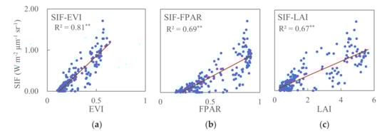
Figure 4.
Relationships of SIF–EVI (a), SIF–FPAR (b), and SIF–LAI (c) in the study region, where ** means p < 0.001.
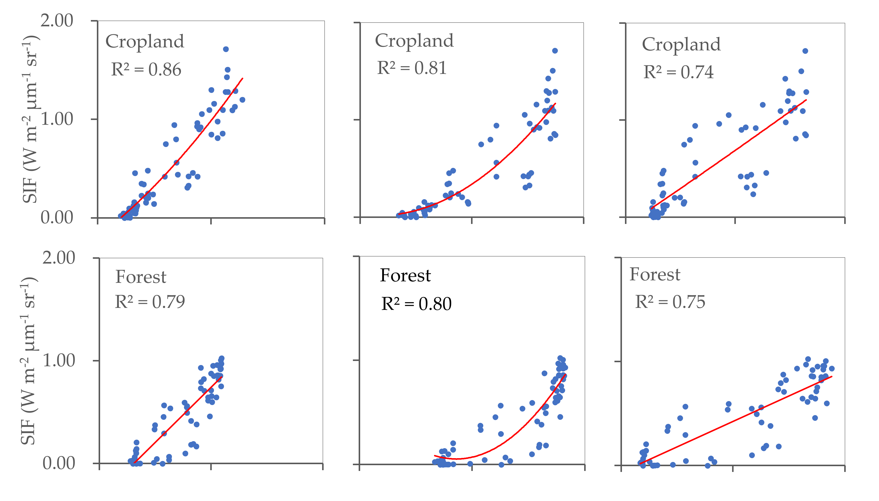
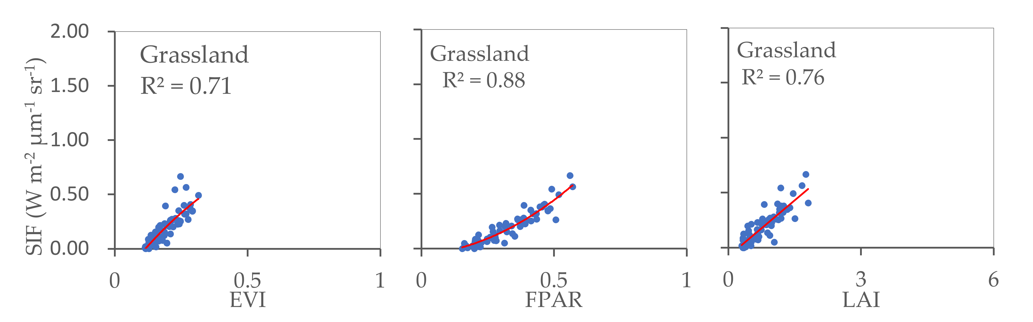
The relationships identified between SIF and EVI, SIF and FPAR, and SIF and LAI for cropland, forest, and grassland were also calculated (Figure 5). The results reveal significant correlations in all three land cover types considered, with R2 values ranging between 0.71 and 0.88 (p < 0.001). This indicates that in each land cover type, vegetation greenness and photosynthetic activity are consistently related at a regional scale. The strongest relationship was observed between SIF and EVI in cropland, whilst grassland yielded the strongest SIF–FPAR relationship. The R2 values calculated for SIF–LAI were similar for cropland, forest, and grassland.
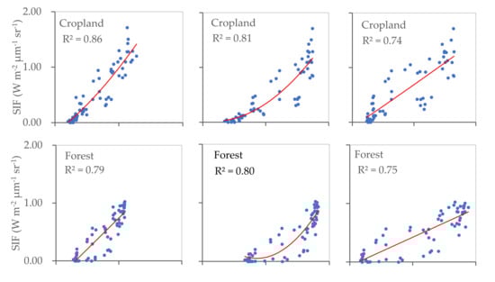
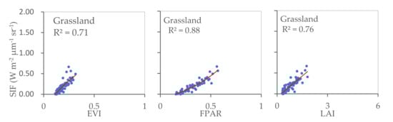
Figure 5.
Relationships between SIF and EVI, SIF and FPAR, and SIF and LAI for cropland, forest, and grassland areas (p < 0.001).
3.3. Relationship between SIF and MODIS at OCO-2 Footprint Level
For forest, cropland, and grassland areas, scatter plots were drawn from SIF points for each 16-day period and the corresponding spatial values of EVI, FPAR, and LAI at a footprint level. Statistically significant correlations were obtained for SIF–EVI in cropland, forest, and grassland areas. The largest R2 value was observed in cropland, followed by grassland, and finally forest areas (Table 2). In the case of SIF–FPAR, although significant correlations were obtained for three land cover types, the R2 value corresponding to the forest areas was lower than 0.1. With regard to SIF–LAI, no R2 value greater than 0.1 was found for any of the three land cover types; this indicates that if SIF was taken as a dependent variable, EVI could explain 30% of the observed SIF variation in cropland, forest, and grassland areas. The explanatory ability of LAI, however, is limited for all the three ecosystems. For forest areas, the lower capacity of EVI, FPAR, and LAI to describe changes in SIF is likely due to the comparatively complex canopy structure typical of forests [19,42].
Table 2.
R2 values between SIF and MODIS products for cropland, forest, and grassland at footprint level (p < 0.001 for all the R2 values).
3.4. Relationships between SIF and Meteorological Data
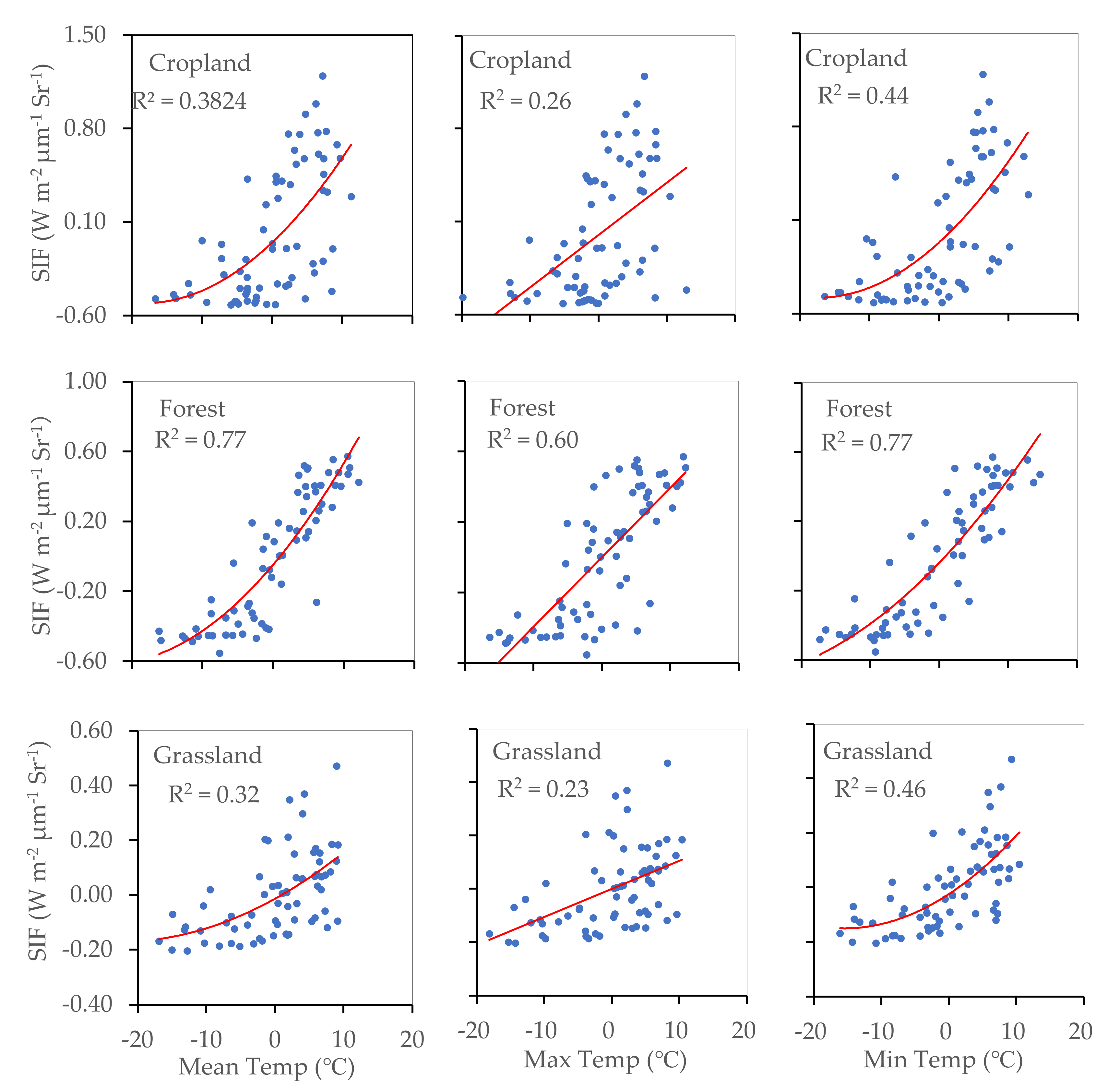
The relationship between SIF and temperature (daily mean temperature, daily maximum temperature, and daily minimum temperature) observed in cropland, forest, and grassland areas is shown in Figure 6. We found that plants were sensitive to temperature, particularly to daily minimum temperature values. SIF showed a closer relationship with temperature in the forest than in the other two land cover types, which may be because the forest region considered in this study was situated at higher latitudes and in a cooler climatic region. In the case of cropland and grassland, the contribution of daily mean temperature to SIF was more than 30%, and the contribution of daily minimum temperature to SIF was more than 40%. This indicated that in cropland and grassland areas, the daily minimum temperature significantly affects the strength of plant photosynthetic processes.
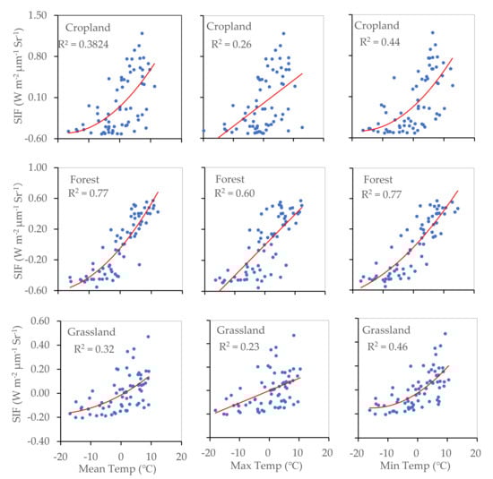
Figure 6.
Relationships between SIF and daily mean temperature, daily maximum temperature, and daily minimum temperature for cropland, forest, and grassland areas (p < 0.001).
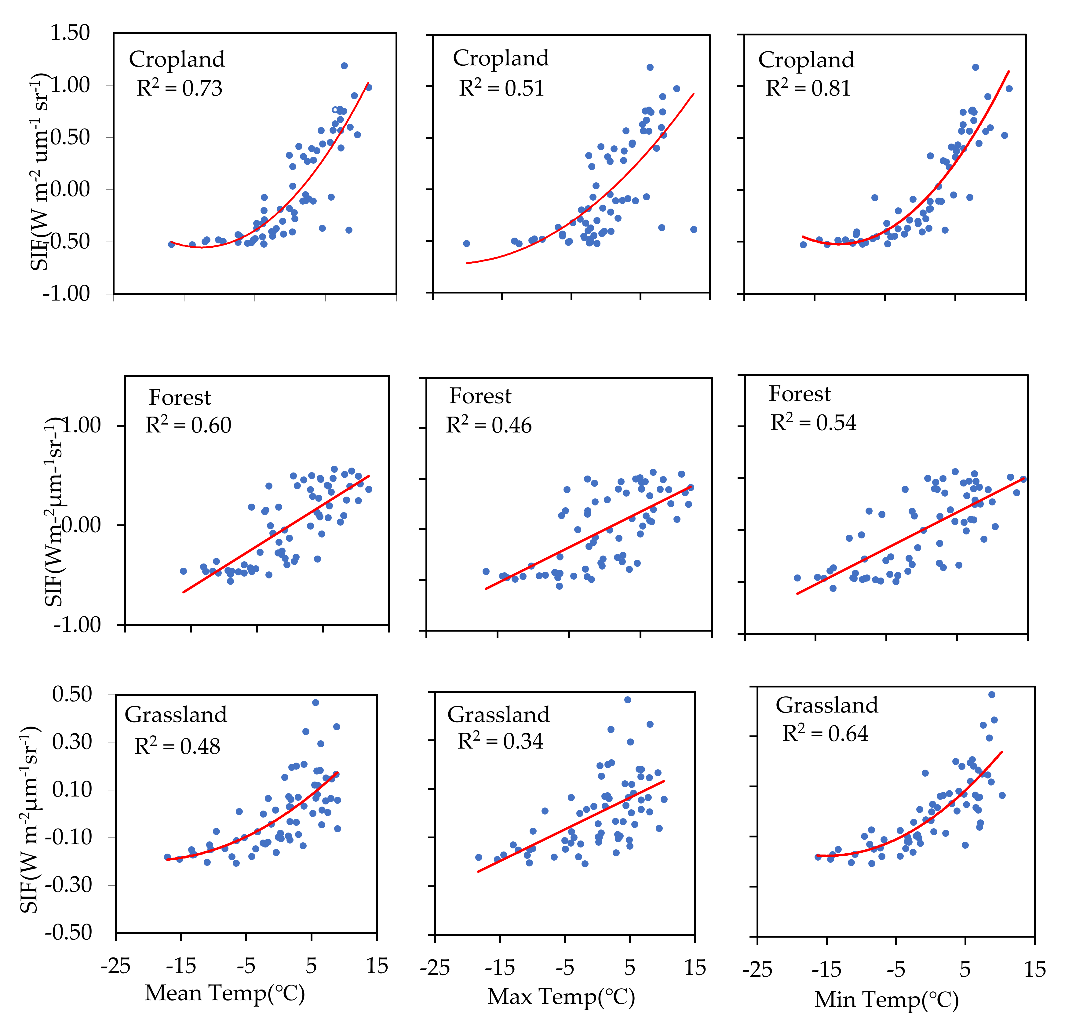
To understand the hysteresis effect of temperature on photosynthesis, we measured the relationship between SIF and the temperature of the previous 16 days (TP16d) (SIF–TP16d) (Figure 7). The correlation coefficient between SIF and TF16d showed a pronounced increase in both cropland and grassland areas compared to temperature recorded in those areas during the same period (T16d). However, the opposite was observed in forested areas. Compared with the previous 16-day mean and maximum temperature values, higher correlation coefficients were found between SIF and the previous 16-day daily minimum temperature for both cropland and grassland.
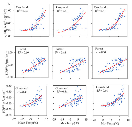
Figure 7.
Relationships between SIF and the previous 16-day daily mean temperature, daily maximum temperature, and daily minimum temperature for cropland, forest, and grassland areas.
No significant correlation was found between SIF and precipitation in either cropland or forest areas, which indicates that precipitation is unlikely to be the limiting factor for crop and tree growth in northeastern China. In the case of grassland, a weak significant correlation was found between SIF and precipitation (R2 = 0.16, p < 0.001), and a slightly higher correlation between SIF and the previous 16-day precipitation (R2 = 0.29, p < 0.001) (not shown here). The grassland area considered in this study is located in the semi-arid region of northeastern China, where the presence or absence of precipitation can have a profound impact on plant growth.
3.5. Accuracy of Modeled SIF at Different Ecosystems
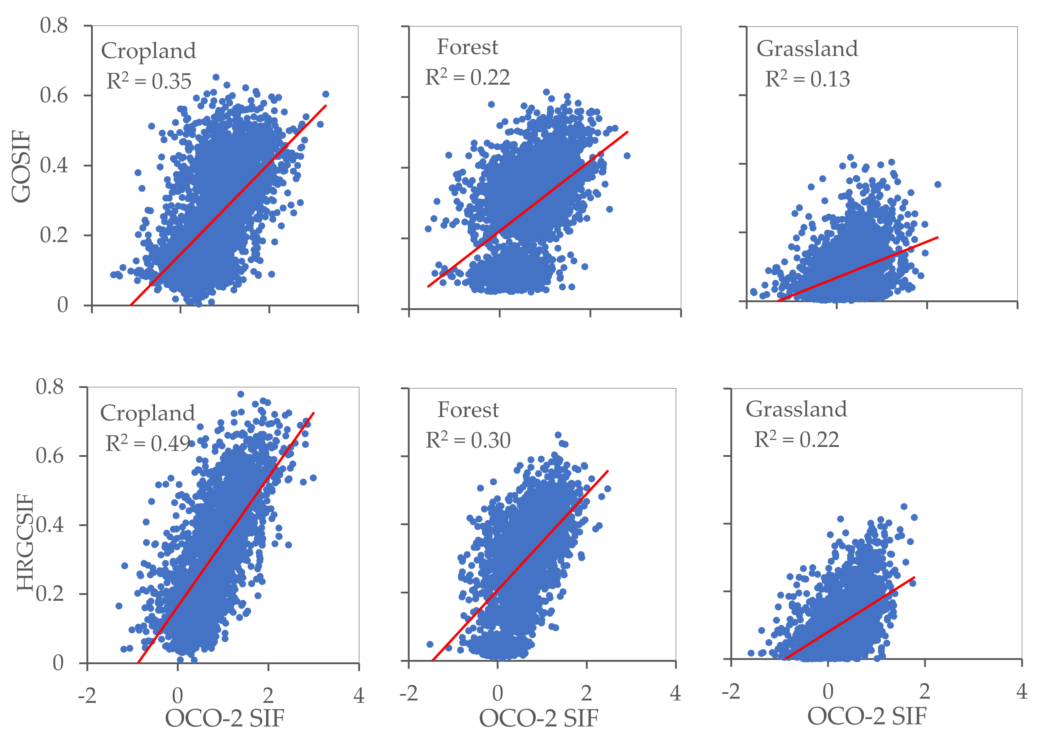
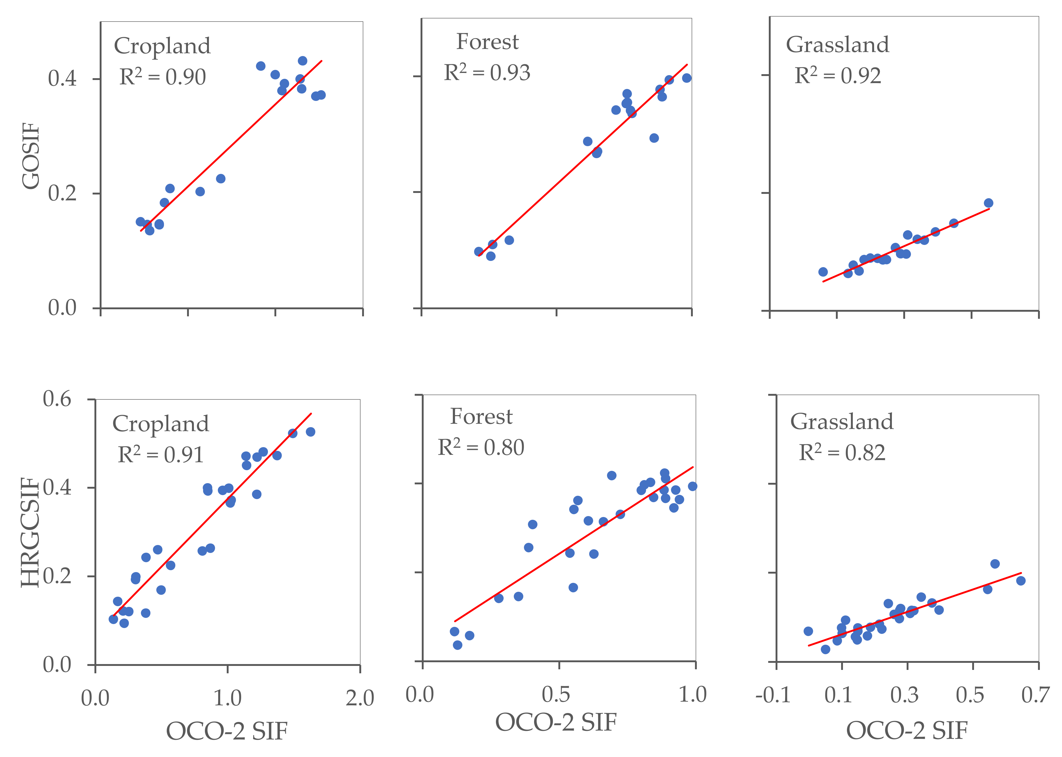
The OCO-2 SIF points as observed values and GOSIF and HRGCSIF as modeled values were utilized to quantify simulation accuracy in different ecosystems. At the footprint scale, we randomly selected 100 OCO-2 points for each ecosystem within the appropriate timeframe and extracted the modelled SIF values. From Figure 8 and Figure 9, it can be observed that R2 values differ between ecosystems at the footprint level. In the case of both GOSIF and HRGCSIF products, the R2 (p < 0.001) values encountered in cropland were higher than those calculated for forest and grassland areas. This pattern was also true for the values of RMSE and slope. At the regional scale, all three ecosystems yielded R2 values higher than 0.8. The value calculated for cropland was particularly high, exceeding 0.9.
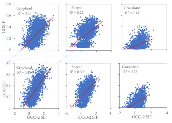
Figure 8.
The accuracy of GOSIF and HRGCSIF for cropland, forest, and grassland at footprint scale (p < 0.001).
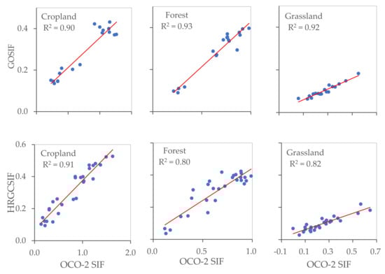
Figure 9.
The accuracy of GOSIF and HRGCSIF for cropland, forest, and grassland at regional scale (p < 0.001).
We can state with some statistical certainty that the comparisons in Figure 8 and Figure 9 support the following claims: (i) Numerical simulations achieved a greater approximation of reality at a regional scale than at the footprint level, with the simulation effect differing among the three ecosystems. Accuracy was highest in cropland, followed by forest, and finally grassland areas; (ii) Simulations under-estimated SIF values at both a regional and at a footprint scale; (iii) Better simulation results can be obtained if we use individual models for each ecosystem.
4. Discussion
4.1. Effect of Spatial Resolutions on the Relationships between SIF and MODIS Products
Scale dependency is an important issue in landscape ecology, and researchers have shown this for several remote sensor-derived parameters, such as land surface temperature and evapotranspiration [43,44,45]. The influencing factors and functions of ecological processes operate differently at varying spatial scales [46]. Scale heterogeneity between SIF and other data products posed great challenges for fully exploring the relationships that might exist between the datasets [16].
At the OCO-2 footprint level, Wood et al. [16], in their study of croplands in the United States, found significant correlations between SIF and EVI (R2 = 0.476, p < 0.001) and also between SIF and FPAR (R2 = 0.490, p < 0.001). Our study obtained a similar but slightly lower correlation coefficient (R2 = 0.39, p < 0.001 and R2 = 0.26, p < 0.001).
From Figure 4 and Figure 5, and Table 2, we found that SIF–EVI, SIF–FPAR, and SIF–LAI have close relationships at a regional scale. However, at the footprint level, the correlations between these variable pairs are weaker. Similar results were produced in our previous research, which showed that with a decrease in spatial resolution, the R2 value of the relationship between SIF and EVI increases [12]. Generally, averaging large areas of vegetation with heterogeneous physiological characteristics increases the SIF–GPP relationship discernable from satellite imagery more so than that at the footprint or leaf level [7,17]. The number of sampling points can also affect the R2 value of regression models. For the regional scale, within 100 samples were used to calculate the relationship between SIF and MODIS indices, and the number for the footprint scale is tens of thousands.
Each ecosystem has a characteristic scale; hence, we must study it at appropriate scales to obtain the right laws and features. Some researchers have argued that ecosystems are highly heterogeneous at spatial scales larger than 5–10 km, and some scholars believe that the characteristic scale of boreal forests is 30 km [12,26,47]. This suggests that it is better to simulate vegetation photosynthesis for different ecosystems using remotely sensed vegetation indices at different scales.
4.2. Effect of Temperature and Precipitation on Plant Photosynthesis
Temperature is one of the most important abiotic factors that regulate plant photosynthesis. Within certain limits, a low temperature decreases the activity of enzymes and the effective rate of carboxylation in the photosynthesis processes, thus affecting the efficiency of photosynthesis [34]. Within the range of plant growth, an increase in temperature will lead to an increase in photosynthesis [48]. However, stresses induced by particularly higher temperatures decrease SIF values through the decrease in red and far-red fluorescence [24,25]. Ren et al. [49] has also argued that in subtropical vegetation, the end of the growing season was positively correlated with the pre-season minimum temperature. However, when the temperature reaches zero degree or lower, plant photosynthesis declines [5,25]. Our results (see Figure 6 and Figure 7) indicate that different plants show different sensitivities to temperature, and that temperatures show a hysteresis effect on plant photosynthesis in cropland and grassland areas, but not in forests. The forested lands considered in this study are mainly distributed at higher latitudes, where temperatures are lower, and temperature is integral for tree growth. However, forests did not appear to be sensitive to the temperatures recorded in the previous 16 days, but rather were more responsive to current mean and minimum temperature levels. Thus, when the growing season starts in a forest, photosynthesis increases and is mainly affected by the current temperature, and is most sensitive to the daily minimum temperature. Higher temperatures can also lead to a decrease in SIF if the temperature exceeds a certain threshold. Lee et al. (2013) found that in Amazonia, when the temperature is lower than 30 °C, SIF and EVI increased with the increase in temperature, and when the temperature was higher than 30 °C, EVI increased, but SIF decreased.
Many researchers have explored how water stress affects vegetation SIF and have found similar conclusions. Lee et al. [4] used Amazonia as the study region and used GOSAT SIF to monitor how seasonal water stress affected plant productivity. They concluded that the drought season easily led to a decline in plant photosynthesis and SIF. Under short-term, mild drought events, plant photosynthesis decreases due to stomatal closure, recovering to its initial level after drought [50]. However, long-term and severe drought will lead to severe photoinhibition and reduced photosynthesis rates [51,52].
The mean annual precipitation of the forest regions considered in this study is approximately 460 mm [12], which is not enough for forest growth. Because of the existence of permafrost in these forest regions, rain that falls to the land surface is fixed by vegetation and cannot infiltrate deep soil [6]. Therefore, we can infer that precipitation is not a factor affecting photosynthesis strength.
For cropland and grassland, the previous 16-day temperature measurement is more sensitive to SIF, which indicates that the cumulative temperature is a more sensitive factor for cropland and grassland areas. Abundant water is an essential prerequisite for cultivation. The croplands located in Songnen Plain (one of China’s most important grain production bases) receive an annual precipitation of 400–600 mm, which is sufficient for crop growth. However, no significant correlation was found between SIF and precipitation in the croplands.
With regard to grassland areas, a significant correlation was found between SIF and current precipitation. A stronger relationship was found between SIF and previous 16-day precipitation. This indicates that precipitation does contribute to SIF in grassland areas, but the contribution is limited, as evidenced by the lower R2 values. The soil in this region is typically grassland zonal soil, which corresponds to climate and vegetation type. Due to limited precipitation, high insolation, and relatively high temperatures, the organic matter content of this soil is limited and this area is prone to desertification and an increased risk of salinization [33]. As a result, photosynthesis strength in the studied grassland area is primarily affected by soil nutrients.
4.3. Simulation Biases in Different Ecosystems
At the footprint scale, the poor correlations detected in the forest areas may be explained by canopy complexity [12,53]. The poor correlations found in the grassland areas may be the result of soil reflectance where the vegetation cover is absent.
Regarding the underestimation of SIF encountered using VIs and meteorological data, we conclude that it is difficult to link stable and structurally driven VIs with the highly variable phenomenon of plant photosynthesis. Another reason is that the reflectance-based VIs typically encounter saturation effects for areas with higher vegetation, such as in forested areas or and in croplands that use higher fertilizers. The VIs are also easily affected by soil reflectance in the grasslands of a semi-arid region [6,12,54].
Many factors lead to the different simulated accuracies for different ecosystems. For different plants in different ecosystems, photosynthesis processes and mechanisms vary. Examples include energy partitioning between photosystems I and II, canopy structure, stoichiometry, and the fluorescence properties of these two photosystems, photorespiration, and photosynthetic pathways (C3 versus C4) [14]. C4 plant photosynthesis evolved from the C3 pathway, adapting to high light intensity, high temperature, and dryness; they have more resource-use efficiencies and photosynthesis strength [22]. Liu et al. [22] also argued that the effect of temperature on SIF for different plants may be affected by other biotic and abiotic factors, and that the relationships observed between SIF and GPP have significant linear relationships for C3 and C4 crops, but have different slope values.
Vegetation canopy structural features, named the clumping index, will significantly affect land surface energy and carbon balances and also vegetation photosynthesis and SIF [7,42,55].
From the analysis above, we can conclude that for different vegetation, photosynthesis processes, and mechanisms, the SIF trend is different because of the difference in canopy structure; hence, it is better to study SIF separately for different ecosystems.
5. Conclusions
This study used OCO-2 SIF data, MODIS products, and meteorological data to explore trends in SIF and the relationship between SIF (and MODIS products) and meteorological variables in three ecosystems (i.e., forest, cropland, and grassland). Our results led us to draw several innovative conclusions:
- (1)
- In different ecosystems, the relationships between the SIF and MODIS products show different correlations. At both a regional and footprint level, EVI demonstrates a close relationship with SIF, indicating that EVI has potential for the simulation of SIF.
- (2)
- With regard to the sensitivity of ecosystems to temperature, forests appear to be more sensitive to daily minimum temperatures, whereas cropland and grassland areas are more sensitive to the former 16 d minimum temperature. In grassland areas, SIF showed a significant correlation with precipitation, although a closer correlation was identified with the former 16-day precipitation. It was concluded that, because of regional differences in meteorological factors, relationships between SIF and meteorological factors are regionally specific.
- (3)
- We took OCO-2 SIF as the observed value to check the accuracy of the simulated SIF products and found different simulation biases for different ecosystems. At the regional scale, R2 values were higher than 0.9 (for GOSIF) and higher than 0.8 (for HRGCSIF). At the footprint scale, the R2 values were different for different ecosystems. We can conclude that SIF must be modeled differently for different ecosystems.
Author Contributions
Methodology, M.G. and J.L. (Jing Li); software, J.L. (Jianuo Li); validation, J.L. (Jianuo Li), C.Z. and F.Z.; formal analysis, M.G. and J.L. (Jing Li); data curation, C.Z. and F.Z.; writing—original draft preparation, M.G.; writing—review and editing, J.L. (Jing Li); visualization, J.L. (Jianuo Li); supervision, J.L. (Jing Li); funding acquisition, M.G. and J.L. (Jing Li). All authors have read and agreed to the published version of the manuscript.
Funding
This research was funded by the National Natural Science Foundation of China (41871103 and 41771179).
Data Availability Statement
Not applicable.
Acknowledgments
We would like to thank the NASA Goddard Earth Science Data and Information Services Center for the use of the OCO-2 data for this study. We would also like to thank the National Meteorological Information Center of China for access to the meteorological data used herein.
Conflicts of Interest
The authors declare no conflict of interest. The funders had no role in the design of the study; in the collection, analyses, or interpretation of data; in the writing of the manuscript, or in the decision to publish the results.
References
- Xue, J.; Su, B. Significant Remote Sensing Vegetation Indices: A Review of Developments and Applications. J. Sens. 2017, 2017, 1353691. [Google Scholar] [CrossRef] [Green Version]
- Gu, X.; Jamshidi, S.; Sun, H.; Niyogi, D. Identifying multivariate controls of soil moisture variations using multiple wavelet coherence in the U.S. Midwest. J. Hydrol. 2021, 602, 126755. [Google Scholar] [CrossRef]
- Jamshidi, S.; Zand-Parsa, S.; Niyogi, D. Assessing Crop Water Stress Index of Citrus Using In-Situ Measurements, Landsat, and Sentinel-2 Data. Int. J. Remote Sens. 2020, 42, 1893–1916. [Google Scholar] [CrossRef]
- Lee, J.-E.; Frankenberg, C.; van der Tol, C.; Berry, J.A.; Guanter, L.; Boyce, C.K.; Fisher, J.; Morrow, E.; Worden, J.R.; Asefi, S.; et al. Forest productivity and water stress in Amazonia: Observations from GOSAT chlorophyll fluorescence. Proc. R. Soc. B Boil. Sci. 2013, 280, 20130171. [Google Scholar] [CrossRef] [PubMed] [Green Version]
- Jonard, F.; De Cannière, S.; Brüggemann, N.; Gentine, P.; Gianotti, D.S.; Lobet, G.; Miralles, D.; Montzka, C.; Pagán, B.; Rascher, U.; et al. Value of sun-induced chlorophyll fluorescence for quantifying hydrological states and fluxes: Current status and challenges. Agric. For. Meteorol. 2020, 291, 108088. [Google Scholar] [CrossRef]
- Wen, L.; Guo, M.; Yin, S.; Huang, S.; Li, X.; Yu, F. Vegetation Phenology in Permafrost Regions of Northeastern China Based on MODIS and Solar-induced Chlorophyll Fluorescence. Chin. Geogr. Sci. 2021, 31, 459–473. [Google Scholar] [CrossRef]
- Marrs, J.K.; Jones, T.S.; Allen, D.W.; Hutyra, L.R. Instrumentation sensitivities for tower-based solar-induced fluorescence measurements. Remote Sens. Environ. 2021, 259, 112413. [Google Scholar] [CrossRef]
- Guo, M.; Li, J.; Yu, F.; Yin, S.; Huang, S.; Wen, L. Estimation of post-fire vegetation recovery in boreal forests using solar-induced chlorophyll fluorescence (SIF) data. Int. J. Wildland Fire 2021, 30, 365. [Google Scholar] [CrossRef]
- Xiao, J.; Chevallier, F.; Gomez, C.; Guanter, L.; Hicke, J.A.; Huete, A.R.; Ichii, K.; Ni, W.; Pang, Y.; Rahman, A.F.; et al. Remote sensing of the terrestrial carbon cycle: A review of advances over 50 years. Remote Sens. Environ. 2019, 233, 111383. [Google Scholar] [CrossRef]
- Hilker, T.; Coops, N.; Wulder, M.; Black, T.A.; Guy, R.D. The use of remote sensing in light use efficiency based models of gross primary production: A review of current status and future requirements. Sci. Total Environ. 2008, 404, 411–423. [Google Scholar] [CrossRef] [Green Version]
- Frankenberg, C.; Butz, A.; Toon, G.C. Disentangling chlorophyll fluorescence from atmospheric scattering effects in O2A-band spectra of reflected sun-light. Geophys. Res. Lett. 2011, 38, L03801. [Google Scholar] [CrossRef]
- Guo, M.; Li, J.; Huang, S.; Wen, L. Feasibility of Using MODIS Products to Simulate Sun-Induced Chlorophyll Fluorescence (SIF) in Boreal Forests. Remote Sens. 2020, 12, 680. [Google Scholar] [CrossRef] [Green Version]
- Helm, L.T.; Shi, H.; Lerdau, M.T.; Yang, X. Solar-induced chlorophyll fluorescence and short-term photosynthetic response to drought. Ecol. Appl. 2020, 30, e02101. [Google Scholar] [CrossRef]
- Sun, Y.; Frankenberg, C.; Wood, J.D.; Schimel, D.S.; Jung, M.; Guanter, L.; Drewry, D.T.; Verma, M.; Porcar-Castell, A.; Griffis, T.J.; et al. OCO-2 advances photosynthesis observation from space via solar-induced chlorophyll fluorescence. Science 2017, 358, eaam5747. [Google Scholar] [CrossRef] [PubMed] [Green Version]
- Zhang, Y.; Guanter, L.; Berry, J.A.; van der Tol, C.; Yang, X.; Tang, J.; Zhang, F. Model-based analysis of the relationship between sun-induced chlorophyll fluorescence and gross primary production for remote sensing applications. Remote Sens. Environ. 2016, 187, 145–155. [Google Scholar] [CrossRef] [Green Version]
- Wood, J.D.; Griffis, T.J.; Baker, J.M.; Frankenberg, C.; Verma, M.; Yuen, K. Multiscale analyses of solar-induced florescence and gross primary production. Geophys. Res. Lett. 2017, 44, 533–541. [Google Scholar] [CrossRef]
- Gu, L.; Han, J.; Wood, J.D.; Chang, C.Y.; Sun, Y. Sun-induced Chl fluorescence and its importance for biophysical modeling of photosynthesis based on light reactions. New Phytol. 2019, 223, 1179–1191. [Google Scholar] [CrossRef] [Green Version]
- Kim, J.; Ryu, Y.; Dechant, B.; Lee, H.; Kim, H.S.; Kornfeld, A.; Berry, J.A. Solar-induced chlorophyll fluorescence is non-linearly related to canopy photosynthesis in a temperate evergreen needleleaf forest during the fall transition. Remote Sens. Environ. 2021, 258, 112362. [Google Scholar] [CrossRef]
- Dechant, B.; Ryu, Y.; Badgley, G.; Zeng, Y.; Berry, J.A.; Zhang, Y.; Goulas, Y.; Li, Z.; Zhang, Q.; Kang, M.; et al. Canopy structure explains the relationship between photosynthesis and sun-induced chlorophyll fluorescence in crops. Remote Sens. Environ. 2020, 241, 111733. [Google Scholar] [CrossRef] [Green Version]
- Mohammed, G.H.; Colombo, R.; Middleton, E.M.; Rascher, U.; van der Tol, C.; Nedbal, L.; Goulas, Y.; Pérez-Priego, O.; Damm, A.; Meroni, M.; et al. Remote sensing of solar-induced chlorophyll fluorescence (SIF) in vegetation: 50 years of progress. Remote Sens. Environ. 2019, 231, 111177. [Google Scholar] [CrossRef]
- Zarco-Tejada, P.; Morales, A.; Testi, L.; Villalobos, F. Spatio-temporal patterns of chlorophyll fluorescence and physiological and structural indices acquired from hyperspectral imagery as compared with carbon fluxes measured with eddy covariance. Remote Sens. Environ. 2013, 133, 102–115. [Google Scholar] [CrossRef]
- Liu, L.; Guan, L.; Liu, X. Directly estimating diurnal changes in GPP for C3 and C4 crops using far-red sun-induced chlorophyll fluorescence. Agric. For. Meteorol. 2017, 232, 1–9. [Google Scholar] [CrossRef]
- Joiner, J.; Yoshida, Y.; Vasilkov, A.; Schaefer, K.; Jung, M.; Guanter, L.; Zhang, Y.; Garrity, S.; Middleton, E.; Huemmrich, K.; et al. The seasonal cycle of satellite chlorophyll fluorescence observations and its relationship to vegetation phenology and ecosystem atmosphere carbon exchange. Remote Sens. Environ. 2014, 152, 375–391. [Google Scholar] [CrossRef] [Green Version]
- Kimm, H.; Guan, K.; Burroughs, C.H.; Peng, B.; Ainsworth, E.A.; Bernacchi, C.J.; Moore, C.E.; Kumagai, E.; Yang, X.; Berry, J.A.; et al. Quantifying high-temperature stress on soybean canopy photosynthesis: The unique role of sun-induced chlorophyll fluorescence. Glob. Chang. Biol. 2021, 27, 2403–2415. [Google Scholar] [CrossRef] [PubMed]
- Ac, A.; Malenovský, Z.; Olejníčková, J.; Gallé, A.; Rascher, U.; Mohammed, G. Meta-analysis assessing potential of steady-state chlorophyll fluorescence for remote sensing detection of plant water, temperature and nitrogen stress. Remote Sens. Environ. 2015, 168, 420–436. [Google Scholar] [CrossRef] [Green Version]
- Li, X.; Xiao, J. A Global, 0.05-Degree Product of Solar-Induced Chlorophyll Fluorescence Derived from OCO-2, MODIS, and Reanalysis Data. Remote Sens. 2019, 11, 517. [Google Scholar] [CrossRef] [Green Version]
- Li, X.; Xiao, J. Mapping Photosynthesis Solely from Solar-Induced Chlorophyll Fluorescence: A Global, Fine-Resolution Dataset of Gross Primary Production Derived from OCO-2. Remote Sens. 2019, 11, 2563. [Google Scholar] [CrossRef] [Green Version]
- Zhang, Y.; Joiner, J.; Alemohammad, S.H.; Zhou, S.; Gentine, P. A global spatially contiguous solar-induced fluorescence (CSIF) dataset using neural networks. Biogeosciences 2018, 15, 5779–5800. [Google Scholar] [CrossRef] [Green Version]
- Yu, L.; Wen, J.; Chang, C.Y.; Frankenberg, C.; Sun, Y. High-Resolution Global Contiguous SIF of OCO-2. Geophys. Res. Lett. 2019, 46, 1449–1458. [Google Scholar] [CrossRef]
- Zhang, X.; Liu, L.; Chen, X.; Gao, Y.; Xie, S.; Mi, J. GLC_FCS30: Global land-cover product with fine classification system at 30 m using time-series Landsat imagery. Earth Syst. Sci. Data 2021, 13, 2753–2776. [Google Scholar] [CrossRef]
- Xu, H. Da Hinggan Ling Mountains Forests in China; Science Press: Beijing, China, 1998; p. 231. [Google Scholar]
- Zhou, Y. Vegetation in Da Kinggan Ling Mountains; Science Press: Beijing, China, 1991. [Google Scholar]
- Han, W.; Hou, X. Climate Change and Grassland Ecosystem—Based on the Field Survey in region of China-Mongolia Typical Grassland; China Agricultural Science and Technology Press: Beijing, China, 2017; p. 158. [Google Scholar]
- Li, X.; Xiao, J.; He, B.; Arain, M.A.; Beringer, J.; Desai, A.R.; Emmel, C.; Hollinger, D.Y.; Krasnova, A.; Mammarella, I.; et al. Solar-induced chlorophyll fluorescence is strongly correlated with terrestrial photosynthesis for a wide variety of biomes: First global analysis based on OCO-2 and flux tower observations. Glob. Chang. Biol. 2018, 24, 3990–4008. [Google Scholar] [CrossRef] [PubMed]
- Frankenberg, C.; O‘Dell, C.; Berry, J.; Guanter, L.; Joiner, J.; Köhler, P.; Pollock, R.; Taylor, T.E. Prospects for chlorophyll fluorescence remote sensing from the Orbiting Carbon Observatory-2. Remote Sens. Environ. 2014, 147, 1–12. [Google Scholar] [CrossRef] [Green Version]
- Li, X.; Xiao, J.; He, B. Chlorophyll fluorescence observed by OCO-2 is strongly related to gross primary productivity estimated from flux towers in temperate forests. Remote Sens. Environ. 2018, 204, 659–671. [Google Scholar] [CrossRef]
- Myneni, R.; Knyazikhin, Y.; Park, T. MOD15A2H MODIS Leaf Area Index/FPAR 8-Day L4 Global 500m SIN Grid V006. NASA EOSDIS Land Processes DAAC. LP DAAC, Terra. 2015; Volume 6. Available online: https://modis.gsfc.nasa.gov/data/dataprod/mod15.php (accessed on 19 January 2022).
- Yu, L.; Wen, J.; Chang, C.Y.; Frankenberg, C.; Sun, Y. High Resolution Global Contiguous SIF Estimates Derived from OCO-2 SIF and MODIS; Version 2; ORNL DAAC: Oak Ridge, TN, USA, 2019. [Google Scholar] [CrossRef]
- Guo, M.; Li, J.; He, H.S.; Xu, J.; Jin, Y. Detecting Global Vegetation Changes Using Mann-Kendal (MK) Trend Test for 1982–2015 Time Period. Chin. Geogr. Sci. 2018, 28, 907–919. [Google Scholar] [CrossRef] [Green Version]
- Sarvia, F.; De Petris, S.; Borgogno-Mondino, E. Exploring Climate Change Effects on Vegetation Phenology by MOD13Q1 Data: The Piemonte Region Case Study in the Period 2001–2019. Agronomy 2021, 11, 555. [Google Scholar] [CrossRef]
- Turner, A.J.; Köhler, P.; Magney, T.S.; Frankenberg, C.; Fung, I.; Cohen, R.C. A double peak in the seasonality of California‘s photosynthesis as observed from space. Biogeosciences 2020, 17, 405–422. [Google Scholar] [CrossRef] [Green Version]
- Braghiere, R.K.; Wang, Y.; Doughty, R.; Sousa, D.; Magney, T.; Widlowski, J.-L.; Longo, M.; Bloom, A.A.; Worden, J.; Gentine, P.; et al. Accounting for canopy structure improves hyperspectral radiative transfer and sun-induced chlorophyll fluorescence representations in a new generation Earth System model. Remote Sens. Environ. 2021, 261, 112497. [Google Scholar] [CrossRef]
- Bartkowiak, P.; Castelli, M.; Notarnicola, C. Downscaling Land Surface Temperature from MODIS Dataset with Random Forest Approach over Alpine Vegetated Areas. Remote Sens. 2019, 11, 1319. [Google Scholar] [CrossRef] [Green Version]
- Jamshidi, S.; Zand-Parsa, S.; Jahromi, M.N.; Niyogi, D. Application of A Simple Landsat-MODIS Fusion Model to Estimate Evapotranspiration over A Heterogeneous Sparse Vegetation Region. Remote Sens. 2019, 11, 741. [Google Scholar] [CrossRef] [Green Version]
- Jamshidi, S.; Zand-Parsa, S.; Pakparvar, M.; Niyogi, D. Evaluation of Evapotranspiration over a Semiarid Region Using Multiresolution Data Sources. J. Hydrometeorol. 2019, 20, 947–964. [Google Scholar] [CrossRef]
- Forman, R.T.T.; Godron, M. Landscape Ecology; John Wiley & Sons, Inc.: Hoboken, NJ, USA, 1986. [Google Scholar]
- Duveiller, G.; Cescatti, A. Spatially downscaling sun-induced chlorophyll fluorescence leads to an improved temporal correlation with gross primary productivity. Remote Sens. Environ. 2016, 182, 72–89. [Google Scholar] [CrossRef]
- Hikosaka, K.; Ishikawa, K.; Borjigidai, A.; Muller, O.; Onoda, Y. Temperature acclimation of photosynthesis: Mechanisms involved in the changes in temperature dependence of photosynthetic rate. J. Exp. Bot. 2005, 57, 291–302. [Google Scholar] [CrossRef] [PubMed] [Green Version]
- Ren, P.; Liu, Z.; Zhou, X.; Peng, C.; Xiao, J.; Wang, S.; Li, X.; Li, P. Strong controls of daily minimum temperature on the autumn photosynthetic phenology of subtropical vegetation in China. For. Ecosyst. 2021, 8, 31. [Google Scholar] [CrossRef]
- Miyashita, K.; Tanakamaru, S.; Maitani, T.; Kimura, K. Recovery responses of photosynthesis, transpiration, and stomatal conductance in kidney bean following drought stress. Environ. Exp. Bot. 2005, 53, 205–214. [Google Scholar] [CrossRef]
- Yu, S.; Zhang, N.; Kaiser, E.; Li, G.; An, D.; Sun, Q.; Chen, W.; Liu, W.; Luo, W. Integrating chlorophyll fluorescence parameters into a crop model improves growth prediction under severe drought. Agric. For. Meteorol. 2021, 303, 108367. [Google Scholar] [CrossRef]
- Chaves, M.M.; Flexas, J.; Pinheiro, C. Photosynthesis under drought and salt stress: Regulation mechanisms from whole plant to cell. Ann. Bot. 2009, 103, 551–560. [Google Scholar] [CrossRef] [PubMed] [Green Version]
- Zhang, Z.; Wang, S.; Qiu, B.; Song, L.; Zhang, Y. Retrieval of sun-induced chlorophyll fluorescence and advancements in carbon cycle application. Yaogan Xuebao/J. Remote. Sens. 2019, 23, 37–52. [Google Scholar] [CrossRef]
- Guanter, L.; Zhang, Y.; Jung, M.; Joiner, J.; Voigt, M.; Berry, J.A.; Frankenberg, C.; Huete, A.R.; Zarco-Tejada, P.; Lee, J.-E.; et al. Global and time-resolved monitoring of crop photosynthesis with chlorophyll fluorescence. Proc. Natl. Acad. Sci. USA 2014, 111, E1327–E1333. [Google Scholar] [CrossRef] [Green Version]
- Sun, Q.; Jiao, Q.; Liu, L.; Liu, X.; Qian, X.; Zhang, X.; Zhang, B. Improving the Retrieval of Forest Canopy Chlorophyll Content From MERIS Dataset by Introducing the Vegetation Clumping Index. IEEE J. Sel. Top. Appl. Earth Obs. Remote Sens. 2021, 14, 5515–5528. [Google Scholar] [CrossRef]

Publisher’s Note: MDPI stays neutral with regard to jurisdictional claims in published maps and institutional affiliations. |
© 2022 by the authors. Licensee MDPI, Basel, Switzerland. This article is an open access article distributed under the terms and conditions of the Creative Commons Attribution (CC BY) license (https://creativecommons.org/licenses/by/4.0/).