Technical Note

MCMC Method of Inverse Problems Using a Neural Network—Application in GPR Crosshole Full Waveform Inversion: A Numerical Simulation Study

1
College of Geo-Exploration Science and Technology, Jilin University, Changchun 130026, China
2
College of Instrumentation & Electrical Engineering, Jilin University, Changchun 130026, China
*
Author to whom correspondence should be addressed.
Remote Sens. 2022, 14(6), 1320; https://doi.org/10.3390/rs14061320
Submission received: 24 January 2022 / Revised: 3 March 2022 / Accepted: 6 March 2022 / Published: 9 March 2022

Abstract

:
Ground-penetrating radar (GPR) crosshole tomography is widely applied to subsurface media images. However, the inadequacies of ray methods may limit the resolution of crosshole radar images, since the ray method is a type of high-frequency approximation. To solve this problem, the full waveform method is introduced for GPR inversion. However, full waveform inversion is computationally expensive. In this paper, we introduce a trained neural network that can be evaluated very quickly to replace a computationally intensive forward model. Additionally, the forward error of the trained neural network can be statistically analyzed. We demonstrate a methodology for a full waveform inversion of crosshole ground-penetrating radar data using the Markov chain Monte Carlo (MCMC) method. An accurate forward model based on Maxwell’s equations is replaced by a quickly trained neural network. This method achieves a high computation efficiency, which is four orders of magnitude faster than the accurate forward model. The inversion result of the synthetic waveform data shows a good performance of the trained neural network, which greatly improves the calculation efficiency.

1. Introduction

Ground-penetrating radar (GPR) crosshole tomography is widely used to map subsurface electrical properties, e.g., electrical conductivity and dielectric permittivity, which are important in investigating environments [1,2,3,4]. A GPR crosshole experiment includes transmitting radar antennas and receiving antennas that are distributed in the opposite borehole. Transmitting antennas (20 MHz to 1 GHz) generate high-frequency electromagnetic energy to acquire crosshole radar data.
Inversion refers to using physical phenomena observed on the earth’s surface to infer the spatial changes of the physical structure of the underground medium. To solve the inversion problem, a number of inversion methods have evolved over the past two decades, including deterministic inversion algorithms and probabilistic inversion [5]. Compared with deterministic inversion algorithms [6,7,8], probabilistic inversion methods do not need an accurate a priori model and can use any a priori known information, regardless of its complexity. The result of the probabilistic inversion is the a posteriori probability density [9]. The model variability of posterior samples can reflect the information contained in the posterior probability density, which can solve more sophisticated questions [10]. To solve the highly nonlinear inversion problem, Mosegaard et al. proposed the extended Metropolis algorithm to sample the a posteriori probability density [11]. Instead of an explicit mathematical expression of a priori information, the extended Metropolis algorithm only needs a “black box” algorithm to sample the a priori probability. A sequential Gibbs sampler is proposed to serve as a black box algorithm to sample a priori information defined by any geostatistical algorithm [12,13]. In this way, sampling the a posteriori probability density becomes very flexible [14,15,16,17].
Ray tomographic methods are generally based on ray theory, which uses only a small portion of signal information, limiting the resolution of crosshole radar images [18,19]. To solve this problem, a full waveform method is introduced for GPR inversion. Ernst successfully used full waveform data from a GPR crosshole to invert electrical conductivity and dielectric permittivity [20]. Klotzsche et al. characterized a gravel aquifer by the full waveform crosshole ground-penetrating radar data [21]. Cordua obtained the first a posteriori probability density of full waveform GPR crosshole data [22]. Hansen implemented an efficient Monte Carlo sampling method using a neural network to simulate travel time to replace the ray methods [23]. However, the problem of the huge computational costs of full waveform inversion has not been solved.
In this paper, to obtain fast full waveform inversion, we introduce the trained neural network forward model into the MCMC method of GPR crosshole data. The inverse problem refers to obtaining dielectric permittivity through full waveform GPR crosshole data. We replace a numerical complex forward model based on the 2D FDTD solution of Maxwell’s equations with a two-layer feedforward network. Taking advantage of the fast mapping of a two-layer feedforward network, this MCMC inverts four orders of magnitude faster than the 2D FDTD solution of Maxwell’s equations.
This paper is organized as follows: First, we introduce probability inversion using the MCMC method, including its theories and formulas. Second, we present the forward method based on the 2D FDTD solution of Maxwell’s equations. Then, we briefly introduce the two-layer feedforward network. Finally, we use the synthetic FWI data from a ground-penetrating radar crosshole to analyze the error and efficiency of the trained neural network.

2. Methods

2.1. Probabilistically Formulated Inversion

For geophysical inverse problems, the subsurface can be described by a set of parameters m , and the observed data can be represented by a dataset d . Hence, the forward relation between m and d is as follows [5]:
d = f m
where the function f is a mapping operator solved by a physical relation. The corresponding inverse problem can be expressed as follows:
m = f 1 d
In this formula, the inverse operator f 1 is difficult to obtain because it is non-trivial or does not exist. Furthermore, the forward relation is an approximation to the correct physical law. In this paper, relative dielectric permittivity refers to the subsurface parameters m that we want to invert, and the observed data are the waveform data of the GPR crosshole.
For probabilistic inversion, the corresponding inversion formula is as follows [5]:
σ M m = k ρ M m L m
where ρ M m is the a priori probability density, which represents the a priori information of the model parameters. The solution of the inverse problem is the a posteriori probability distribution σ M m . k is a normalization factor, and L m is the likelihood function. L m is a probabilistic measure that describes how well the modeled data explain the observed data. Its general formula is given by the following:
L m = d d ρ D g m θ d | m μ D d
where ρ D g m represents measurement uncertainties that are mainly related to the recording instrument. θ ( d | m ) represents the model error caused by the imperfect forward method defective parameterization. μ D d describes the homogeneous state of information, which ensures parameterization is invariant when the coordinate system changes. In most cases, μ D d can be assumed to be constant.

2.2. Extended Metropolis Algorithm

For non-linear and non-Gaussian problems, obtaining the mathematical formula of the a priori probability density is difficult. The extended Metropolis algorithm can solve this difficulty using sequential Gibbs sampling to directly sample ρ M m . To perform the extended Metropolis algorithm, we used a sequential Gibbs sampler as a part of the extended Metropolis algorithm to directly sample ρ M m . The extended Metropolis algorithm is performed as follows [14]:
  • Start in the current model, m cur , which constitutes the a priori probability density. Using the sequential Gibbs sampler to sample m cur , a new model candidate m pro is generated.
  • Calculate the probability of accepting the proposed model using the ratio of likelihood function: P a c c = m i n ( 1 , L m pro L m cur )
  • If m pro is accepted, use m pro instead of m cur . Consequently, the proposed model takes the place of the current model: m cur = m pro . Otherwise, the random walker staying at a location in m cur and m cur is counted again.

2.3. Forward Model Based on Waveform

For the forward model, several methods can be selected to simulate the GPR signal’s wavefield. In this paper, we chose the 2D FDTD solution of Maxwell’s equations in transverse electric mode. This FDTD method simulates the vertical component of the electrical field as the observed data. For electromagnetic wave propagation, the transverse electric or TE modes of Maxwell’s equations in the (x, z) plane of Cartesian coordinates are as follows [24]:
E x t = 1 ε H y z σ E x
E z t = 1 ε H y x σ E x
H y t = 1 μ E z x E x z
where E x and E z represent the horizontal and vertical components of the electric field, respectively; ε is the dielectric permittivity; σ is the electrical conductivity; H y is the magnetic field perpendicular to the propagation plane; and μ represents the magnetic permeability, which is equivalent to the free-space permeability assumed to be constant in the following.
We used the FDTD techniques [24,25] based on the staggered grid finite difference operator with second-order accuracy in space and time to solve Equations (5)–(7). A generalized perfectly matched layer (GPML) surrounding the edges of the FDTD grid absorbs the artificial reflections at the edges of the model space. Near the surface, electromagnetic signals are mainly affected by dielectric permittivity and electrical conductivity. Permittivity primarily controls the phases, and conductivity primarily controls the amplitudes of the observed signals. In this paper, we consider only the influence of the dielectric permittivity. For all examples presented in this paper, we inverted the permittivity while keeping the conductivities fixed [8].

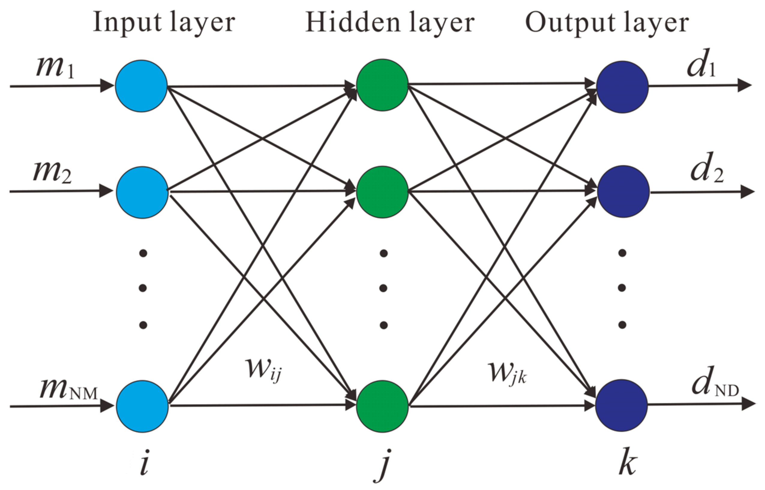
2.4. Solving the forward Problem Using a Trained Neural Network

Trained neural networks are methods that infer a non-linear mapping operator from one data set to another data set. For the inversion problem, neural networks can be applied to simulate the forward operator and the inverse operator [26,27,28,29]. In this paper, we used neural networks to replace the computationally expensive forward model in Equations (5)–(7). The neural networks can evaluate the forward problem quickly. However, this also leads to some modeling errors. We used a Gaussian probability distribution to quantify the modeling error θ ( d | m ) caused by the trained neural network. In this paper, we used a two-layer feedforward neural network containing a hidden layer [30]. It should be noted that we can use any regression-type network. The main reason we chose the two-layer feedforward network is that, once trained, the mapping of the network on a new model is potentially very fast and meets our requirement for efficiency. The mathematical expression of this network is as follows:
d k = h 1 j NH w j k 2 h 2 i NM w i j 1 m i
d k = d 1 , d 2 , , d ND represents each of the observed data d , and ND is the number of observed data parameters. m i = m 1 , m 2 , , m ND represents each of the model parameters. NM represents the number of parameters in the model.
NH represents the number of hidden layers. h 1 and h 2 are two sigmoidal types of activation functions. w i j 1 refers to the weights of the units in the first layer, and w j k 2 refers to the weights of the units in the second layer. If we have a sufficient training set and enough units of the hidden layer, we can replace any continuous mapping. Figure 1 shows the one hidden-layer network architecture that we used.
For probabilistically formulated inverse problems, a great quantity of training data can be easily generated from the a priori distribution ρ M m . The accuracy of the network is highly dependent on the size of the training data set NT. We can create an arbitrarily large sample of the a priori M and simulate the observational data D using the forward model. If we want to train the network needs NT times, the M and D should consist of NT samples.
For all models in M, the corresponding simulated observational data are simulated by the exact, but expensive, forward model based on the FDTD solution of Maxwell’s equations, f FWI . The neural network training result, f nn , provides an approximation of f FWI . In other words, using f nn leads to a modeling error. To evaluate the training effect, we need the model error. To estimate the forward model error between f FWI and f nn , we can analyze Nr samples from the a priori model.
First, we use the a priori distribution to generate Nr realizations in M * = m 1 , m 2 , , m Nr . We use both f FWI and f nn to compute the observed data set D FWI and D nn of every model in M * . Second, we obtain a sample of the modeling error θ ( d | m ) using D θ   =   D FWI     D nn and use the method of Hansen et al. to obtain a Gaussian model of modeling error [31].

3. Experimental Validation

For the synthetic example, we simulated a reference model m of size 5.2 × 12 m (26 × 60 = 1560 pixels of size 0.2 m × 0.2 m). This model is created by a multivariate Gaussian probability distribution, with the mean of the relative dielectric permittivity ε r being 4.0 and the variance being 0.75. In this reference model, the electrical conductivity is assumed to be a constant value of 3 mS/m. There is a relatively high dielectric permittivity structure located at a depth of about 4 m, which is the main feature of our inversion.
To obtain the observed data, we designed a recording geometry of the ground-penetrating radar (GPR) cross borehole. Figure 2 shows a recording geometry that contains four transmitters, and each borehole contains two (the transmitters are represented by red crosses, one at 3 m and one at 9 m). The receivers are represented by black dots at equally spaced intervals of 1.5 m in the two boreholes. Due to the effects of wave guiding [32], the travel path is not at the center of the antenna, but at the tips of the antenna [33]. Data where the angle between a transmitter–receiver and the horizontal is larger than 45° are omitted. This decision was made with a similar reasoning to the parameters inferred in Cordua using the same geometrical setup [22].
The FDTD algorithm is used to calculate a full waveform synthetic dataset. The FDTD model for solving Maxwell’s equations uses a regular grid consisting of square elements of 0.1 m × 0.1 m, and the number of boundary elements is 40. In the synthetic data, we assumed that the source pulse is known, which was a ricker wavelet, and that the central frequency is 100 MHz. For the field data, it should be noted that the source wavelet needs to be estimated. Some methods can estimate the source wavelet [34,35].
The recorded synthetic observational data are the vertical components of the electrical field. They contain a total of 20 waveform traces. We added Gaussian-distributed data uncertainties to the waveform data. In Figure 3, we present five waveform traces generated by a transmitter at a depth of 3 m in the left borehole. The signal-to-noise ratios from the top are 8, 15, 20, 30, and 40, respectively. The blue dotted curves represent noise-free waveforms, and the red curves represent noisy waveforms. As can be seen in Figure 3, the matching of the waveforms from top to bottom gradually becomes better between the noise-free waveforms and the noisy waveforms.
For this reference model and observed data, we set the size of the input layer NM as 1560. The output layer ND was 460. The number of hidden units NH was 100. The accuracy of the network was very heavily affected by the size of the training data set NT. We generated four training data sets whose training sizes were NT = [1000, 5000, 10,000, 20,000] to analyze the training effect of the neural network. The corresponding four forward models refer to f 1000 , f 5000 , f 10,000 , and f 20,000 . Before the inversion, we needed to obtain NT models as unconditional realizations of the a priori distribution and the observed data computed by the forward model f FWI described previously. Figure 4 shows five different sampling models generated from the a priori probability density.
The extended Metropolis algorithm was used to obtain the a posteriori probability density. Figure 5 shows four groups of inversion results based on the four neural network forward models. The synthetic GPR shows that the trained neural network can obtain the main features of the inverse models, even when using the neural network forward model whose training size is 5000. Clearly, the inversion models contain features that appear to be consistent with those in the reference model. The relatively high dielectric permittivity structures are located at a depth of about 4 m. This proves the effectiveness of the MCMC inversion based on the trained neural network. To test the training effect, we used the observed waveform created by the FDTD method to compare the simulated waveform of the four neural networks. We selected trace 1 and trace 5 of the top left borehole, corresponding to the minimum signal-to-noise ratios trace and the maximum signal-to-noise ratios trace, as Figure 6 shows. There are some obvious distortion points in the simulated waveforms created by f 1000 and f 5000 . The simulated waveforms created by f 20,000 are more similar to the observed waveforms.
To analyze the forward modeling error of the neural network-based forward, we created a 1D distribution of the modeling error, which was created by 6000 realizations, in Figure 7. Clearly, the magnitude of modeling error using the trained neural network decreases as training times increases. Figure 8 shows the covariance model of four forward methods based on the trained neural network. f 1000 leads to a more correlated covariance model compared with f 5000 , f 10,000 , and f 20,000 .
Table 1 lists the computation time of the forward model. We tested the forward model 10,000 times in the extended metropolis algorithm to record the computation time. For the four forward models based on a neural network, the running time of the extended Metropolis algorithms are similar, and all the step sizes tend to be stable after 3000 iterations. Table 1 shows that, compared with the full waveform forward model f FWI , the forward model based on our trained neural network is more than four orders of magnitude faster. This is a significant improvement in computation efficiency.

4. Conclusions

This paper replaces a computationally complex full waveform forward model with a fast forward model based on a trained neural network, which, when combined with the MCMC method, solves the inversion problem. Although the neural network of the minimum training time, 1000, cannot reflect the correct features of the reference model, the neural network whose training size is 5000 contains features that are consistent with the reference model. There are some obvious distortion points in the simulated waveform created by the neural network with less training times. When the training times reach 10,000, the distortion disappears clearly in the simulated waveform. The error analysis shows that the inversion effect becomes better when the size of the training times is increased. Compared with the full waveform forward model based on the 2D FDTD solution of Maxwell’s equations, our trained neural network is more than four orders of magnitude faster. The results demonstrate that trained neural networks can be used to describe a full waveform forward model, which is an obvious advantage in application. In the future, we will research how to apply this method to some complex models and try to apply it to field data.

Author Contributions

Conceptualization, S.W., L.H. and X.H.; methodology, S.W. and X.H.; Code, S.W., X.G. and L.H.; validation, S.W.; formal analysis, S.W. and X.G.; writing—original draft preparation, S.W. and X.G.; writing—review and editing, X.G., S.Z. and P.Z. All authors have read and agreed to the published version of the manuscript.

Funding

This research was funded by the National Natural Science Foundation of China, grant numbers 42130805, 42074151, and 42004106.

Institutional Review Board Statement

Not Applicable.

Informed Consent Statement

Not Applicable.

Data Availability Statement

Not Applicable.

Conflicts of Interest

The authors declare no conflict of interest.

References

  1. Rasol, M.A.; Pérez-Gracia, V.; Solla, M.; Pais, J.C.; Fernandes, F.M.; Santos, C. An experimental and numerical approach to combine Ground Penetrating Radar and computational modeling for the identification of early cracking in cement concrete pavements. NDT E Int. 2020, 115, 102293. [Google Scholar] [CrossRef]
  2. Solla, M.; Lagüela, S.; Riveiro, B.; Lorenzo, H. Non-destructive testing for the analysis of moisture in the masonry arch bridge of Lubians (Spain). Struct. Control. Health Monit. 2013, 20, 1366–1376. [Google Scholar] [CrossRef]
  3. Cui, T.J.; Chew, W.C.; Aydiner, A.A.; Chen, S.Y. Inverse scattering of two-dimensional dielectric objects buried in a lossy earth using the distorted Born iterative method. IEEE Trans. Geosci. Remote Sens. 2001, 39, 339–346. [Google Scholar]
  4. Zhou, H.; Sato, M. Subsurface cavity imaging by crosshole borehole radar measurements. IEEE Trans. Geosci. Remote Sens. 2004, 42, 335–341. [Google Scholar] [CrossRef]
  5. Tarantola, A.; Valette, B. Inverse problems = quest for information. J. Geophys. 1982, 50, 159–170. [Google Scholar]
  6. Holliger, K.; Musil, M.; Maurer, H. Ray-based amplitude tomography for crosshole georadar data: A numerical assessment. J. Appl. Geophys. 2001, 47, 285–298. [Google Scholar] [CrossRef]
  7. Linde, N.; Binley, A.; Tryggvason, A.; Pedersen, L.B.; Revil, A. Improved hydrogeophysical characterization using joint inversion of cross-hole electrical resistance and ground-penetrating radar traveltime data. Water Resour. Res. 2006, 42, W1240. [Google Scholar] [CrossRef] [Green Version]
  8. Meles, G.A.; Van der Kruk, J.; Greenhalgh, S.A.; Ernst, J.R.; Maurer, H.; Green, A.G. A new vector waveform inversion algorithm for simultaneous updating of conductivity and permittivity parameters from combination crosshole/borehole-to-surface GPR data. IEEE Trans. Geosci. Remote Sens. 2010, 48, 3391–3407. [Google Scholar] [CrossRef]
  9. Hansen, T.M.; Journel, A.G.; Tarantola, A.; Mosegaard, K. Linear inverse Gaussian theory and geostatistics. Geophysics 2006, 71, R101–R111. [Google Scholar] [CrossRef]
  10. Mosegaard, K. Resolution analysis of general inverse problems through inverse Monte Carlo sampling. Inverse Probl. 1998, 14, 405–426. [Google Scholar] [CrossRef]
  11. Mosegaard, K.; Tarantola, A. Monte Carlo sampling of solutions to inverse problems. J. Geophys. Res. 1995, 100, 431–447. [Google Scholar] [CrossRef]
  12. Hansen, T.M.; Cordua, K.C.; Mosegaard, K. Inverse problems with non-trivial priors-efficient solution through sequential Gibbs sampling. Comput. Geosci. 2012, 16, 593–611. [Google Scholar] [CrossRef] [Green Version]
  13. Hansen, T.M.; Mosegaard, K.; Cordua, K.S. Using geostatisticsto describe complex a priori information for inverse problems. In Geostatistics; Ortiz, J.M., Emery, X., Eds.; Gecamin Ltd.: Santiago, Chile, 2008; Volume 1. [Google Scholar]
  14. Hansen, T.M.; Cordua, K.S.; Zunino, A.; Mosegaard, K. Probabilistic integration of geo-information. In Integrated Imaging of the Earth: Theory and Applications; Wiley: Hoboken, NJ, USA, 2016; Volume 218, pp. 93–116. [Google Scholar]
  15. Wang, S.; Han, L.; Gong, X.; Zhang, S.; Huang, X.; Zhang, P. Full-Waveform Inversion of Time-Lapse Crosshole GPR Data Using Markov Chain Monte Carlo Method. Remote Sens. 2021, 13, 4530. [Google Scholar] [CrossRef]
  16. Journel, A.; Zhang, T. The necessity of a multiple-point prior model. Math. Geol. 2006, 38, 591–610. [Google Scholar] [CrossRef]
  17. Moghadas, D.; Vrugt, J.A. The influence of geostatistical prior modeling on the solution of DCT-based Bayesian inversion: A case study from Chicken Creek catchment. Remote Sens. 2019, 11, 1549. [Google Scholar] [CrossRef] [Green Version]
  18. Balkaya, C.; Akcıg, Z.; Gokturkler, G. A comparison of two travel-time tomography schemes for crosshole radar data: Eikonal-equation-based inversion versus ray-based inversion. J. Environ. Eng. Geophys. 2010, 15, 203–218. [Google Scholar] [CrossRef]
  19. Qin, H.; Wang, Z.; Tang, Y.; Geng, T. Analysis of Forward Model, Data Type, and Prior Information in Probabilistic Inversion of Crosshole GPR Data. Remote Sens. 2021, 13, 215. [Google Scholar] [CrossRef]
  20. Ernst, J.R.; Maurer, H.; Green, A.G.; Holliger, K. Full-waveform inversion of crosshole radar data based on 2-D finite-difference time-domain solutions of Maxwell’s equations. IEEE Trans. Geosci. Remote Sens. 2007, 45, 2807–2828. [Google Scholar] [CrossRef]
  21. Klotzsche, A.; van der Kruk, J.; Meles, G.A.; Doetsch, J.A.; Maurer, H.; Linde, N. Full-waveform inversion of cross-hole ground-penetrating radar data to characterize a gravel aquifer close to the Thur River, Switzerland. Near Surf. Geophys. 2010, 8, 635–649. [Google Scholar] [CrossRef]
  22. Cordua, K.S.; Hansen, T.M.; Mosegaard, K. Monte Carlo full-waveform inversion of crosshole GPR data using multiple-point geostatistical a priori information. Geophysics 2012, 77, H19–H31. [Google Scholar] [CrossRef] [Green Version]
  23. Hansen, T.; Cordua, K. Efficient Monte Carlo sampling of inverse problems using a neural network-based forward—Applied to GPR crosshole traveltime inversion. Geophys. J. Int. 2017, 211, 1524–1533. [Google Scholar] [CrossRef]
  24. Taflove, A.; Hagness, S.C. Computational Electrodynamics the Finite-Difference Time-Domain Method, 2nd ed.; Artech House: Boston, MA, USA, 2000. [Google Scholar]
  25. Yee, K.S. Numerical solution of initial boundary value problems involving Maxwell’s equations in isotropic media. IEEE Trans. Antennas Propag. 1966, 14, 302–307. [Google Scholar]
  26. Singh, U.K.; Tiwari, R.; Singh, S. Neural network modeling and prediction of resistivity structures using VES Schlumberger data over a geothermal area. Comput. Geosci. 2013, 52, 246–257. [Google Scholar] [CrossRef]
  27. Li, G.; You, J.; Liu, X. Support vector machine (SVM) based prestack avo inversion and its applications. J. Appl. Geophys. 2015, 120, 60–68. [Google Scholar] [CrossRef]
  28. Poulton, M.M. Computational Neural Networks for Geophysical Data Processing; Elsevier: Amsterdam, The Netherlands, 2001; Volume 30. [Google Scholar]
  29. Krasnopolsky, V.M.; Schiller, H. Some neural network applications in environmental sciences. Part I: Forward and inverse problems in geophysical remote measurements. Neural Netw. 2003, 16, 321–334. [Google Scholar] [CrossRef]
  30. Bishop, C.M. Neural Networks for Pattern Recognition; Oxford University Press: Oxford, UK, 1995. [Google Scholar]
  31. Hansen, T.M.; Cordua, K.S.; Jacobsen, B.H.; Mosegaard, K. Accounting for imperfect forward modeling in geophysical inverse problems-exemplified for crosshole tomography. Geophysics 2014, 79, H1–H21. [Google Scholar] [CrossRef] [Green Version]
  32. Peterson, J.E. Pre-inversion correction and analysis of radar tomographic data. J. Environ. Eng. Geophys. 2001, 6, 1–18. [Google Scholar] [CrossRef]
  33. Irving, J.D.; Knight, R.J. Effect of antennas onvelocity estimates obtained from crosshole GPR data. Geophysics 2005, 70, K39–K42. [Google Scholar] [CrossRef] [Green Version]
  34. Liu, T.; Klotzsche, A.; Pondkule, M. Radius estimation of subsurface cylindrical objects from ground-penetrating-radar data using full-waveform inversion. Geophysics 2018, 83, H43–H54. [Google Scholar] [CrossRef]
  35. Jazayeri, S.; Kazemi, N.; Kruse, S. Sparse blind deconvolution of ground penetrating radar data. IEEE Trans. Geosci. Remote Sens. 2019, 57, 3703–3712. [Google Scholar] [CrossRef]
Figure 1. Structure diagram of one hidden-layer network.
Remotesensing 14 01320 g001
Figure 2. Recording geometry; red crosses represent sources, and black dots represent receivers.
Remotesensing 14 01320 g002
Figure 3. Noise-free waveforms and noisy waveforms: the signal-to-noise ratios from the top are 8, 15, 20, 30, and 40, respectively.
Remotesensing 14 01320 g003
Figure 4. Five sampling models of the a priori probability density.
Remotesensing 14 01320 g004
Figure 5. (ad) Four samples of the a posterior probability density σ(m) for the four forward models based on our trained neural network.
Remotesensing 14 01320 g005
Figure 6. (ad) Four simulated waveforms created by the trained neural network compared with observed waveforms.
Remotesensing 14 01320 g006
Figure 7. 1D distribution of the modeling error.
Remotesensing 14 01320 g007
Figure 8. (ad) Covariance matrix of four forward methods based on trained neural network.
Remotesensing 14 01320 g008
Table 1. Computation time analysis of different forward models.
Forward Model f FWI f 1000 f 5000 f 10,000 f 20,000
Calculation Time (s)32,1643.69943.10003.30013.1995
Publisher’s Note: MDPI stays neutral with regard to jurisdictional claims in published maps and institutional affiliations.

