Missing Data Recovery via Deep Networks for Limited Ground Penetrating Radar Measurements

Abstract

Missing data problem frequently occurs during data acquisition in ground-penetrating radar (GPR) and recovery of the missing entries prior to any processing is vital in GPR imaging. Existing missing data recovery methods are based on low-rank matrix completion or the recently proposed deep generative networks. However, the former approaches suffer from producing satisfying results under severe missing data cases and the latter require a large amount of data for training. This study proposes two methods based on deep networks for the missing data recovery. The first method uses pyramid-context encoder network (PEN-Net) architecture which consists of three parts: attention transfer network, guided Pyramid-context encoder, and a multi-scale decoder. Although the method needs training, it requires considerably less data compared to the existing U-Net based method. The second method, deep image prior (DIP), is a regularization based data recovery method which uses an untrained network as a prior. This method does not need any training, network weights are initialized randomly and updated during the iterations to minimize the cost function. Different experiments are reported for both pixel and column-wise missing cases in simulated and real data. The simulated data results show that the proposed methods have a noticeably better performance than conventional methods for the challenging pixel-wise case around 17–27% and moderate level column-wise missing case around 15%. Besides, they can also deal with extreme column-wise missing data cases where the conventional methods fail completely. Real data results further verify the superiority of the proposed methods.

1. Introduction

Ground-penetrating radar (GPR) is a non-destructive measurement method that allows the detection of objects lying beneath the surface. GPR can detect any material, based on the material’s electrical or magnetic responses. As long as the magnetic response of a material and its surroundings has a relative permittivity, the collected data contains enough information to distinguish the material from its surrounding environments. A critical advantage of GPR is that its detection capabilities are not limited to a set of certain material types, e.g., it can also detect non-metal materials. In fact, any material which has a different permittivity than its surrounding environment has the potential to be detected via GPR [1].

Aside from its advantages, GPR-based detection also presents various challenges. GPR data collection is especially highly vulnerable to situations such as difficult access to some regions, extremely damaged or corrupted A-scans, data with clutter that makes objects less visible, failures during data acquisition or some instrumental problems. As a result of these situations, partial information loss is a very common problem in capturing GPR measurements. Moreover, missing data leads to poor performance of clutter removal, decreased imaging capability [2,3] and poor interpretation, identification, and analysis of GPR data. Various data recovery methods are introduced in the literature for natural images and seismic data. In general, these methods are based on interpolation [4], matrix completion [5] or more recently on deep networks [6].

In the literature, many techniques are developed for low-rank based matrix completion, such as convex relaxation-based algorithm [7], gradient-based algorithm [8], and alternating minimization-based algorithm [9]. Among these matrix completion methods, accelerated proximal gradient (APG)  [10], low rank matrix fitting (LmaFit) [11], Optspace  [8] and nuclear norm minimization (NNM) [12] are applied to seismic data reconstruction problem. Wang et al.  [13] compared the different versions of NNM and LmaFit algorithms and NNM outperformed the LmaFit method on both synthetic and real seismic data. Yang et al. [14] compared LmaFit with the APG method in their study and LmaFit showed superior performance with respect to APG method when the original signal has complicated structure. For other cases, they proposed that APG can be a better choice. Xue  [15] compared the LmaFit and Optspace algorithms in 3D seismic data reconstruction and LmaFit outperforms Optspace method in his/her study for both simulated and real datasets. However, the author suggested that for the extreme cases Optspace catches up and sometimes can exceed the performance of Lmafit.

The methods for matrix completion summarized above perform well in seismic data reconstruction problems and they produce relatively satisfactory results. However, there are other popular matrix completion methods in image processing domain and they have been recently applied to the GPR missing data problem in the work of [16]. In this study, Go Decomposition (GoDec) [17] and non-negative matrix factorization methods are used for GPR problem and including the best performing above mentioned methods. GoDec is able to process low-rank matrix representations and accelerate the calculations by using bilateral random projections (BRP) and presents efficient recovery results. In [18], the NMC is introduced by using an algorithm based on the classic alternating direction augmented Lagrangian method. One of the main drawbacks of the method is its high computational complexity, since it includes SVD operations in each iteration. In [16], it was shown that NMC and NNM methods have superior performance for missing data recovery on GPR images compared to other conventional methods for both simulated and real datasets.

It should be noted that the methods that are mentioned so far handle missing data recovery as a matrix completion problem. In addition to these methods, also patch-based missing data recovery methods are proposed in the literature [19,20,21,22]. Early studies in the literature with patch-based method principally focused on texture synthesis [19,23]. In [24], the authors applied texture synthesis for padding missing regions on an image. In most applications, data recovery in the missing region is handled by sampling data from surrounding regions. The metric that is used to perform this filling operation was based on distance information between data points, such as Euclidean or scale invariant feature transform (SIFT) distance. In [25], the filling operation is handled by completing lines coming thorough to the missing region. Also in [20,26,27] alternative approaches are proposed to improve the performance of filling operation by presenting a better filling order. Patch-Match is proposed to find similar patches more quickly [21]. In general, patch-based methods can be considered successful for inpainting with similar contexts. However, this approach can not capture image semantics, thus it performs poorly on images with complex patterns and may not be applicable to GPR images.

In recent years, deep learning-based methods have been also introduced to the literature for missing data recovery [28,29,30,31,32]. Deep-learning-based methods are commonly set up with two sub-networks: Completion and auxiliary discriminative networks. The completion network focuses on image semantics and constructs the missing points in the image by using these semantics. The discriminative network performs improvements over the image to propose conceivable images by using generative adversarial training [33]. In the literature, these sub-networks are regarded as content generation and texture refinement, respectively. Texture refinement can be explained as matching the features of the simulated neural patches with patches that are collected from a known spot of the image. With this combination, contextual information and high-frequency details of the image can be captured [34]. Application of convolutional neural networks (CNNs) with context encoders was a striking breakthrough for missing data recovery problems. One of the first examples of the usage of the context encoders is given in [34] where the authors use a context encoder to perform missing data recovery by manipulating information on the surrounding area. In order to obtain satisfying image quality on generated images, loss information is utilized. In [35], the authors used transformation invariant image feature loss to provide more conceivable images, while in [36] feature-oriented inpainting framework is proposed by using loss information. In [29], a global adversarial loss is used to preserve the texture consistency between the original and the synthesized images. Also in [37], the authors exploited semantic parsing loss in order to optimize facial structures of face images. For images with more complex patterns, synthesized images become more obscure. Because of that reason, after the generation of the content, the texture optimization step is added to the complete procedure. Finally, with the extension of the procedure into a two-step process, [28], a neural patch synthesis application is proposed, and the content and texture of the image are optimized collectively. However, texture optimization includes iterative steps and this creates computationally expensive calculations. In order to optimize process time for this step, a trainable framework is proposed to optimize textures and inpainting application is facilitated into a straight-forward pipeline [38,39]. As an alternative in [40], a special shift-connection layer is proposed by passing into the U-Net architecture to perform inpainting of regions with detailed textures.

In the literature, application of the deep learning-based missing data recovery problems on GPR data is not encountered as much. To our knowledge  [41] is the only paper in this domain. In [41], the authors propose a simplified version of U-Net architecture that is specialized on GPR data. In this paper, by removing some layers of a U-Net architecture, the authors present a faster approach and present comparisons between a U-Net architecture and their proposed method. On the other hand, in this paper, experiments are held with almost 27,000 images in total. Since collecting such high amounts of data is not feasible, this approach becomes inapplicable for most of the field studies. Hence, two different approaches are presented to circumvent the limited data problem encountered in GPR studies. The first one uses pyramid-context encoder network (PEN-Net) architecture already proposed for inpainting in natural images. Although PEN-Net presents promising results for high missing data rates for simulated datasets with adequate amount of images [42], the method fails when a training set is not available.

As a second approach, by incorporating deep image prior (DIP) [30], we extend the deep learning based approach of [42] to the single image data recovery case which is common for field studies. DIP method formulates the data recovery as an optimization problem with an already trained deep network structure used as prior through the optimization steps and it provides a solution for a highly corrupted single image.

The rest of this paper is organized as follows. In Section 2, related work for missing data recovery is reviewed. Section 3 introduces the proposed approaches. In Section 4, conducted studies are explained in detail and visual and quantitative results are presented. The paper is concluded in Section 5.

2. Missing Data Recovery in GPR

$X\in {\mathbb{R}}^{m\times n}$ is the original GPR data matrix and $M\in {\mathbb{R}}^{m\times n}$ is the GPR data matrix with missing entries. m and n denote the dimensions, namely depth and antenna locations. Recovery of the missing samples in GPR data matrix can be formulated as [16]

$${\left[P_{\mathrm{\Omega }}\left(M\right)\right]}_{i,j}=\left\{\begin{array}{c}{M}_{i,j}(i,j)\in \mathrm{\Omega }\hfill \\ 0,\mathrm{otherwise}\hfill \end{array}\right.$$

(1)

where $\mathrm{\Omega }$ denotes the known entries, and $P_{\mathrm{\Omega }}$ represents a sampling operator in the observed region $\mathrm{\Omega }$. Some examples for pixel-wise and column-wise case are given in Figure 1.

If the GPR data matrix M is low rank and its singular vectors are spread enough, the missing entries can be recovered by solving the following optimization problem

$$\underset{Z}{min}\mathrm{rank}\left(Z\right)\mathrm{s}.\mathrm{t}.{∥P_{\mathrm{\Omega }}(Z-M)∥}_F\le \delta$$

(2)

Z is the unknown variable matrix, ${∥·∥}_F$ denotes the Frobenius norm of the GPR data matrix, $\delta$ is a tolerance parameter that limits the error. Since the optimization problem in (2) is NP-hard, it should be relaxed to a convex optimization problem as

$$\underset{Z}{min}{∥Z∥}_{*}\mathrm{s}.\mathrm{t}.{∥P_{\mathrm{\Omega }}(Z-M)∥}_F\le \delta$$

(3)

where ${∥·∥}_{*}$ denotes the nuclear norm. General optimization function in (3) can be solved by available matrix completion methods [17,43].

M can be directly used in the matrix completion methods for the pixel-wise case. However, the pre-transformation is required as given in  [16] for the column-wise case to recover the input GPR data matrix with missing data since at least one observation for each row and column is necessary according to matrix completion theory  [7]. More details about pre-transformation step can be found in  [16]. General specifications of the conventional matrix completion methods used for the comparison are summarized in

Table 1. Specifications of conventional matrix completion algorithms evaluated in this paper.

Category	Method	Main Techniques	Reference
Rank minimization	GoDec	Bilateral random projections	[17]
Matrix factorization	NMC	Alternating	[18]
Matrix factorization	LmaFit	Alternating	[11]
Rank minimization	NNM	Singular value decomposition	[12]

.

3. Proposed Data Recovery Methods

Recently proposed U-NET based GPR recovery method needs a huge amount of data which reduces the applicability of the method for field studies or even for laboratory measurements [41]. Thus, two different approaches are proposed where the first one uses an architecture composed of attention transfer network, guided Pyramid-context encoder, and a multi-scale decoder. It requires an adequate amount of data for training. The second method is a completely new perspective which uses deep network architecture not for filling the missing entries, but as a prior in the formulated optimization problem. The resulting method does not need any training, the deep network uses weights fixed in the initialization. The following subsections describe the proposed methods.

3.1. Data Recovery by Generative Models

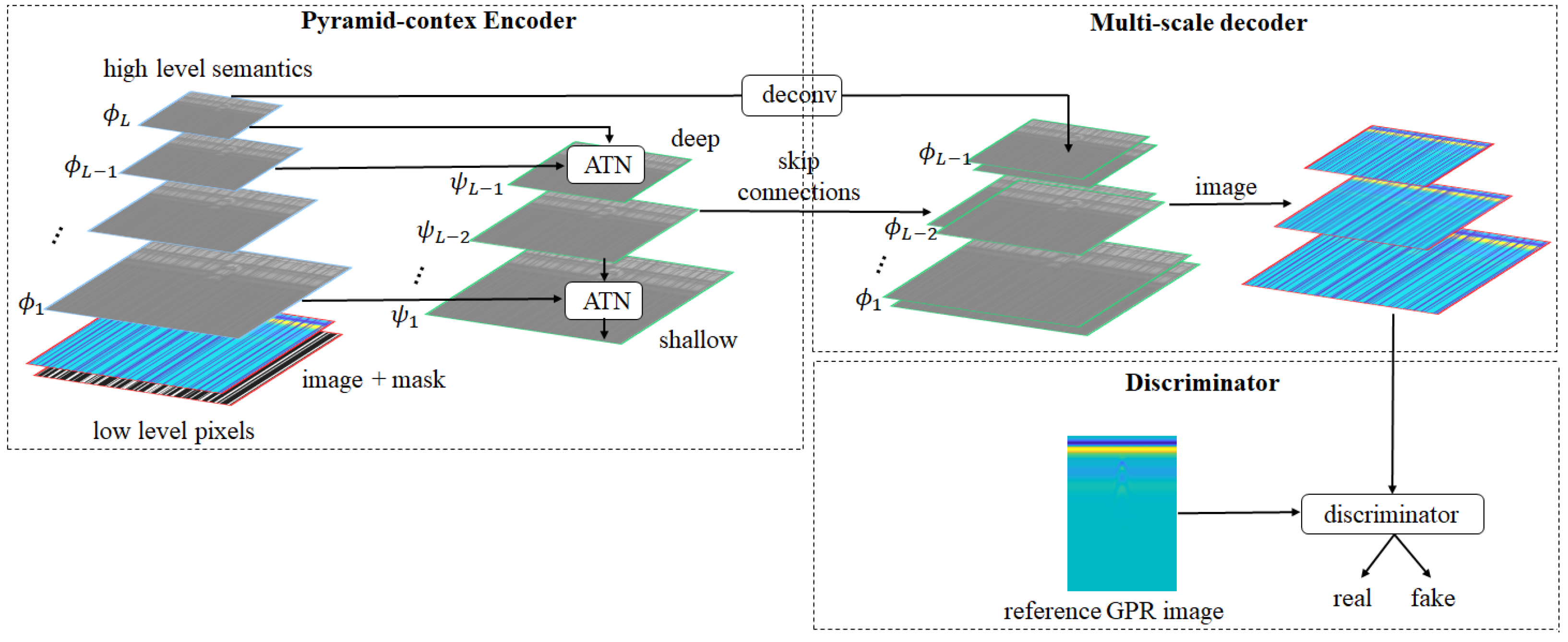
Deep generative models for image inpainting usually encode an image into a latent feature, fill missing regions at the feature-level, and decode the feature back into an image. PEN-Net consists of three main parts. The first part, Pyramid-context Encoder, is constructed with U-Net architecture  [44]. Specifically, missing regions on an image are encoded with masks, which are constructed from learned semantic features. While encoding latent features with the semantics of an image, missing regions are filled with a low-level feature map which is constructed by transferring rich details from a high-level feature map. This improvement is provided by embedding Attention Transfer Network (ATN) to each layer of the encoder since an ATN can memorize the similarity between patches that are located inside and outside of a missing region. Between these patches, an ATN learns textures with high-level features, and this information is used for padding missing regions [38]. The purpose of this is to use the learned similarity as a map to build a feature transfer for missing regions, assuming that similar pixel semantics would lead to similar textures  [45].

An illustration of PEN-Net architecture is given in Figure 2. Faithful to the notations and definitions given in  [45], $f(·,·)$ are defined as ATN operation, $\varphi$ as a feature map from deeper to shallow levels for L number of layers. Then, ATN applications can be formulated as follows.

$$\begin{array}{cc}\hfill {\psi }^{L-1}& =f({\varphi }^{L-1},{\varphi }^L),\hfill \\ \hfill {\psi }^{L-2}& =f({\varphi }^{L-2},{\psi }^{L-1}),\hfill \\ \hfill & ⋮\hfill \\ \hfill {\psi }^1=f({\varphi }^1,{\psi }^2)& =f({\varphi }^1,f({\varphi }^2,\cdots f({\varphi }^{L-1},{\varphi }^L))).\hfill \end{array}$$

(4)

For missing areas in the image, filling operations are performed (as in  [38,39,40]) by simply transferring related features from outside regions to inside of the missing regions. The application of this step is based on learning high-level feature maps.

$${\theta }^{*}=\underset{\theta }{\mathrm{argmin}}E\left(f_{\theta }(X;M)\right),$$

(5)

where

$$X^{*}=f_{{\theta }^{*}}\left(y\right).$$

(6)

In the second part of the model, a multi-scale decoder is considered. Here, high-level textures are fed to the decoder directly from the pyramid-context encoder, and low-level features are fed from ATNs as depicted in Figure 2. A combination of low-level features and high-level texture information provides building objects that are even missing in the masked region  [45].

$$\begin{array}{cc}\hfill {\phi }^{L-1}& =g({\psi }^{L-1}\oplus g\left({\varphi }^L\right)),\hfill \\ \hfill {\phi }^{L-2}& =g({\psi }^{L-2}\oplus g\left({\phi }^{L-1}\right)),\hfill \\ \hfill & ⋮\hfill \\ \hfill {\phi }^1& =g({\psi }^1\oplus g\left({\phi }^2\right))\hfill \end{array}$$

(7)

In the last part, a Patch-Generative Adversarial Networks (Patch-GAN) is integrated as the discriminator  [46]. Similar to conventional GANs, Patch-GAN is used to create similar images such that the discriminator can not distinguish a real image from a fake image that the generator has created, but it works on patch level.The discriminator is run over the image and created patches are merged to form the image. Since patch sizes are much smaller compared to the whole image, patch-GAN has fewer parameters, thus it is faster.

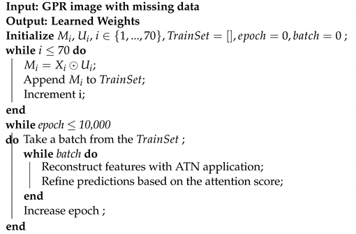
The algorithm regarding missing data recovery with PEN-Net on GPR data is given in Algorithm 1. At first, specially designed masks, $U_i\in {\mathbb{R}}^{m\times n}$ are applied to input GPR data, $M_i\in {\mathbb{R}}^{m\times n}$ corrupted GPR data matrices are obtained. These data are assigned to $TrainSet$. Afterwards the complete $TrainSet$ is forwarded to the model. At the end of the specified epoch, learned weights are obtained.

Algorithm 1: PEN-Net training algorithm on GPR Images.

3.2. Proposed DIP-Based Missing Data Recovery

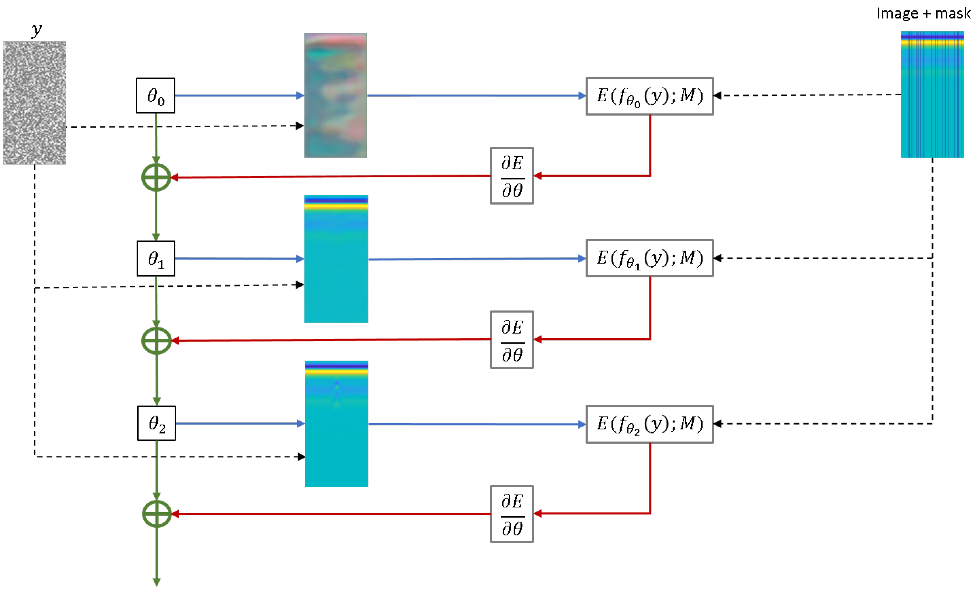
In DIP method, it is intended to examine the image before learning any of the parameters, which are obtained with a certain generator network structure. This is handled by optimizing the neural network in terms of parameter set, for an image $X=f_{\theta }\left(y\right)$, where image is $x\in {\mathbb{R}}^{1\times H\times W}$, code vector is represented as $y\in {\mathbb{R}}^{C^{\prime }\times H^{\prime }\times W^{\prime }}$, and network parameters are represented as $\theta$. Here, H and $H^{\prime }$ are used for height, W and $W^{\prime }$ for width and $C^{\prime }$ for code tensor.

In DIP, inverse tasks are examined such as denoising or inpainting, in order to show power of parametrization. Inverse applications can be explained as energy minimization problems, as follows (Figure 3)

$$X^{*}=\underset{X}{min}E(X,M)+R\left(X\right),$$

(8)

where $E(X;X_0)$ represents data term of the missing data recovery task, $x_0$ represents corrupted image and $R\left(X\right)$ term represents regularization term.

In these applications, regularization term is helpful for grasping the generic prior of images. However, most of the times regularization term is hard to identify. Simply, a regularizer can be a Total Variation (TV), which is the measure of the complexity of an image with respect to its spatial variation. In DIP application, this term is re-defined as the implicit image prior, which is created by the neural network as follows

Here, ${\theta }^{*}$ is the minimizer factor and gradient descent can be used as an optimizer to obtain ${\theta }^{*}$. For a given parameter set ${\theta }^{*}$, recovered image can be represented as $X^{*}=f_{{\theta }^{*}}\left(y\right)$. Taking into consideration (5) in terms of (8), the regularizer $R\left(x\right)=0$ for all images that can be generated by a deep convolutional network with a certain architecture. Considering that the network is not pre-trained with any data in this approach, image priors can be generated explicitly.

Images with missing data can be expressed as Hadamard’s product of a mask with an image. Assuming that the mask is composed with binary values such as $m\in {\{0,1\}}^{H\times W}$, then the data term of the masked image can be written as follows

$$E(X;M)={\parallel (X-M)\odot u\parallel }^2,$$

(9)

where $(x-x_0)$ represents corrupted image and ⊙ represents Hadamard’s product. In (9), missing pixel values are not involved and if the optimization would be performed over pixel values of the image, energy value would remain steady. Because of this reason a data prior is required and it is calculated by optimizing the data term with respect to (5). The recipe for the DIP method is presented in Algorithm 2.

Algorithm 2: DIP training algorithm on GPR Data

SkipNet is used, since skip connection provided adequate flexibility to capture image semantics. SkipNet, is consisted of convolutional networks and based on a given input, specific layers are inserted or discarded. In this model gating modules that are positioned each layer make binary decisions based on the activation from previous layer.

Binary decisions of gating modules are used to specify which layer will be run or discarded, as in Figure 4. Simply, output of the gated layer or layers can be calculated faithful to the notations in [47] as follows

$$x^{i+1}=G^i\left(x^i\right)F^i\left(X^i\right)+(1-G^i\left(x^i\right))x^i,$$

(10)

where $x^i$ is the input, $F^i\left(x^i\right)$ is the output of the $i^{\mathrm{th}}$ layer or layers and $G^i\left(x^i\right)\in \{0,1\}$ is the gating function of the $i^{\mathrm{th}}$ layer.

Remark: An ideal image is expected to be without noise or corruption. So for a neural network, image priors are used as references to perform a task such as denoising, missing data recovery or super-resolution. For this purpose, image priors can be generated by two approaches. In the first approach, a neural network can be trained with a dataset that is consisting of complete and corrupted images for missing data recovery application. Throughout the training, the model produces complete images at the output and it can be said that the model learns the prior from the dataset. Priors obtained with this method are called as learned priors. The drawback of this method is that a large dataset that includes both corrupted and complete images is necessary. In the second method, priors are generated from the corrupted image itself and the priors that are obtained with this method are named as explicit/handcrafted priors. In the scenarios where limited samples or a single sample exist, handcrafted priors have more advantages than learned priors, since handcrafted priors do not require a data set for training.

4. Experimental Results

In the experimental part, 2 different type of missing data cases (pixel-wise and column-wise) are compared for varying missing rates by using both conventional and deep learning-based methods in terms of visual and quantitative analysis. Both simulated and real datasets are used to test the limitation of the methods. In the simulated dataset, there are several GPR images, thus together with the conventional methods as GoDec, NMC, LmaFit, and NNM both PEN-Net and DIP models can be performed since PEN-Net needs training. However, the real datasets are limited and PEN-Net is not suitable since it requires training. For the real datasets, we only performed DIP model and the best performer of the conventional methods, NNM, for the sake of simplicity.

The quantative analysis is conducted through peak signal-to-noise ratio (PSNR) metric which can be given as

$$\mathrm{PSNR}\left(\mathrm{dB}\right)=10\log \left(\frac{1}{\left(\mathrm{MSE}\right)}\right)$$

(11)

Mean square error (MSE) can be formulated as

$$\mathrm{MSE}=\left(\frac{1}{m\times n}\sum _{i=1}^m\sum _{j=1}^n{\left(\mathbf{X}(i,j)-{\mathbf{X}}_{\mathrm{r}}(i,j)\right)}^2\right)$$

(12)

where i and j denotes the index terms. $\mathbf{X}$ and ${\mathbf{X}}_{\mathrm{r}}$ are the original raw GPR image, and the reconstructed GPR image after applying matrix completion, respectively.

4.1. Implementation

In our study, pipeline is implemented and executed on our workstation running a 64-bit Windows 10 Intel Core i7-8700K CPU with a 3.70-GHz clock, 64 GB RAM, and an NVIDIA GeForce RTX2080 Ti Super GPU. Python3 is used as programming language with PyTorch deep learning framework. For PEN-NET, hyper-parameters are selected as follows; for optimization, Adam optimizer is selected, the learning rate is set to 1 × 10${}^{-4}$, the batch size is kept as 16, and the number of iterations are set to 5 × 10${}^4$. All image sizes are kept original as 256 × 183. PEN-Net architecture is adapted from publicly available repository (https://github.com/researchmm/PEN-Net-for-Inpainting, 14 December 2021). For DIP, SkipNet with $dept=4$, which was the best performing choice in our trial, is selected. For padding and optimizer, zero padding and Adam optimizer are selected. Number of iteration is set as 10,000, learning rate is set to 0.01. Number of the parameters in the model is calculated as 1,060,739, as depicted in Figure 5.

4.2. Simulation Dataset Results

In this study, GPR images used for missing data recovery task are generated by the gprMax simulation software [48]. In the simulation setup, the buried object is a single aluminum target with the dielectric constant (F/m) as 3.1 and conductivity (S/m) as 2.3 × 10${}^7$, thus target signature can be clearly observed as a hyperbolic structure. Also surface and soil types are considered as flat and dry sand soil, where the dielectric constant (F/m) is 3.0 and conductivity (S/m) is 0.001 for the soil. Designed simulation setup and sample generated image are depicted in Figure 6. As seen in Figure 6, aluminum disk is used with dimensions 2.5 cm × 2 cm in radius and height. It is buried at 2 cm depth. The discretization of the model is selected as $\Delta x=\Delta y=\Delta z=1$ mm and the simulation domain is defined as $1000\times 120\times 400$ mm. Antennas are placed 5 cm above the ground, and moved 1 cm in each simulation to obtain A-scan along horizontal direction. In each scenario, antennas are moved 80 times to obtain the GPR image thus there are 80 A-scans and each A-scan contains 256 samples. Therefore, scanned distance is 80 cm, and it starts from 10 cm to 90 cm. The final obtained simulated GPR image has size $256\times 80$ and it is in gray scale. As an antenna type, commercial Geophysical Survey Systems, Inc. (Nashua, NH, USA), 1.5-GHz antenna (Model 5100) is used.

In order to present a comprehensive examination for missing data recovery, missing data scenarios are considered in 2 groups. In the first group, images with missing entries are generated by randomly selecting the pixels at different missing rates. In the second group, a similar approach is applied as missing column-wise pixels (randomly selected A-scans are removed). All matrix completion/data recovery methods use pixel-wise missing case although it is not feasible for practical measurements. Column-wise case is most encountered in field studies where at some measurement locations the complete response is missing. It is also possible to have some missing time samples in the A-scan response, this case can be thought as pixel-wise missing case.

4.2.1. Pixel-Wise Missing Data Case

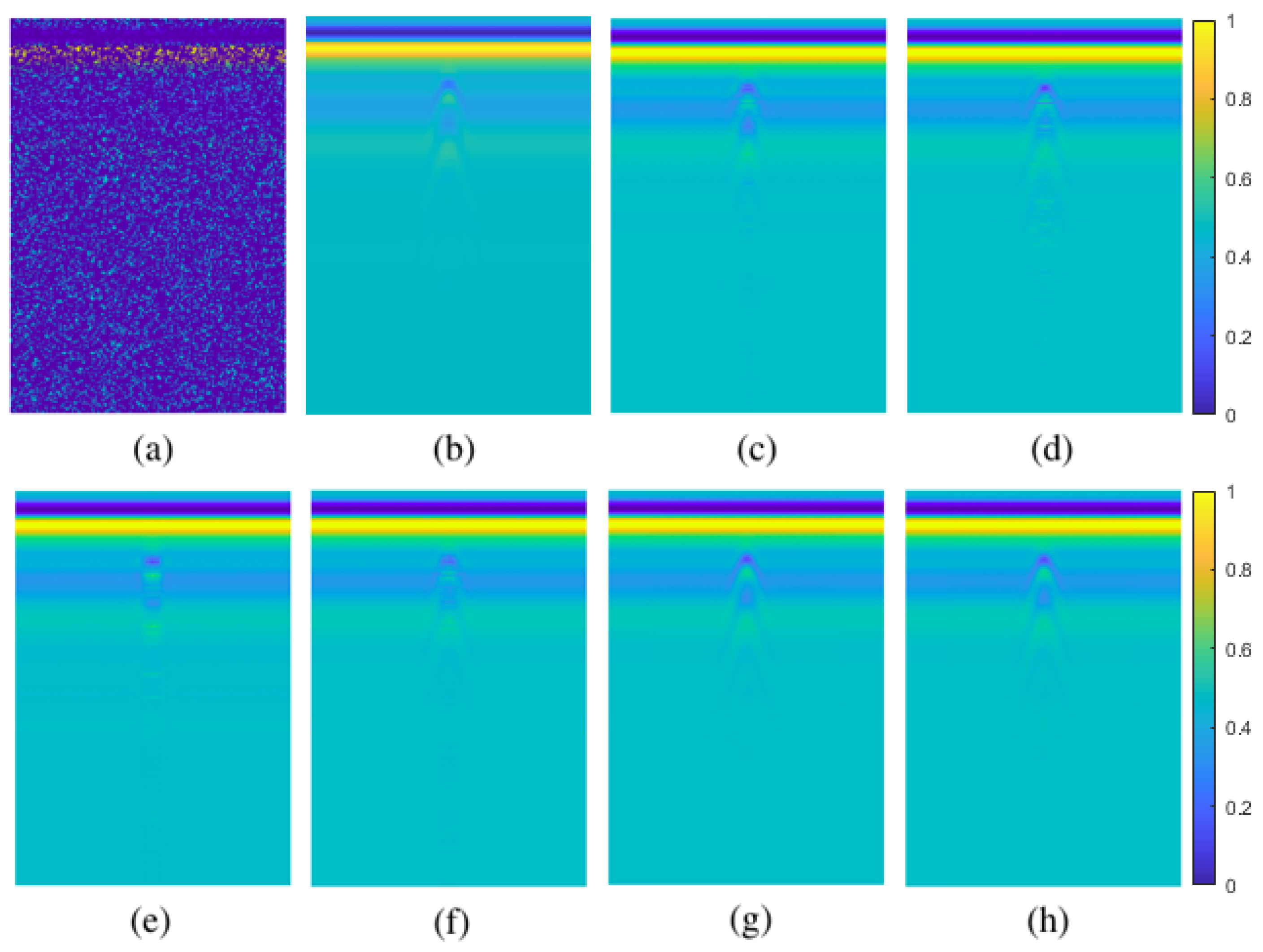
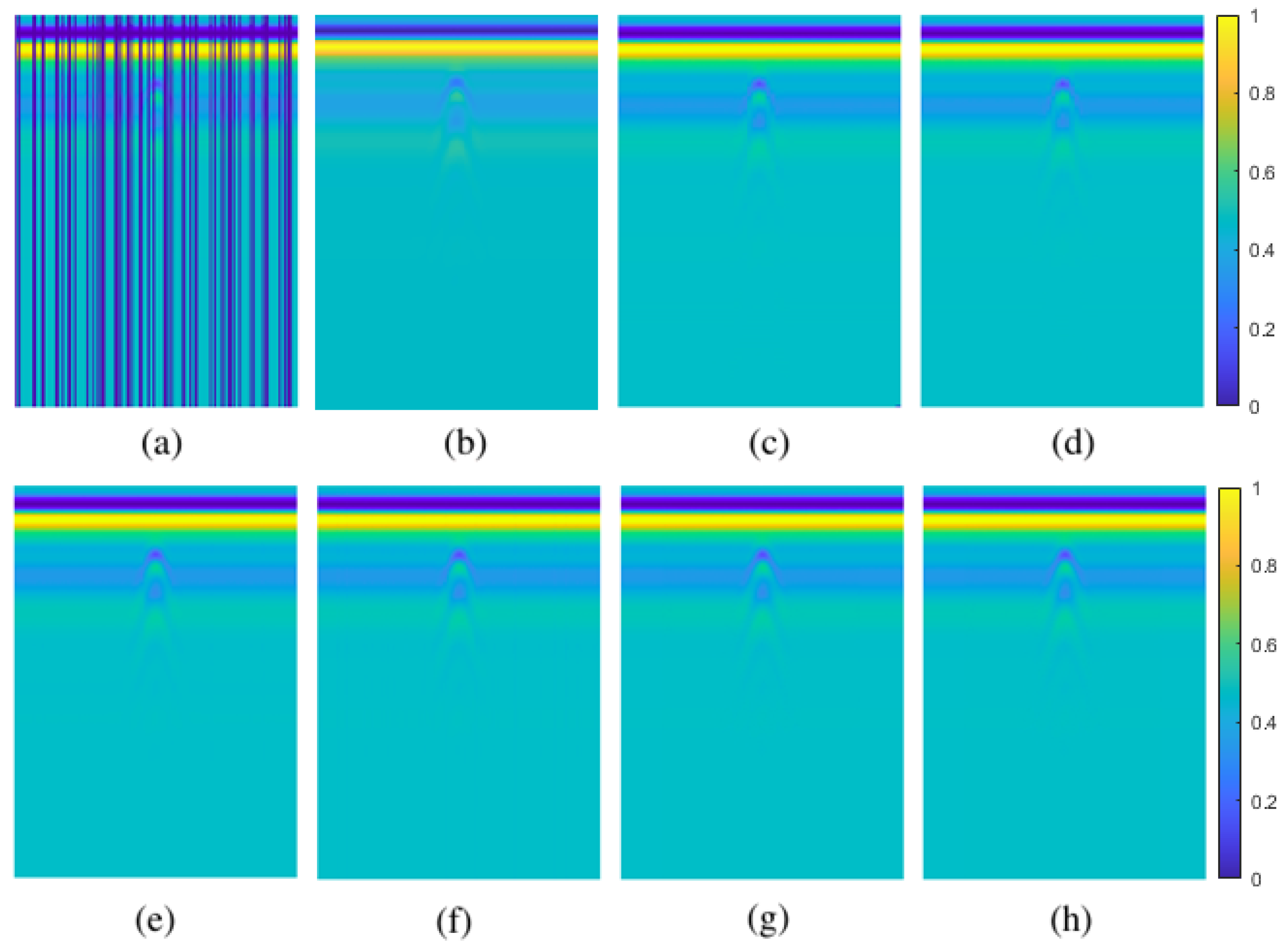
In pixel-wise missing data scenario, randomly selected pixels are corrupted with levels of $30\%,50\%$ and $80\%$, as depicted in Figure 7a, Figure 8a, and Figure 9a. Results are evaluated in both quantitative and visual aspects.

The simplest scenario is selected as $30\%$ missing rate for the pixel-wise case. The GPR image with missing pixels is shown in Figure 7a and the original GPR image is shown in Figure 7b. Even in this simplest scenario, the target signature is partially corrupted by the missing pixels compared to the original GPR image. Conventional methods and proposed methods are applied to the missing data to recover the original GPR image and the results are shown in Figure 7c–h. In the obtained visual results, it is hard to discern a difference between algorithms, however the visual results of DIP method seem more appealing compared to others. Since this scenario is the simplest one and the best performing algorithms from conventional methods are compared with the deep learning based methods, visual results are not helpful in terms of selecting the best method.

The scenario in Figure 8a is the moderate one and its original version is given in the Figure 8b. Again the visual results are similar to each other as given in Figure 8c–h. This phenomenon is also reasoned by the simulated data itself. Since the data is generated by simulation software, there is not much variation in the background and it is hard to catch visual differences by the result of the algorithms.

The missing scenario in Figure 9a is the challenging one even for the simulated data and its original version is given in the Figure 9b. As seen in the missing GPR image, the target can not be seen visually. When the results of conventional methods are visited, it is observed that NMC and LmaFit do not produce satisfactory results as seen from Figure 9d,e and there is a heavy distortion on the target signature however LmaFit is slightly better than the NMC in visual sense. The target signature in the NMC result has lost its hyperbolic structure thus it is the worst results among them all. The best results for the conventional methods are obtained by GoDec and NNM as given in Figure 9c,f where NNM is slightly better than GoDec since there is only small distortion in the target signature. PEN-Net and DIP perform well enough for this challenging data as given in Figure 9g,h and the latter one is better since it keeps the target signal strength.

For quantitative analysis, obtained results for pixel-wise missing data cases are given in

Table 2. PNSR comparison of data recovery methods for pixel-wise missing data.

	Missing Rate (%)	GoDec	NMC	LmaFit	NNM	PEN-Net	DIP
	30	63.21	67.67	90.82	92.21	104.31	117.82
	50	61.98	62.13	72.93	69.47	73.26	93.22
	80	47.25	42.02	43.60	48.34	45.79	57.77

for each missing rate. As expected, the performances of the algorithms are decreasing with respect to increasing missing rates and there is a dramatic decrease for 80% missing rate which is the most challenging scenario. When the quantitative results are analyzed, the first noticeable method is DIP which outperforms other methods for all the considered missing rates. Its closest follower is PEN-Net method, however, DIP is better than PEN-Net between 13–27% in terms of PSNR score. Both deep learning based methods show relatively higher performance compared to conventional methods. Only NNM and GoDec have slightly better performances than PEN-Net for the 80% missing rate. For the remaining ones, proposed methods present considerably higher performances and DIP takes the first place.

It can be concluded that from simple to challenging pixel-wise missing rates, the proposed methods perform far better than conventional methods and DIP algorithm heavily outperforms the other algorithms.

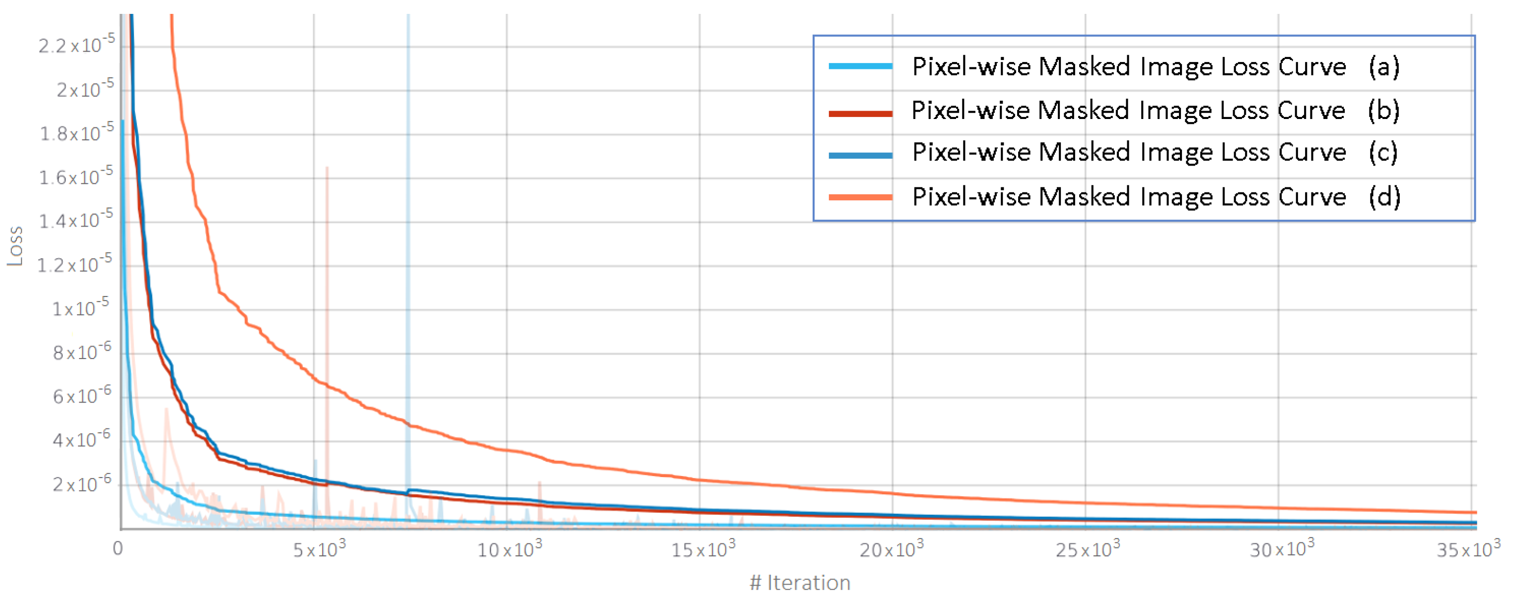
In Figure 10, Different curvatures for different levels of missing data are observed. With the higher corruption on the image, loss function converges to the highest error value and requires a higher number of iterations to converge to a steady value. The highest convergence is observed on the softest case, $10\%$ pixel-wise missing data. In the long run, error value converges to a lower value. Hence, for the proposed method, direct relationship between the decreasing trend in PSNR values can be represented with the loss curves.

4.2.2. Column-Wise Missing Data Case

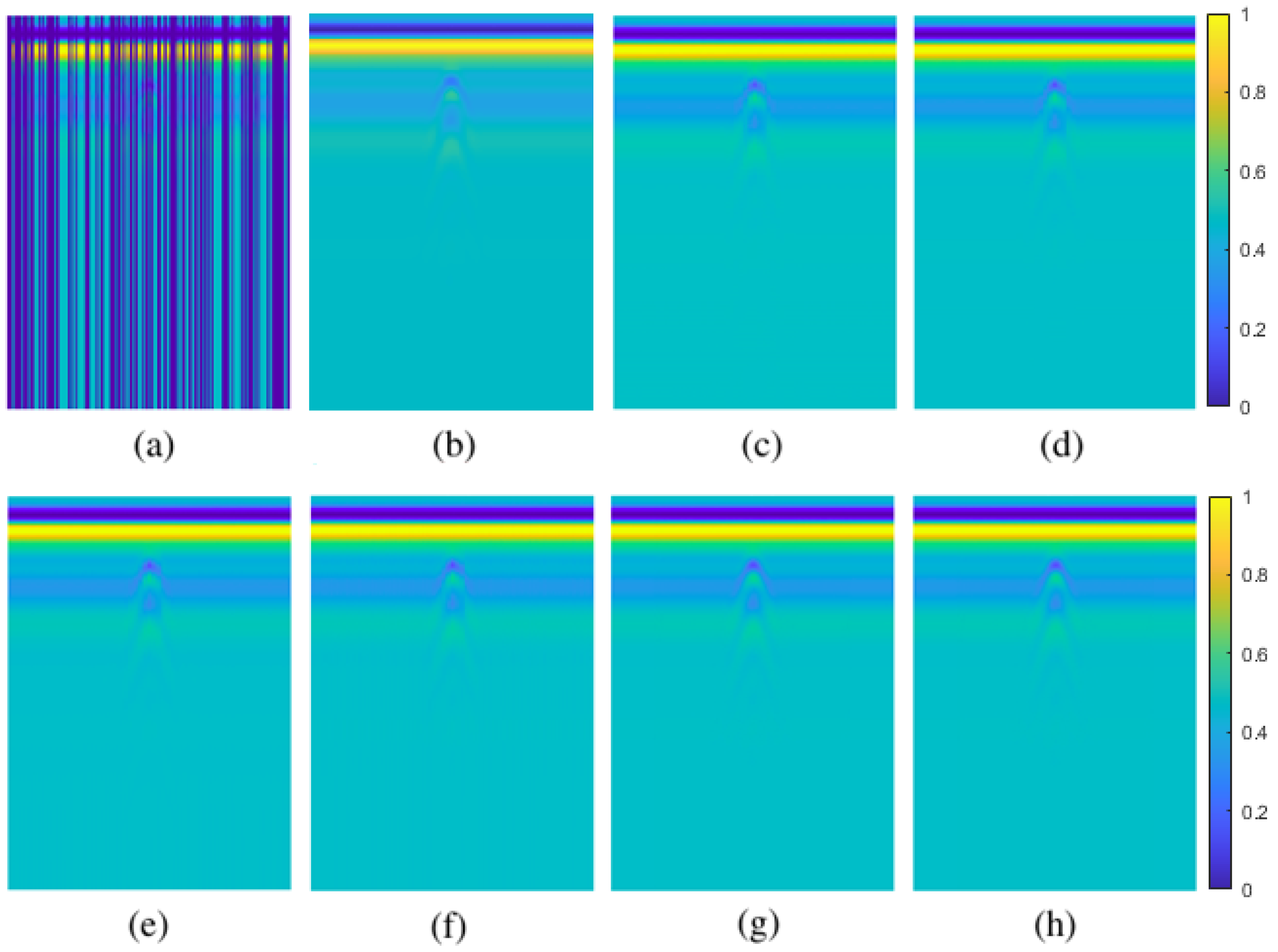
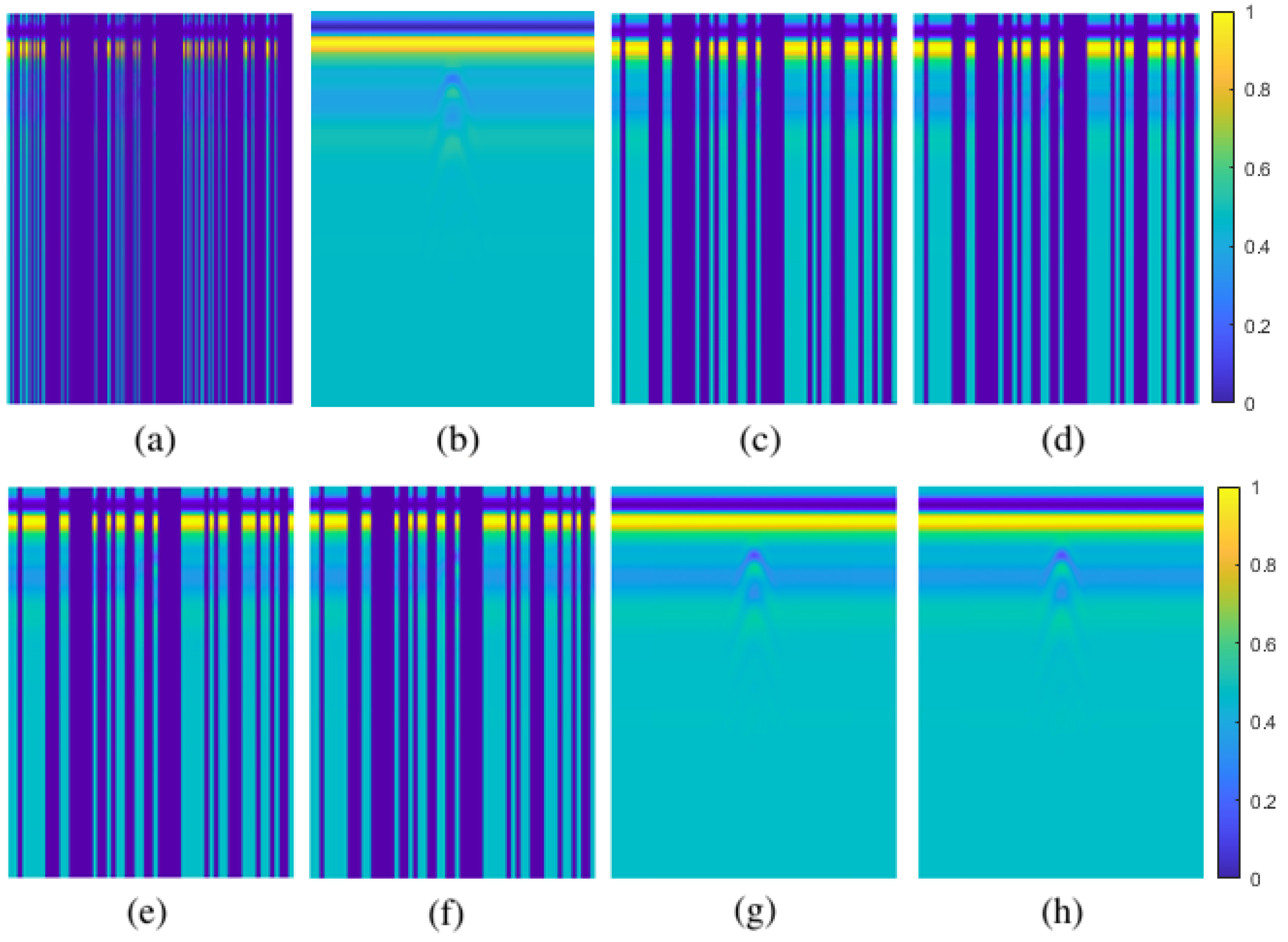
In the column-wise missing data scenario, randomly selected columns are corrupted from the image with levels of $30\%$, $50\%$ and $80\%$, as given in Figure 11a, Figure 12a, and Figure 13a. Recovered images are examined in visual and quantitative aspects.

As in the pixel-wise missing case, the simplest scenario is started from $30\%$ missing rate for column-wise missing data and this is presented in Figure 11a. The original raw GPR image is given in Figure 11b. As seen in the column-wise missing image, the target signature can be partially observed. The visual results are quite similar since this is the simplest scenario as seen from Figure 11c–h. All the methods have successfully recovered the missing GPR image entries. Thus it is hard to choose the best performing algorithm from visual results.

The missing scenario in Figure 12a is the moderate one, however the target seems highly corrupted by the missing A-scans compared to the given original raw GPR image in Figure 12b. When the visual results of the algorithms are analyzed, it is observed that conventional methods have performed similarly as given in Figure 12c–f, however all of them cause some undesired distortion on the target signature. The proposed methods preserve the hyperbolic structure of the target signature as presented in Figure 12g,h and the DIP method has a slightly better performance in visual sense.

The missing scenario in Figure 13a is the challenging one and the target is not seen from the missing GPR image compared to the given original raw GPR image in Figure 13b. Since, the missing number of columns is so high, some of them concatenate to each other and it becomes block-wise missing data instead of a column-wise. The results of conventional methods are presented in Figure 13c–f. As seen in the results, some of the missing columns are still available and this is reasoned by the block-wise missing data regions. According to matrix completion theory, the conventional methods need at least one observation for each row and column after pre-transformation. However the block-wise missing data regions violate this theory thus the region can not be recovered by these algorithms. The proposed methods do not need pre-transformation step and they successfully recover the missing GPR image even in the block-wise missing regions as seen from Figure 13g,h. Both PEN-Net and DIP algorithms present similar visual performance even in this extreme case while conventional methods fail to recover the missing GPR image entries.

In Figure 14, different curvatures are observed for different levels of missing data. With the higher corruption on the image, loss function converges to the highest error value. Also, it requires dramatically longer iterations to converge to a steady value. The highest convergence is observed on the softest case, $30\%$ column-wise missing data. In the long run, error value converges to a lower values. However, since column-wise missing data is a more challenging recovery case, loss curves of the $50\%$ and $80\%$ overlap and converges to their minimum levels after 15,000 iterations. Also, decreasing trend in PSNR values are interrelated with the loss curves.

The quantitative results for the column-wise missing case are presented in

Table 3. PNSR comparison of data recovery methods for column-wise missing data.

	Missing Rate (%)	GoDec	NMC	LmaFit	NNM	PEN-Net	DIP
	30	46.83	59.61	50.38	54.43	53.50	63.43
	50	49.51	50.43	49.53	49.30	54.68	57.63
	80	–	–	–	–	30.55	31.19

. As seen from the table, the best results are obtained by the DIP method. PEN-Net outperforms the conventional methods except the first case. For the conventional methods, the best results are obtained by NMC and NNM follows it. The GoDec has the worst performance and LmaFit is slightly better than GoDec algorithm. However, all the conventional methods fail for the 80% missing rate. Overall, the best result is obtained by the DIP algorithm and it is 2–6% better than its closest follower.

4.3. Real Data Results

In this study, two challenging real data sets are used to further validate the effectiveness of the algorithms. As in the simulated case both visual and quantitative results are presented. Besides, For the challenging cases, the target parts are cropped and focused to further analyze the NNM and DIP performances.

4.3.1. Real Data-I

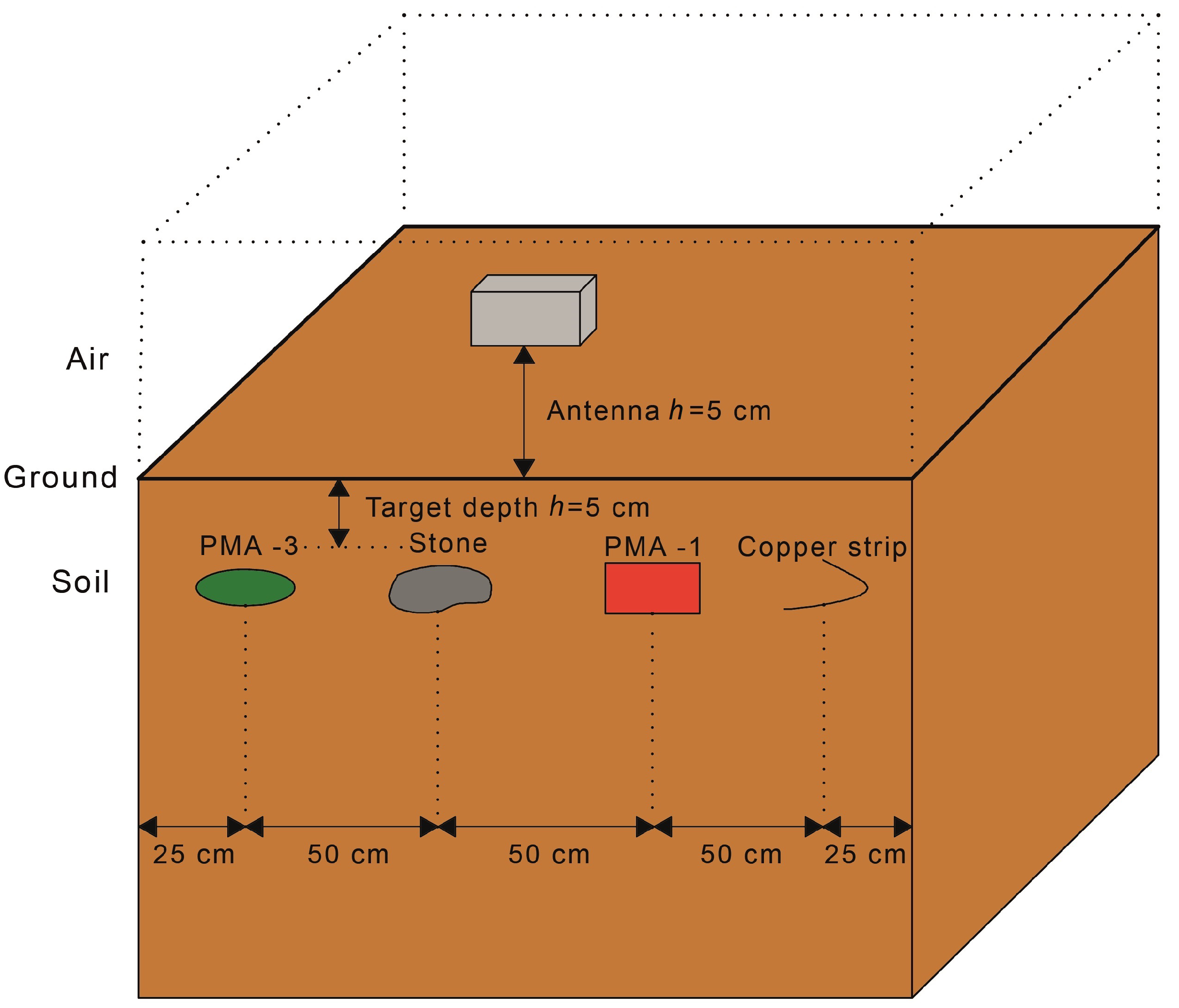
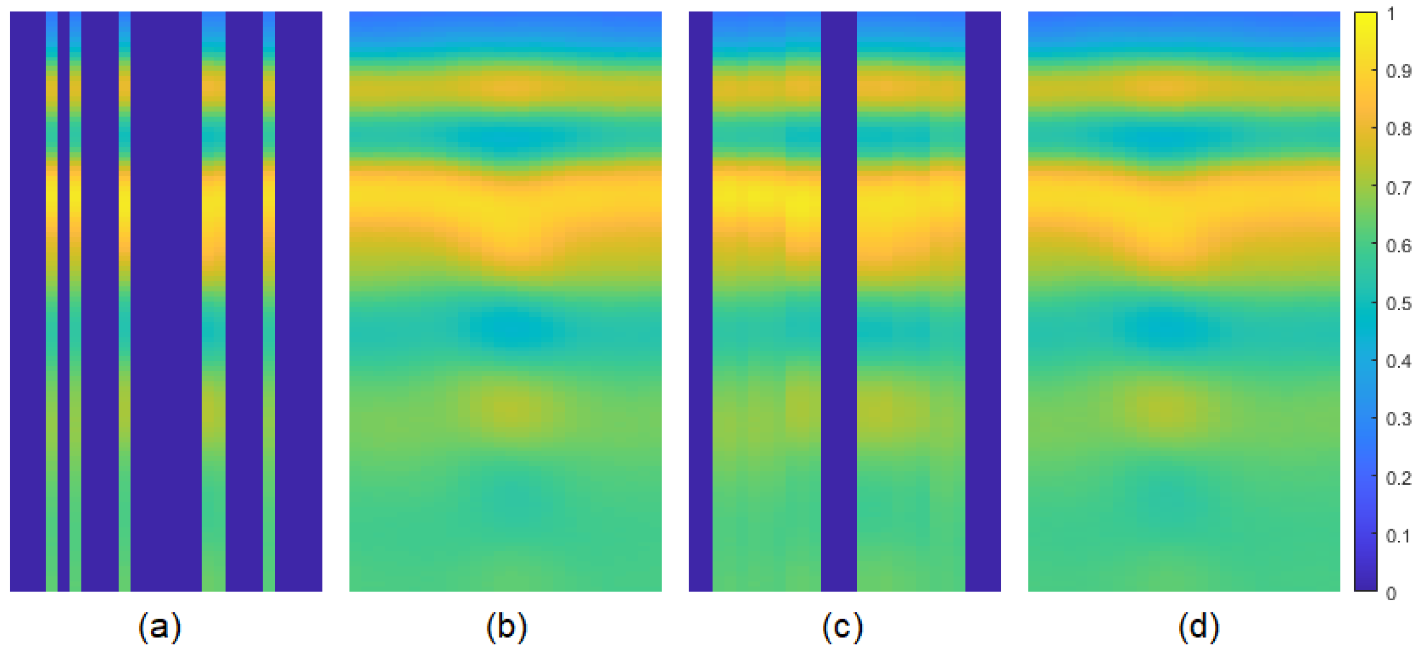
The first real GPR data from Vrije Universiteit Brussel is used for testing the algorithms for missing data cases. Its experimental design is shown in Figure 15 and the measured real data is given in Figure 16b. In this scenario, PMA-3, PMA-1, stone and copper strip targets are located at 5 cm depth where the PMA-3 and the PMA-1 refer to the plastic case antipersonnel landmines. The soil type is dry clay soil and it is mixed with small rocks, and there are irregularities on the surface with a maximum of 10 cm. An antenna is placed 5 cm above the highest point of the surface. An area of 50 cm × 196 cm was scanned with a scanning step of 1 cm in each direction. The final obtained real data has size $512\times 197$ and it is in gray scale. For the real data, there are irregularities in the background of the obtained raw GPR image and it makes the missing data recovery problem more challenging compared to the simulated data. Since, the background of the simulated data does not present many variations, the performances of the algorithms are higher with respect to the real data. Since we assume that a single B-scan is available as in most of the field studies, PEN-NET architecture trained for simulated data highly remains behind all the methods. Thus its results are not included in this section. The DIP algorithm does not need the training step hence it can be used for single image data recovery. Among the conventional methods, NNM algorithm is selected for comparison due to its high performance and parameter free feature.

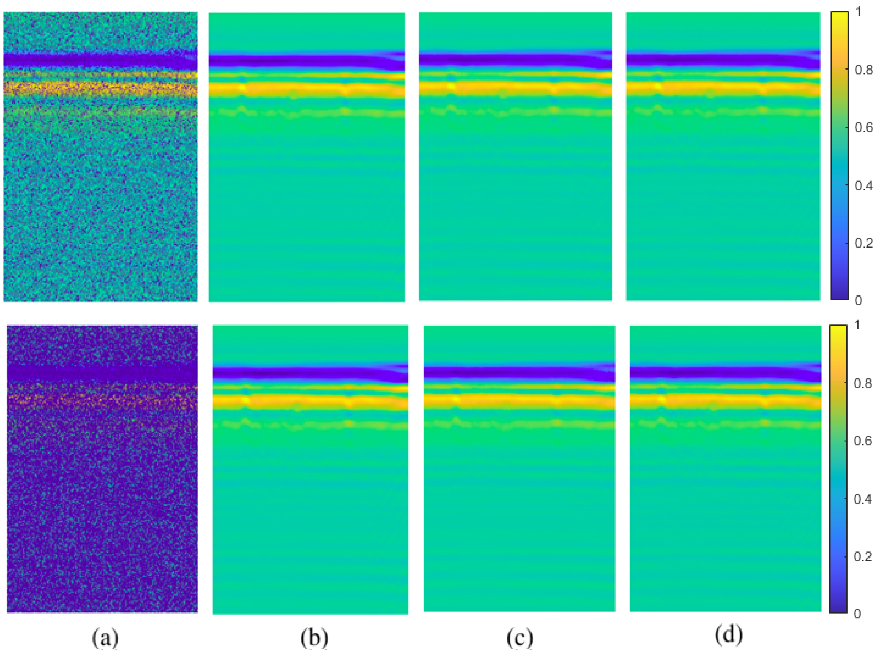
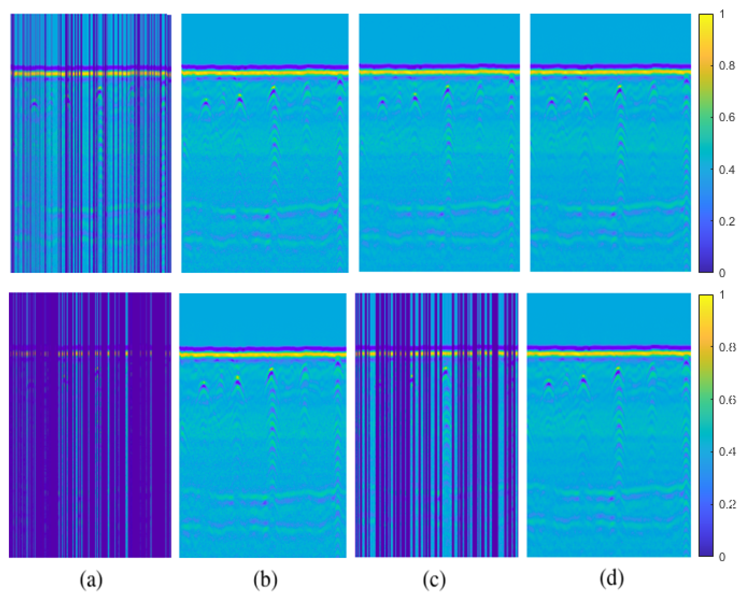
The first pixel-wise missing case is relatively simple and it is selected as $30\%$ as given in the first row of Figure 16a. The real GPR data is shown in Figure 16b. Since, this scenario contains 4 different targets, some of them are barely seen visually even in the original raw GPR data. The recovery results of NNM and DIP algorithms are shown in Figure 16c,d. This scenario is the simple one and best performing algorithms are selected for the real GPR data case thus both algorithms produce satisfactory results in the visual sense. It is hard to distinguish any differences between these results.

In the second pixel-wise missing case, a challenging case is selected to test the limits of the algorithms and it is presented in the second row of Figure 16a and its original GPR image is given in Figure 16b. The obtained results are shown in the Figure 16c,d where both of them produce satisfactory results. However, when the results are analyzed in detail, it can be observed that the target signatures are better preserved by DIP method.

For the quantitative analysis part, NNM and DIP have a similar performance for the simplest missing case ($30\%$) which are 59.51 dB, and 60.89 dB in terms of PSNR. The results shows that DIP method has slightly better performance than the conventional method NNM. For the challenging missing case, NNM is obtained 45.80 dB and DIP is obtained 51.1 dB which shows that DIP algorithm is approximately $12\%$ better than NNM algorithm for the extreme case. Thus, it can be deduced that when the missing rate is increased for the pixel-wise case, the performance gap between NNM and DIP increases proving the superiority of DIP for high missing rates.

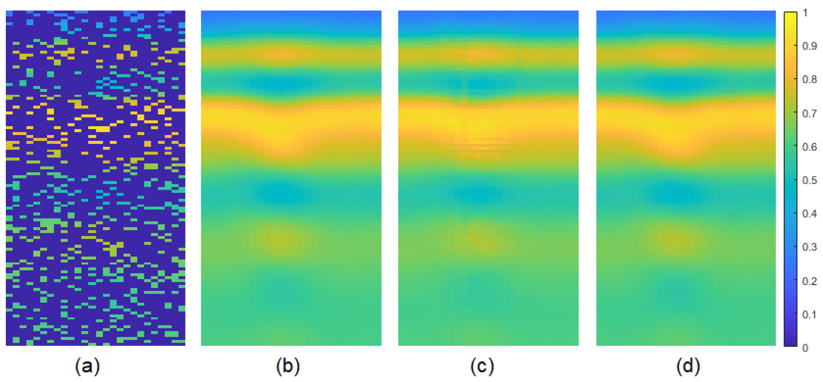
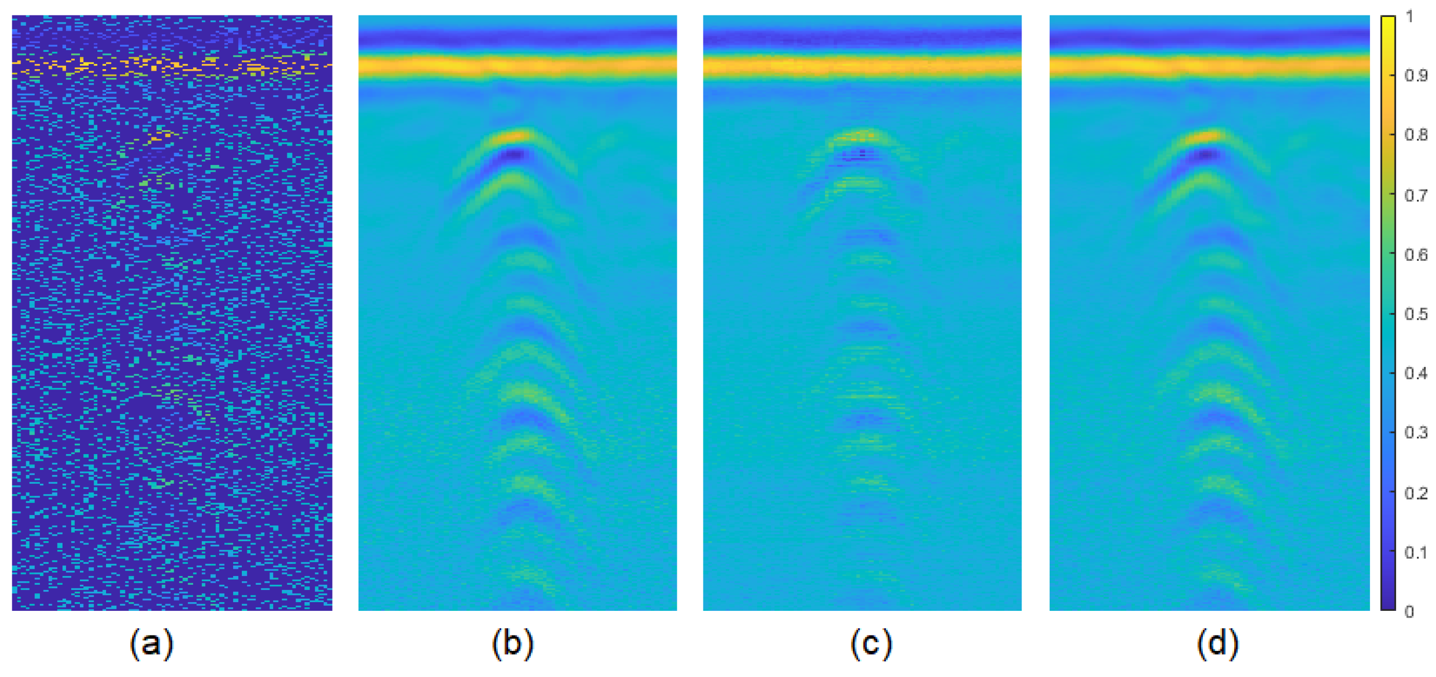
Generally, the background of the GPR image is simple and does not present many variations. For this purpose, an area around the target is cropped and visual results are shown in Figure 17a–d. It can be observed that NNM has some artifacts from missing informations however DIP results are smooth. The quantitative results are given in

Table 4. PNSR comparison of data recovery methods for pixel-wise missing case for real data-I.

Missing Rate (%)	NNM	DIP	NNM${}_{\mathit{z}\mathit{o}\mathit{o}\mathit{m}\mathit{e}\mathit{d}}$	DIP${}_{\mathit{z}\mathit{o}\mathit{o}\mathit{m}\mathit{e}\mathit{d}}$
30	59.51	60.89	–	–
80	45.80	51.12	34.24	47.36

. As seen from the table, the proposed DIP method show much better performance than NNM for the hyperbolic target shape recovery with respect to overall GPR results comparison.

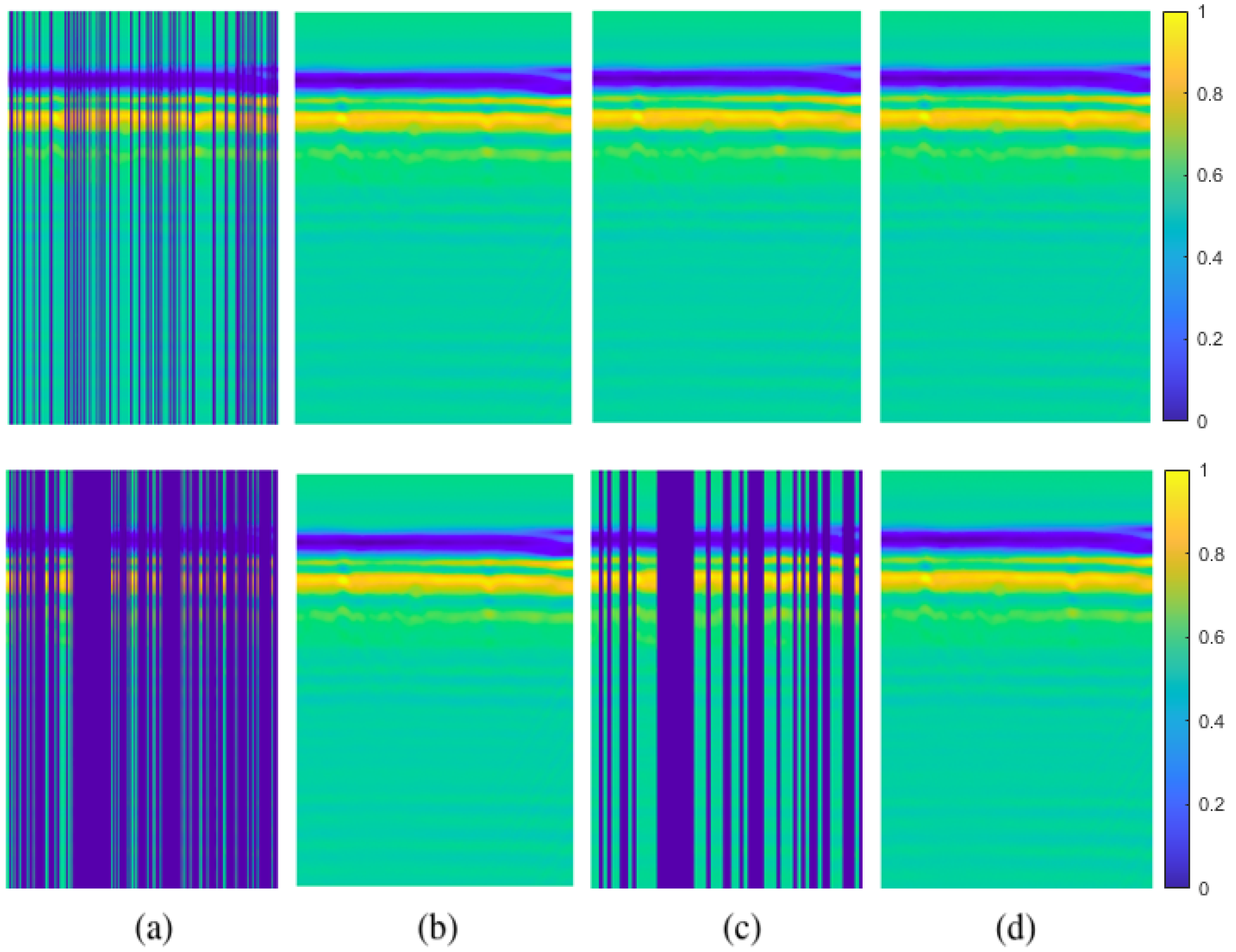
The first column-wise missing case is again the simple scenario and it is presented in the first row of Figure 18a where its original GPR image is given in Figure 18b. Since this is the simplest one, both NNM and DIP algorithms present satisfactory results as given in Figure 18c,d. In this missing case, the missing number of columns are comparatively less than the number of obtained A-scans, thus there is no block-wise phenomenon happening in this missing column-wise case. Thus, NNM can successfully recover the GPR image. However, when the recovered results are zoomed, it can be observed that DIP is slightly better in this simple case.

The second column-wise case is the challenging one as given in the second row of Figure 18a where its original GPR image is presented in Figure 18b. During the missing data case construction, the columns are randomly removed and as seen in Figure 18a, and some columns are concatenated. As a result, some of the areas are missing in blocks pointing out a situation which can occur in real life experiments. This phenomenon can corrupt the target partially or completely thus this extreme case is a good example to test the performances of the algorithms. The recovery results for this challenging scenario is presented in Figure 18c,d. As seen in the results, NNM can not handle the extreme scenario as expected. The block-wise regions affect the performance of NNM. However, DIP algorithm can successfully recover the missing data entries. Even the target signatures still keep their structures.

The quantitative results of the column-wise missing cases are parallel with the visual results as show in Table 4. For the simplest scenario, PSNR values given by NNM and DIP algorithms are 52.79 dB, and 58.99 dB, respectively. As seen from the results, DIP algorithm is approximately $12\%$ better than the NNM algorithm. The performance gap becomes more distinct for high missing data rate. PSNR values of NNM and DIP algorithms are 8.06 dB, and 33.64 dB, respectively. Actually, NNM algorithm fails to recover the missing GPR image for extreme case. As in the visual results, DIP algorithm outperforms the best performing conventional method for the column-wise missing cases.

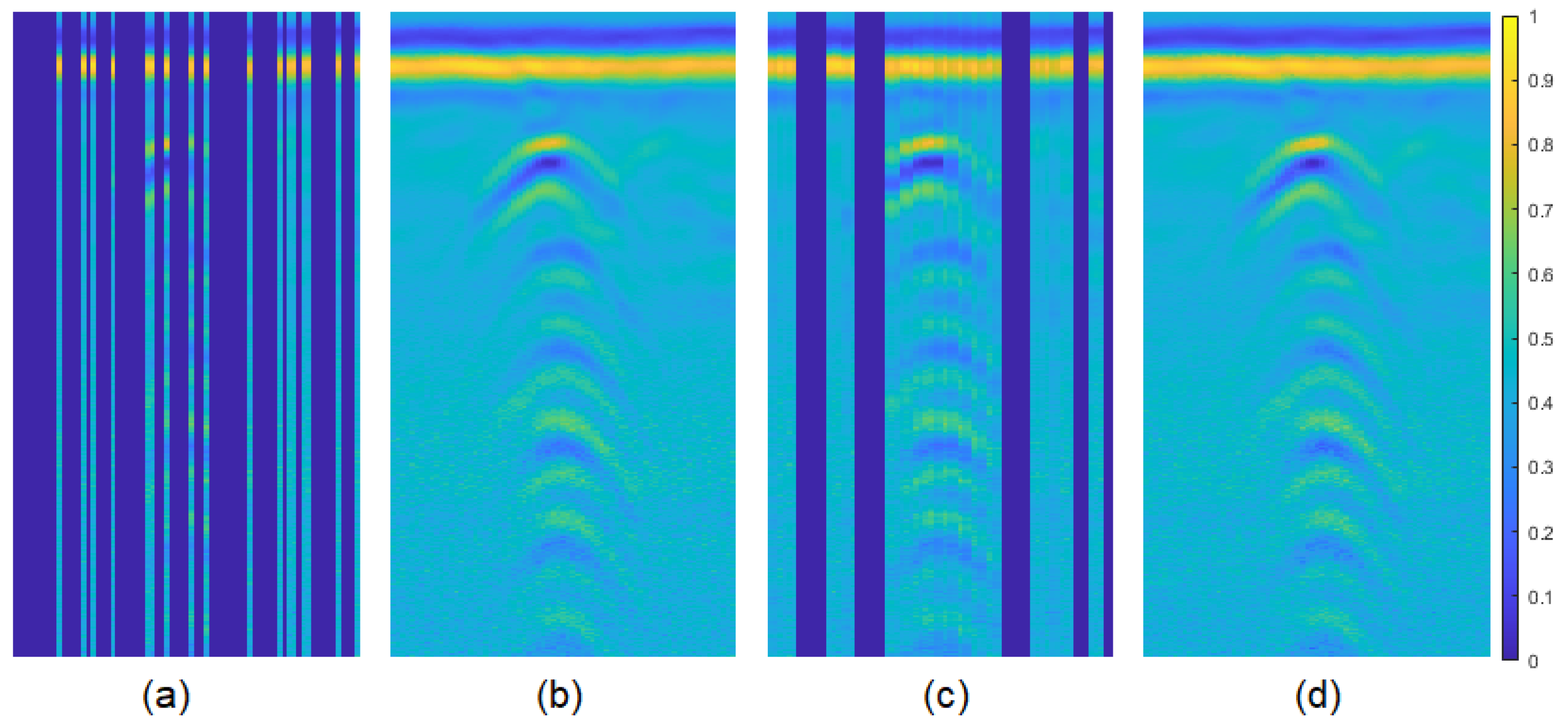
The zoomed results for the target (third one) is shown in Figure 19a–d. For this case, NNM fails to recover the GPR image as can be seen from the Figure 19c. However, DIP method can recover the hyperbolic target well enough. This can be also observed from the quantitative results in

Table 5. PNSR comparison of data recovery methods for column-wise missing case for real data-I.

Missing Rate (%)	NNM	DIP	NNM${}_{\mathit{z}\mathit{o}\mathit{o}\mathit{m}\mathit{e}\mathit{d}}$	DIP${}_{\mathit{z}\mathit{o}\mathit{o}\mathit{m}\mathit{e}\mathit{d}}$
30	52.79	58.99	–	–
80	8.06	33.64	12.05	32.28

. The gap between performance for this case is very distinctive since the NNM method did not recover the missing GPR image.

4.3.2. Real Data-II

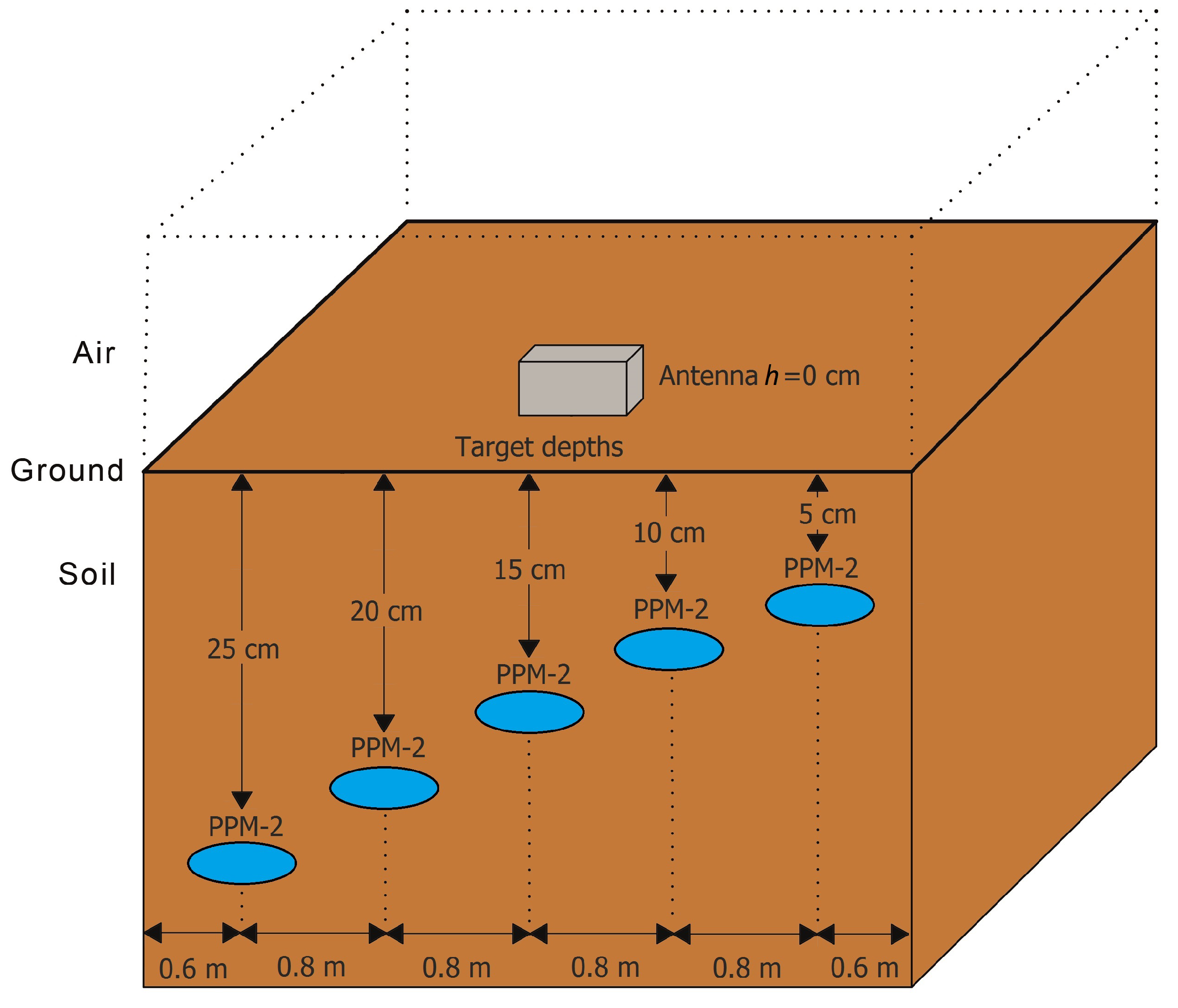
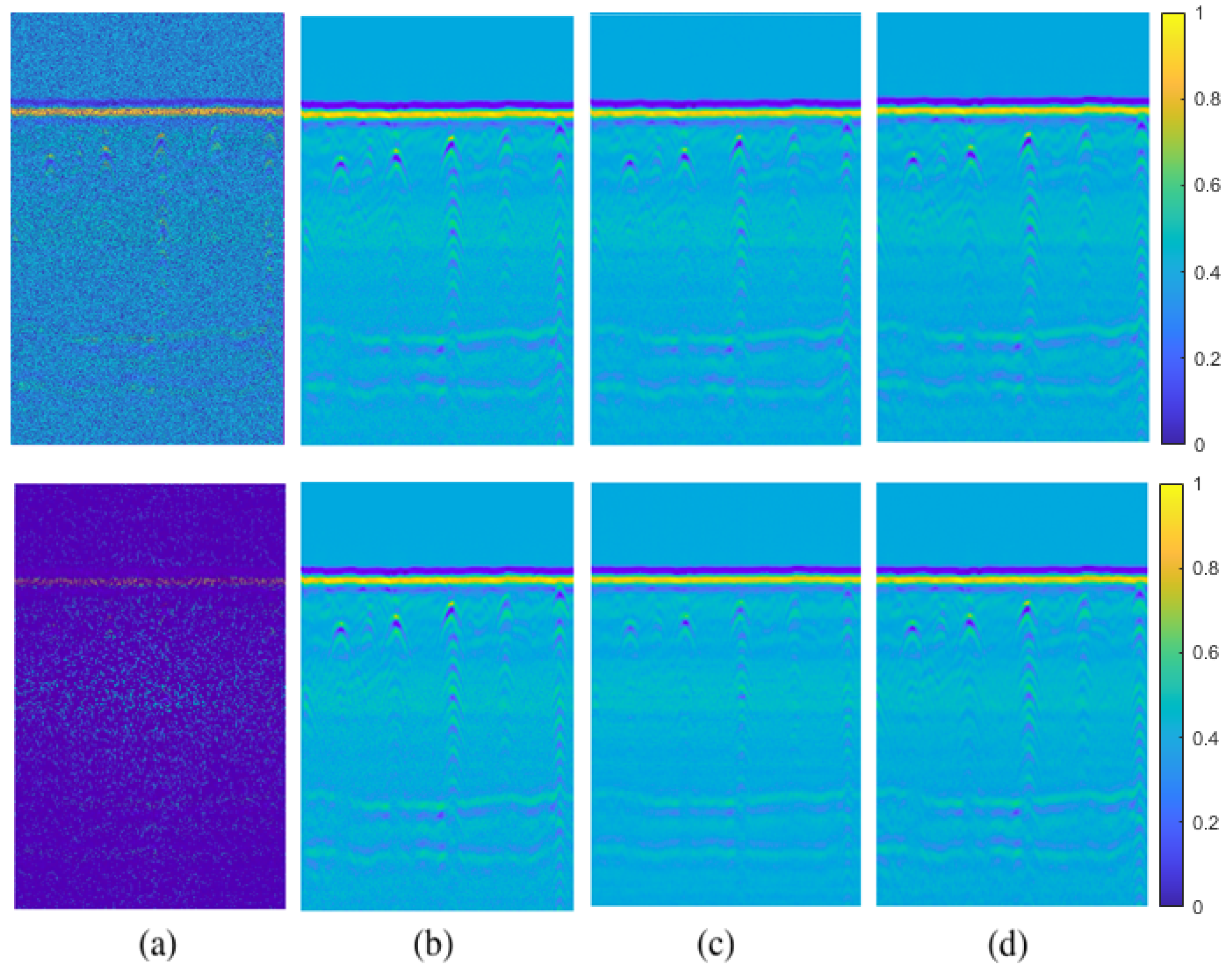
The experimental design of the second real scenario is given in Figure 20 and the raw data result is presented in Figure 21b. Field test measurements are obtained from demining operations conducted in Germany under the project of the International Test and Evaluation Program for Humanitarian Demining (ITEP) in 2009. In this particular operation, a commercial GPR antenna (SIR-3000 with 1.5-GHz antennas, GSSI) was used and it was located just over the ground. The antenna was moved over the centre of the landmines with a broadside in perpendicular orientation. Five rendered-safe landmines (PPM-2) which had the diameter of roughly 13 cm were buried in the same directions with different positions such as 0.6, 1.4, 2.2, 3.0, and 3.8 m. The burial depths of the objects was 25, 20, 15, 10 and 5 cm, respectively. The soil type was magnetic sand in order to replicate soil with high magnetic susceptibility. The texture is rough sand with a small amount of fine gravel. The final obtained real data has size $2049\times 401$ and it is in gray scale.

The first pixel-wise missing case is simple as in the real data-I. As seen from the first row of the Figure 21a, the target can be observed visually. Since this is the simplest scenario, both NNM and DIP algorithms performed well enough. As given in the Figure 21c,d, the results are visually similar to the original real data-II as presented in Figure 21b. It is hard to discern performance difference from the visual results for this missing case.

The second pixel wise missing case is challenging compared to the first case. As seen from the second row of Figure 21a, the targets are mot visible. When the visual results in Figure 21c are zoomed, it can be observed that the target signatures are attenuated compared to the results in Figure 21d. However, the visual results are still satisfying compared to the original real data-II in Figure 21b. In this extreme case, It can be deduced that DIP algorithm has a better performance compared to the NNM algorithm.

The quantitative results agree with visual results. For the simplest pixel-wise missing case, PSNR scores for NNM and DIP are 35.99 dB and 39.57 dB, respectively. DIP algorithm is almost $10\%$ better than the best performing conventional matrix completion algorithm NNM. For the extreme pixel-wise missing case, PSNR value for NNM algorithm is 30.41 dB while 33.04 dB for DIP. The DIP algorithm is again $11\%$ better than NNM algorithm which proves that making pixel-wise missing cases more difficult do not worsen performance, on the contrary, it improves.

For further analysis, the third target which has hyperbolic shape is zoomed and it is shown in Figure 22a–d. NNM result in Figure 22c seems blurry and the target signal strength was attenuated however DIP method keeps the target signature. This can be also seen from the quantitative results in

Table 6. PNSR comparison of data recovery methods for pixel-wise missing case for real data-II.

Missing Rate (%)	NNM	DIP	NNM${}_{\mathit{z}\mathit{o}\mathit{o}\mathit{m}\mathit{e}\mathit{d}}$	DIP${}_{\mathit{z}\mathit{o}\mathit{o}\mathit{m}\mathit{e}\mathit{d}}$
30	35.99	39.57	–	–
80	30.41	33.04	27.61	37.24

. The gap between the PSNR scores is more obvious for the zoomed version.

For the column-wise missing case, the simplest scenario is same with the real data-I. As given in the first row of the Figure 23a, the targets can be observed visually by comparing the original real data-II in Figure 23b. When the visual results are checked, it can be observed that both methods can perform well enough for the simplest column-wise missing scenario as expected. However, the target signatures are preserved by DIP algorithm compared to the NNM as presented in the Figure 23c,d.

The extreme column-wise missing case is shown in the second row of the Figure 23a and the targets are barely visible. Especially, the first and last two targets are completely corrupted by the missing columns compared to the original real data-II in Figure 23b. The visual results are presented in Figure 23c,d. NNM algorithm can not recover the missing columns as expected due to the high number of missing columns, the columns are concatenated into blocks and NMC fails at this part. However, DIP algorithm can successfully recover the missing GPR image even in the extreme case. The presented visual result in Figure 23d shows the efficiency of the recovery.

The column-wise missing case is more important than the pixel-wise missing case since the first one is more frequently encountered during field measurements. When the simplest column-wise missing case is checked, NNM algorithm gives 33.33 dB and DIP algorithm 36.37 dB as PSNR score. Again, DIP is better than NNM almost $10\%$ in quantitative sense. For the extreme column-wise missing case, NNM has 10.06 dB and DIP algorithm has 39.60 dB PSNR score. For this case, NNM fails to recover GPR image however DIP recovers even better than the simplest case which shows the superiority of the DIP over conventional matrix completion methods.

The zoomed version for the column-wise missing case is presented in Figure 24a–d. As seen from Figure 24d, DIP preserves hyperbolic shape of the target unlike NNM. This can be also observed from the quantitative results in

Table 7. PNSR comparison of data recovery methods for column-wise missing case for real data-II.

Missing Rate (%)	NNM	DIP	NNM${}_{\mathit{z}\mathit{o}\mathit{o}\mathit{m}\mathit{e}\mathit{d}}$	DIP${}_{\mathit{z}\mathit{o}\mathit{o}\mathit{m}\mathit{e}\mathit{d}}$
30	33.33	36.37	–	–
80	10.06	39.60	13.83	25.77

. DIP score is almost two times better than the NNM score.

The two methods are tested on the real data-II for $30\%$ column-wise missing case on Intel core i7 6700HQ @ 2.6GHz, 8GB DDR4-2133, Nvidia GTX950M, on a Windows 10 64-bit environment. NNM and DIP running times are 2.48 and 280 s, respectively. We should remark that for $80\%$ column-wise missing case, NNM fails while DIP recovers successfully the missing samples.

5. Conclusions

Two new methods which are based on deep networks have been proposed for data recovery in GPR: PEN-Net and DIP methods. PEN-Net due to its architecture learns from data through the training stage and needs only an adequate amount of data, while DIP combines an optimization procedure with a deep network structure with fixed coefficients used as a handcrafted prior. Similar to matrix completion based conventional methods, DIP does not require any training thus a single corrupted image is enough. As expected, deep learning method PEN-Net provides the fastest results (in the testing stage), DIP is more time consuming even with respect to the conventional methods. However, the performance of the conventional methods decrease drastically for high missing data rates where the proposed methods provide satisfactory results. In the simulated data experiments, the proposed methods outperform conventional methods for the challenging pixel-wise case around 17–27% and moderate level column-wise missing case around 15%. In addition, for the high rate of column-wise missing data cases where the conventional methods completely fail, they can still yield satisfactory results.

It can be concluded that the proposed methods can be good alternatives to matrix completion for high missing data rates, especially in column-wise data missing case which is more realistic in GPR. When an adequate number of measurements are available PEN-Net model can be used, while if data acquisition is limited to a few samples, a case more appropriate for real data measurements, and enough computational power exists, DIP method can be preferred. Moreover the current deep learning research is focused on explainable artificial intelligence (XAI) where the black box structures of the former studies are replaced by model driven or interpretable networks which combine optimization and generative networks [49,50]. DIP can be considered as a bridge between these two trends.

References

1. Daniels, D.J. Ground Penetrating Radar; IET: London, UK, 2004. [Google Scholar]
2. Devaney, A.J. Time reversal imaging of obscured targets from multistatic data. IEEE Trans. Antennas Propag. 2005, 53, 1600–1610. [Google Scholar] [CrossRef]
3. Ciuonzo, D.; Romano, G.; Solimene, R. Performance analysis of time-reversal MUSIC. IEEE Trans. Signal Process. 2015, 63, 2650–2662. [Google Scholar] [CrossRef]
4. Li, X.F.; Li, X.F. Seismic data reconstruction with fractal interpolation. Chin. J. Geophys. 2008, 51, 855–861. [Google Scholar] [CrossRef]
5. Nguyen, L.T.; Kim, J.; Shim, B. Low-Rank Matrix Completion: A Contemporary Survey. IEEE Access 2019, 7, 94215–94237. [Google Scholar] [CrossRef]
6. Wang, B.; Zhang, N.; Lu, W.; Wang, J. Deep-learning-based seismic data interpolation: A preliminary result. Geophysics 2019, 84, V11–V20. [Google Scholar] [CrossRef]
7. Candes, E.J.; Recht, B. Exact Matrix Completion via Convex Optimization. Found Comput. Math. 2008, 9, 717. [Google Scholar] [CrossRef] [Green Version]
8. Keshavan, R.H.; Montanari, A.; Oh, S. Matrix Completion from Noisy Entries. J. Mach. Learn. Res. 2010, 11, 2057–2078. [Google Scholar]
9. Jain, P.; Netrapalli, P.; Sanghavi, S. Low-rank matrix completion using alternating minimization. In Proceedings of the Symposium on Theory of Computing, STOC’13, Palo Alto, CA, USA, 1–4 June 2013; pp. 665–674. [Google Scholar]
10. Toh, K.C.; Yun, S. An Accelerated Proximal Gradient Algorithm for Nuclear Norm Regularized Least Squares Problems. Pac. J. Optim. 2010, 6, 15. [Google Scholar]
11. Wen, Z.; Yin, W.; Zhang, Y. Solving a low-rank factorization model for matrix completion by a nonlinear successive over-relaxation algorithm. Math. Program. Comput. 2012, 4, 333–361. [Google Scholar] [CrossRef]
12. Shabat, G.; Averbuch, A. Interest Zone Matrix Approximation. ELA. Electron. J. Linear Algebra 2012, 23, 678–702. [Google Scholar] [CrossRef] [Green Version]
13. Wang, J.; Ma, J.; Han, B.; Cheng, Y. Seismic data reconstruction via weighted nuclear-norm minimization. Inverse Probl. Sci. Eng. 2015, 23, 277–291. [Google Scholar] [CrossRef]
14. Yang, Y.; Ma, J.; Osher, S. Seismic data reconstruction via matrix completion. Inverse Probl. Imaging 2013, 7, 1379. [Google Scholar] [CrossRef]
15. Chen, X. The Application of “OPTSPACE” Algorithm and Comparison with “LmaFit” Algorithm in Three-Dimensional Seismic Data Reconstruction via Low-Rank Matrix Completion. Master’s Thesis, Stanford University, Stanford, CA, USA, 2016. [Google Scholar]
16. Kumlu, D.; Erer, I. Ground penetrating radar clutter removal via randomized low rank and sparse decomposition for missing data case. Int. J. Remote Sens. 2020, 41, 7680–7699. [Google Scholar] [CrossRef]
17. Zhou, T.; Tao, D. GoDec: Randomized Lowrank & Sparse Matrix Decomposition in Noisy Case. In Proceedings of the 28th International Conference on Machine Learning, ICML 2011, Bellevue, WA, USA, 28 June–2 July 2011; pp. 33–40. [Google Scholar]
18. Xu, Y.; Yin, W.; Wen, Z.; Zhang, Y. An Alternating Direction Algorithm for Matrix Completion with Nonnegative Factors. Comput. Res. Repos. CORR 2011, 7, 365–384. [Google Scholar] [CrossRef]
19. Efros, A.; Leung, T. Texture synthesis by non-parametric sampling. In Proceedings of the Seventh IEEE International Conference on Computer Vision, Corfu, Greece, 20–25 September 1999; Volume 2, pp. 1033–1038. [Google Scholar]
20. Criminisi, A.; Perez, P.; Toyama, K. Region filling and object removal by exemplar-based image inpainting. IEEE Trans. Image Process. 2004, 13, 1200–1212. [Google Scholar] [CrossRef] [PubMed]
21. Barnes, C.; Shechtman, E.; Finkelstein, A.; Goldman, D.B. PatchMatch: A Randomized Correspondence Algorithm for Structural Image Editing. ACM Trans. Graph. 2009, 28, 1–11. [Google Scholar] [CrossRef]
22. Ružić, T.; Pižurica, A. Context-aware patch-based image inpainting using Markov random field modeling. IEEE Trans. Image Process. 2015, 24, 444–456. [Google Scholar] [CrossRef]
23. Pathak, D.; Krahenbuhl, P.; Donahue, J.; Darrell, T.; Efros, A.A. Context Encoders: Feature Learning by Inpainting. In Proceedings of the IEEE Conference on Computer Vision and Pattern Recognition (CVPR), Las Vegas, NV, USA, 27–30 June 2016. [Google Scholar]
24. Telea, A. An Image Inpainting Technique Based on the Fast Marching Method. J. Graph. Tools 2004, 9, 23–34. [Google Scholar] [CrossRef]
25. Bertalmío, M.; Sapiro, G.; Caselles, V.; Ballester, C. Image inpainting. In Proceedings of the ACM SIGGRAPH Conference on Computer Graphics, New Orleans, LA, USA, 23–28 July 2000; pp. 417–424. [Google Scholar]
26. Sun, J.; Yuan, L.; Jia, J.; Shum, H.Y. Image Completion with Structure Propagation. ACM Trans. Graph. 2005, 24, 861–868. [Google Scholar] [CrossRef]
27. Wexler, Y.; Shechtman, E.; Irani, M. Space-Time Completion of Video. IEEE Trans. Pattern Anal. Mach. Intell. 2007, 29, 463–476. [Google Scholar] [CrossRef] [Green Version]
28. Yang, C.; Lu, X.; Lin, Z.; Shechtman, E.; Wang, O.; Li, H. High-Resolution Image Inpainting Using Multi-scale Neural Patch Synthesis. In Proceedings of the 2017 IEEE Conference on Computer Vision and Pattern Recognition (CVPR), Honolulu, HI, USA, 21–26 July 2017; pp. 4076–4084. [Google Scholar]
29. Iizuka, S.; Simo-Serra, E.; Ishikawa, H. Globally and Locally Consistent Image Completion. ACM Trans. Graph. 2017, 36, 1–14. [Google Scholar] [CrossRef]
30. Ulyanov, D.; Vedaldi, A.; Lempitsky, V. Deep Image Prior. Int. J. Comput. Vis. 2020, 128, 1867–1888. [Google Scholar] [CrossRef]
31. Liu, G.; Reda, F.A.; Shih, K.J.; Wang, T.C.; Tao, A.; Catanzaro, B. Image Inpainting for Irregular Holes Using Partial Convolutions. In Proceedings of the European Conference on Computer Vision (ECCV), Munich, Germany, 8–14 September 2018. [Google Scholar]
32. Xiong, W.; Yu, J.; Lin, Z.; Yang, J.; Lu, X.; Barnes, C.; Luo, J. Foreground-Aware Image Inpainting. In Proceedings of the 2019 IEEE/CVF Conference on Computer Vision and Pattern Recognition (CVPR), Long Beach, CA, USA, 15–20 June 2019; pp. 5833–5841. [Google Scholar]
33. Li, H.; Huang, J. Localization of deep inpainting using high-pass fully convolutional network. Proc. IEEE Int. Conf. Comput. Vis. 2019, 2019, 8300–8309. [Google Scholar]
34. Liao, L.; Hu, R.; Xiao, J.; Wang, Z. Artist-Net: Decorating the Inferred Content with Unified Style for Image Inpainting. IEEE Access 2019, 7, 36921–36933. [Google Scholar] [CrossRef]
35. Dosovitskiy, A.; Brox, T. Generating Images with Perceptual Similarity Metrics Based on Deep Networks. In Proceedings of the 30th International Conference on Neural Information Processing Systems, NIPS’16, Barcelona Spain, 5–10 December 2016; Curran Associates Inc.: Red Hook, NY, USA, 2016; pp. 658–666. [Google Scholar]
36. Zhang, S.; He, R.; Tan, T. DeMeshNet: Blind Face Inpainting for Deep MeshFace Verification. IEEE Trans. Inf. Forensics Secur. 2017, 13, 637–647. [Google Scholar] [CrossRef]
37. Li, Y.; Liu, S.; Yang, J.; Yang, M.H. Generative Face Completion. In Proceedings of the IEEE Conference on Computer Vision and Pattern Recognition (CVPR), Honolulu, HI, USA, 21–26 July 2017. [Google Scholar]
38. Song, Y.; Yang, C.; Lin, Z.; Liu, X.; Huang, Q.; Li, H.; Kuo, C.C.J. Contextual-Based Image Inpainting: Infer, Match, and Translaten. In Proceedings of the 15th European Conference on Computer Vision, Munich, Germany, 8–14 September 2018. [Google Scholar]
39. Yu, J.; Lin, Z.; Yang, J.; Shen, X.; Lu, X.; Huang, T.S. Generative Image Inpainting With Contextual Attention. In Proceedings of the IEEE Conference on Computer Vision and Pattern Recognition (CVPR), Salt Lake City, UT, USA, 18–23 June 2018. [Google Scholar]
40. Yan, Z.; Li, X.; Li, M.; Zuo, W.; Shan, S. Shift-Net: Image Inpainting via Deep Feature Rearrangement. In Computer Vision; Ferrari, V., Hebert, M., Sminchisescu, C., Weiss, Y., Eds.; Springer: Cham, Switzerland, 2018. [Google Scholar]
41. Rohman, B.P.A.; Member, S.; Nishimoto, M. Reconstruction of Missing Ground-Penetrating Radar Traces Using Simplified U-Net. IEEE Geosci. Remote Sens. Lett. 2021, 3, 3505405. [Google Scholar] [CrossRef]
42. Tas, K.; Kumlu, D.; Erer, I. Pyramid-Context Encoder Network (PEN-Net) for Missing Data Recovery in Ground Penetrating Radar. In Proceedings of the 2021 44th International Conference on Telecommunications and Signal Processing (TSP), Brno, Czech Republic, 26–28 July 2021; pp. 263–266. [Google Scholar]
43. Fan, J.; Cheng, J. Matrix completion by deep matrix factorization. Neural Netw. 2018, 98, 34–41. [Google Scholar] [CrossRef]
44. Ronneberger, O.; Fischer, P.; Brox, T. U-Net: Convolutional Networks for Biomedical Image Segmentation; Springer International Publishing: Berlin/Heidelberg, Germany, 2015; pp. 234–241. [Google Scholar]
45. Zeng, Y.; Fu, J.; Chao, H.; Guo, B. Learning pyramid-context encoder network for high-quality image inpainting. arXiv 2019, arXiv:1904.07475. [Google Scholar]
46. Isola, P.; Zhu, J.Y.; Zhou, T.; Efros, A.A. Image-to-image translation with conditional adversarial networks. In Proceedings of the IEEE conference on computer vision and pattern recognition, Honolulu, HI, USA, 21–26 July 2017; pp. 1125–1134. [Google Scholar]
47. Wang, X.; Yu, F.; Dou, Z.Y.; Darrell, T.; Gonzalez, J.E. SkipNet: Learning Dynamic Routing in Convolutional Networks. In Proceedings of the European Conference on Computer Vision (ECCV), Munich, Germany, 8–14 September 2018. [Google Scholar]
48. Warren, C.; Giannopoulos, A.; Giannakis, I. gprMax: Open source software to simulate electromagnetic wave propagation for Ground Penetrating Radar. Comput. Phys. Commun. 2016, 209, 163–170. [Google Scholar] [CrossRef] [Green Version]
49. Adadi, A.; Berrada, M. Peeking inside the black-box: A survey on explainable artificial intelligence (XAI). IEEE Access 2018, 6, 52138–52160. [Google Scholar] [CrossRef]
50. Nascita, A.; Montieri, A.; Aceto, G.; Ciuonzo, D.; Persico, V.; Pescapé, A. XAI meets mobile traffic classification: Understanding and improving multimodal deep learning architectures. IEEE Trans. Netw. Serv. Manag. 2021, 18, 4225–4246. [Google Scholar] [CrossRef]
Figure 1. (a) Raw GPR image, (b) sample GPR image with pixel-wise missing entries, (c) sample GPR image with column-wise missing entries.
Remotesensing 14 00754 g001
Figure 2. Block diagram of the PEN-Net architecture.
Remotesensing 14 00754 g002
Figure 3. Block diagram of DIP Model.
Remotesensing 14 00754 g003
Figure 4. SkipNet Architecture that is embedded into DIP model.
Remotesensing 14 00754 g004
Figure 5. Deep Image Prior Model Graph.
Remotesensing 14 00754 g005
Figure 6. Experimental setup of the simulated data.
Remotesensing 14 00754 g006
Figure 7. 30% pixel-wise missing data case for simulated data: (a) GPR image with missing entries, (b) original GPR image, recovered images by (c) GoDec, (d) NMC, (e) Lmafit, (f) NNM, (g) PEN-Net, (h) DIP.
Remotesensing 14 00754 g007
Figure 8. 50% pixel-wise missing data case for simulated data: (a) GPR image with missing entries, (b) original GPR image, recovered images by (c) GoDec, (d) NMC, (e) Lmafit, (f) NNM, (g) PEN-Net, (h) DIP.
Remotesensing 14 00754 g008
Figure 9. 80% pixel-wise missing data case for simulated data: (a) GPR image with missing entries, (b) original GPR image, recovered images by (c) GoDec, (d) NMC, (e) Lmafit, (f) NNM, (g) PEN-Net, (h) DIP.
Remotesensing 14 00754 g009
Figure 10. Loss curves for pixel-wise missing data recovery.
Remotesensing 14 00754 g010
Figure 11. 30% column-wise missing data case for simulated data: (a) GPR image with missing entries, (b) original GPR image, recovered images by (c) GoDec, (d) NMC, (e) Lmafit, (f) NNM, (g) PEN-Net, (h) DIP.
Remotesensing 14 00754 g011
Figure 12. 50% column-wise missing data case for simulated data: (a) GPR image with missing entries, (b) original GPR image, recovered images by (c) GoDec, (d) NMC, (e) Lmafit, (f) NNM, (g) PEN-Net, (h) DIP.
Remotesensing 14 00754 g012
Figure 13. 80% column-wise missing data case for simulated data: (a) GPR image with missing entries, (b) original GPR image, recovered images by (c) GoDec, (d) NMC, (e) Lmafit, (f) NNM, (g) PEN-Net, (h) DIP.
Remotesensing 14 00754 g013
Figure 14. Loss curves for column-wise missing data recovery.
Remotesensing 14 00754 g014
Figure 15. Experimental setup of the real data-I.
Remotesensing 14 00754 g015
Figure 16. First row 30% and second row 80% pixel-wise missing data case for real data-I: (a) GPR image with missing entries, (b) original GPR image, recovered images by (c) NNM, (d) DIP.
Remotesensing 14 00754 g016
Figure 17. 80% pixel-wise missing data case for the zoomed target (third one) of real data-I: (a) GPR image with missing entries, recovered images by (b) original GPR image, (c) NNM z o o m e d , (d) DIP z o o m e d .
Remotesensing 14 00754 g017
Figure 18. First row 30% and second row 80% column-wise missing data case for real data-I: (a) GPR image with missing entree, (b) original GPR image, recovered images by (c) NNM, (d) DIP.
Remotesensing 14 00754 g018
Figure 19. 80% column-wise missing data case for the zoomed target (third one) of real data-I: (a) GPR image with missing entries, (b) original GPR image, recovered images by (c) NNM z o o m e d , (d) DIP z o o m e d .
Remotesensing 14 00754 g019
Figure 20. Experimental setup of real data-II.
Remotesensing 14 00754 g020
Figure 21. First row 30% pixel-wise and second row 80% missing data case for real data-II: (a) GPR image with missing entries, (b) original GPR image, recovered images by (c) NNM, (d) DIP.
Remotesensing 14 00754 g021
Figure 22. 80% pixel-wise missing data case for the zoomed target (third one) of real data-II: (a) GPR image with missing entries, (b) original GPR image, recovered images by (c) NNM z o o m e d , (d) DIP z o o m e d .
Remotesensing 14 00754 g022
Figure 23. First row 30% and second row 50% column-wise missing data case for real data-II: (a) GPR image with missing entries, recovered images by (b) original GPR image, recovered images by (c) NNM, (d) DIP.
Remotesensing 14 00754 g023
Figure 24. 80% column-wise missing data case for the zoomed third target of real data-II: (a) GPR image with missing entries, (b) original GPR image, recovered images by (c) NNM z o o m e d , (d) DIP z o o m e d .
Remotesensing 14 00754 g024