SR-Net: Saliency Region Representation Network for Vehicle Detection in Remote Sensing Images

Abstract

Vehicle detection in remote sensing imagery is a challenging task because of its inherent attributes, e.g., dense parking, small sizes, various angles, etc. Prevalent vehicle detectors adopt an oriented/rotated bounding box as a basic representation, which needs to apply a distance regression of height, width, and angles of objects. These distance-regression-based detectors suffer from two challenges: (1) the periodicity of the angle causes a discontinuity of regression values, and (2) small regression deviations may also cause objects to be missed. To this end, in this paper, we propose a new vehicle modeling strategy, i.e., regarding each vehicle-rotated bounding box as a saliency area. Based on the new representation, we propose SR-Net (saliency region representation network), which transforms the vehicle detection task into a saliency object detection task. The proposed SR-Net, running in a distance (e.g., height, width, and angle)-regression-free way, can generate more accurate detection results. Experiments show that SR-Net outperforms prevalent detectors on multiple benchmark datasets. Specifically, our model yields 52.30%, 62.44%, 68.25%, and 55.81% in terms of AP on DOTA, UCAS-AOD, DLR $3K$ Munich, and VEDAI, respectively.

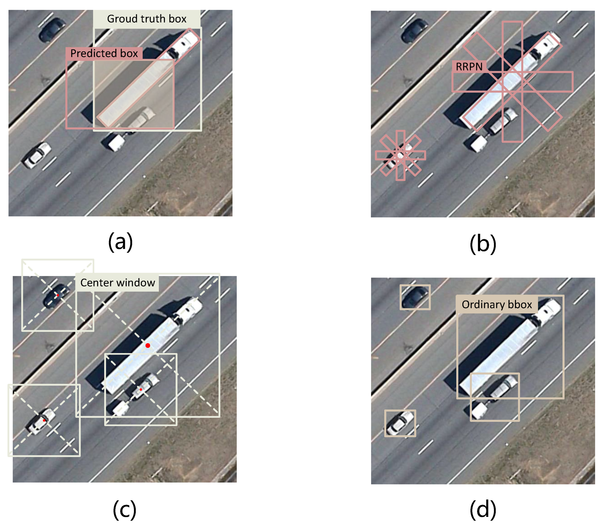
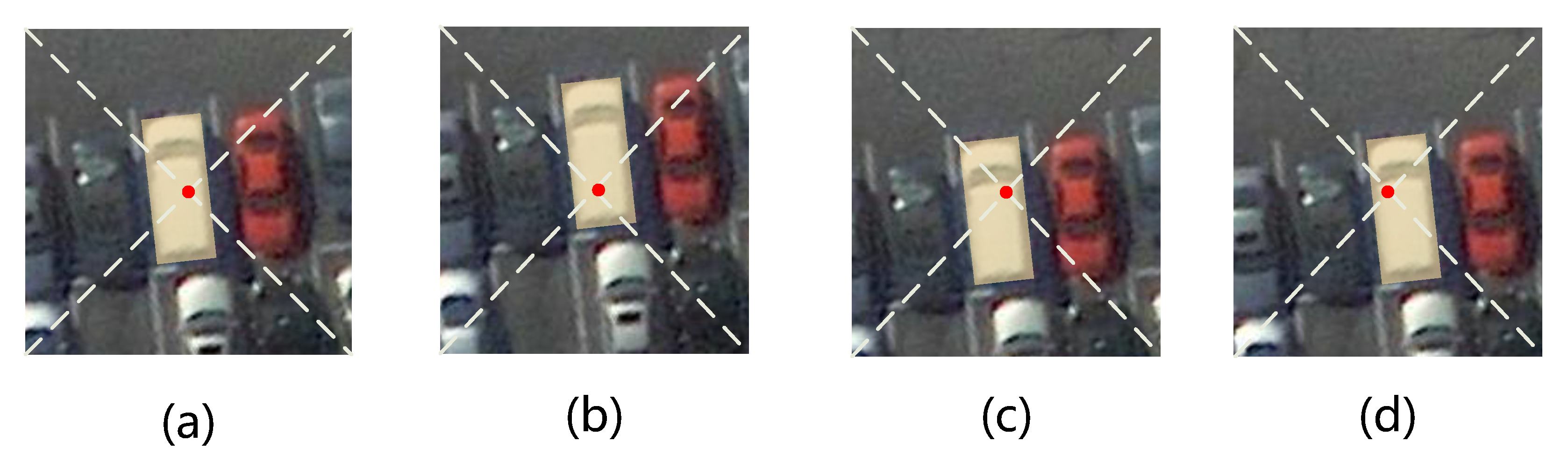
1. Introduction

Vehicle detection plays a significant role in optics remote sensing (RS) imagery interpretation, supporting numerous downstream applications, e.g., surveillance, defense, traffic planning, etc. [1,2,3,4,5]. However, vehicle detection is an extremely challenging task because vehicles are usually small with varied appearances and directions, and are parked densely in many scenarios.

In the beginning, researchers used traditional methods for vehicle detection in remote sensing images. These conventional methods mainly utilized low-level features and some manual features designed with prior human knowledge. These features include a histogram of oriented gradients (HOG) [6], scale-invariant feature transform (SIFT) [7], color histogram, texture feature, etc. Specifically, Shao et al. incorporate multiple visual features, a local binary pattern (LBP) [8], HOG, and an opponent histogram for vehicle detection in high-resolution RS images. Moranduzzo et al. [9] first use SIFT to detect interest points of vehicles, and then train a support vector machine (SVM) to classify these interest points into the vehicle target or not into the vehicle target. They later present an approach [10] that performs filtering operations in horizontal and vertical directions to extract HOG features and yields vehicle detection after the computation of a similarity measure, using a catalog of vehicles as a reference. Liu and Mattyus [11] used the AdaBoost classifier and similar Haar features to achieve a more robust and fast vehicle detection. Besides, ElMikaty et al. [12] use a sliding window framework consisting of four stages, namely, window evaluation; the extraction and encoding of features; classification; and post-processing, to detect cars in complex urban environments by using a combined feature of the local distributions of gradients, colors, and texture. In addition, Zhou et al. [13] rotate the sliding window and then classify the rotated sliding window to accomplish vehicle detection in any direction, but the detection speed of this method is relatively slow. Later, Kalantar et al. [14] utilize a region-matching approach to detect vehicles in remote sensing video frames captured by UAVs.

For almost a decade, neural networks have been experiencing a Renaissance, since Alexnet [15] won an image classification contest in 2012. Subsequently, ZFnet [16], VGGnet [16], and Resnet [17] appeared one after another, and the convolutional neural network (CNN) keeps refreshing the records of the classification task [18,19,20]. Ross and Kaiming introduce CNN into the detection task and propose a series of effective algorithms, such as R-CNN [21], Fast R-CNN [22], Faster R-CNN [23], and an improved detector based on Faster R-CNN [24,25,26], whose results reach an unprecedented high level.

Of course, the above methods also promote the development of RS vehicle detection. Recently, a series of advanced vehicle detectors [27,28] place more emphasis on how to output high-quality rotated bounding boxes due to the flexible representation. Among these methods, detectors based on anchor and regression occupy the mainstream, and offer the representation of multi-oriented vehicles by a rotated bounding box (bbox) or quadrangles. Although these oriented detectors have achieved promising results, they still suffer from some fundamental problems. Specifically, in the anchor-based detector, if the vehicle has a large aspect ratio, some issues, as shown in Figure 1a, may occur when the anchor matches with the ground truth (GT). The intersection-over-union (IoU) between a detected predicted box and the ground truth box is large enough. However, it is unreasonable to define the detected predicted box as a positive sample, as it contains only a tiny amount of object information. If using this method to match the positive and negative samples, the performance and stability of the models will be seriously affected. RRPN [29] tries to solve this problem by introducing six angles for each generated anchor on the vanilla basis, as shown in Figure 1b. In this way, RRPN is more suitable for the oriented object detection task. However, it introduces multiple anchors, which leads to a large decrease in terms of speed. More seriously, these angle-guided distance-regression-based detectors suffer from two problems: (1) discontinuous regression values, which are directly caused by angular periodicity, and (2) the difficulty of regressing small vehicles. For small objects, even tiny regression deviations (height, width, or angle) can result in an object miss.

Accordingly, the accuracy of angle prediction is critical for vehicle detectors that use rotating bounding boxes. Small angular deviations can lead to severe (IoU) degradation, which, in turn, leads to inaccurate vehicle detection, especially in the case of vehicles with large aspect ratios. Some recent works try to solve these problems; for example, Yang et al. propose the IoU-smooth L1 loss [30], which eliminated the mutation of angular regression by adding boundary constraints. Later, they proposed the circular smooth label (CSL) [31] to change the angular regression problem to an angular classification problem in order to avoid the discontinuity of numerical regression. Based on this, they also proposed densely coded labels (DCL) [32] to use dense angle labels instead of CSL to speed up the angle classification branch. Zhou et al. [33] migrated the targets in the right-angle coordinate system to the polar coordinate system using two polar angles and one polar diameter to represent the targets. Wei et al. [27] modeled a remotely sensed target as two intersecting centerlines, and Chang et al. [34] modeled a remotely sensed target as nine on the target. These methods fundamentally solve the regression inaccuracy problem, but such methods are still not applicable due to the small and intensive nature of vehicle detection. Obviously, the above methods still employ the distance regression and still suffer from the problems mentioned above.

To fundamentally avoid distance regression and considering the above shortcomings of current models in the vehicle detection task, in this paper, we propose a novel vehicle instance modeling method that regards each vehicle box as a saliency area. Based on the new representation, we propose SR-Net, which transforms the vehicle detection task into a saliency object detection task. This design, without any distance regression, allows our model to fundamentally avoid the aforementioned problems. Specifically, we first introduce the concept of the center window for each vehicle object. We define the center window as a square region and the vehicle’s center point as the center point of the center window. We divide the center window into two sizes, i.e., large and small. As shown in Figure 1c, we define all pixels in the oriented vehicle box located in the center of the center window as the saliency area (salient object). It is worth noting that our saliency region is very different from binary segmentation, as shown in Figure 2. Besides, we design two networks to estimate both the center window and the saliency area. We make the center window detection network focus on global information to estimate all center windows and make the saliency region detection network only focus on local information to better predict the saliency area. The overall flow of our approach is shown in the Figure 3. To obtain a more robust saliency region in the training stage, we add supervision to each side path of the saliency region estimator network. Finally, an edge capture module is devised to enhance the boundary information in order to obtain a more accurate saliency region boundary. In the inference stage, we only take the maximum value on the heatmap of the center window detection network as the target center window to avoid the post-processing of complex rotating non-maximum suppression (NMS). Experiments show that the oriented boxes decoded by the saliency region output by our SR-Net are more accurate. They do not suffer from the problems of inaccurate and discontinuous angular regression, as shown in Figure 4. In summary, the main contributions of this paper are four-fold.

• We propose a new model, SR-Net, to exploit saliency-area-based representation and localize the vehicle objects in remote sensing images. To the best of our knowledge, we are the first to detect vehicles via saliency object detection;
• Our model can handle the discontinuous problem of angular regression by replacing vanilla oriented-box-based representation with the proposed distance-regression-free saliency-area-based representation;
• To obtain a more accurate boundary of the saliency region and enhance the edge information of the saliency area, we design a contour-aware module to capture the object’s edge;
• To eliminate the divergence of feature construction, we propose a new pipeline that divides the localization networks and saliency-based representation networks into two paths.

Extensive ablation studies are conducted to verify the effectiveness of our developments. Specifically, our method is compared with state-of-the-art (SOTA) methods and achieves a competitive performance in vehicle detection. Specifically, for the DOTA, UCAS-AOD, DLR $3K$ Munich, and VEDAI datasets, the average AP boosting of our model is 2.32 compared to the SOTA.

In the rest of the article, the method is described in detail in Section 1. Then, we conducted experiments to compare with some of the state-of-the-art methods in Section 2. Section 3 presents the ablation study, analysis, and discussion. Finally, Section 4 provides a summary of our approach and an outlook for future work.

2. Method

We first provide an overview of the approach. As shown in Figure 5, SR-Net consists of two modules, namely, the center window estimator module and the saliency region detection module. We first generated the center window on the center window estimator pipeline. With all of the center windows, we then introduced a saliency region detection algorithm to pursue a high-quality representation of the vehicle and decoded final predicted bboxes. In this section, we first introduce the detailed structure of the center window estimator module and the design of loss functions. Then, the saliency region detection module and edge capture module are introduced to generate the saliency region with high precision.

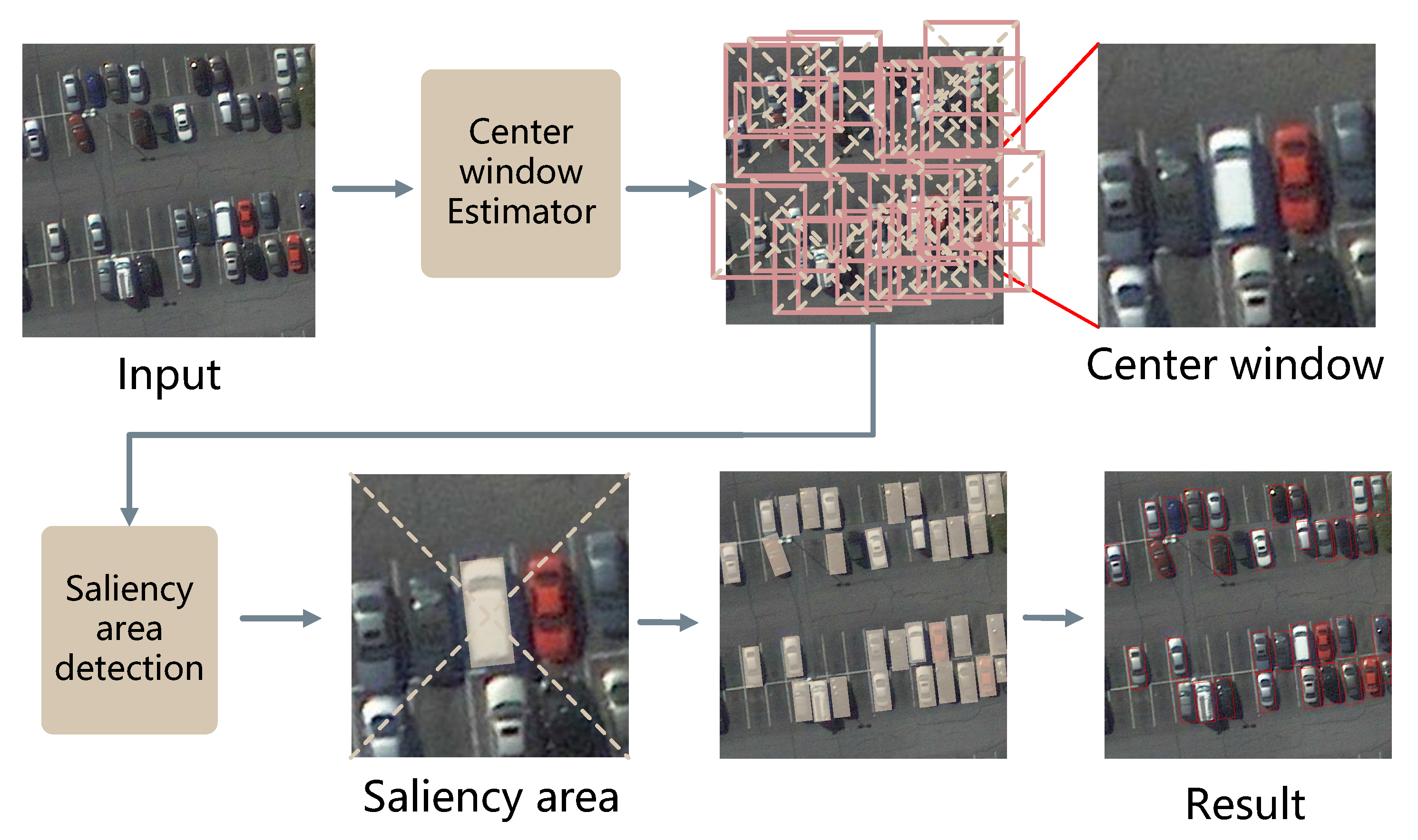
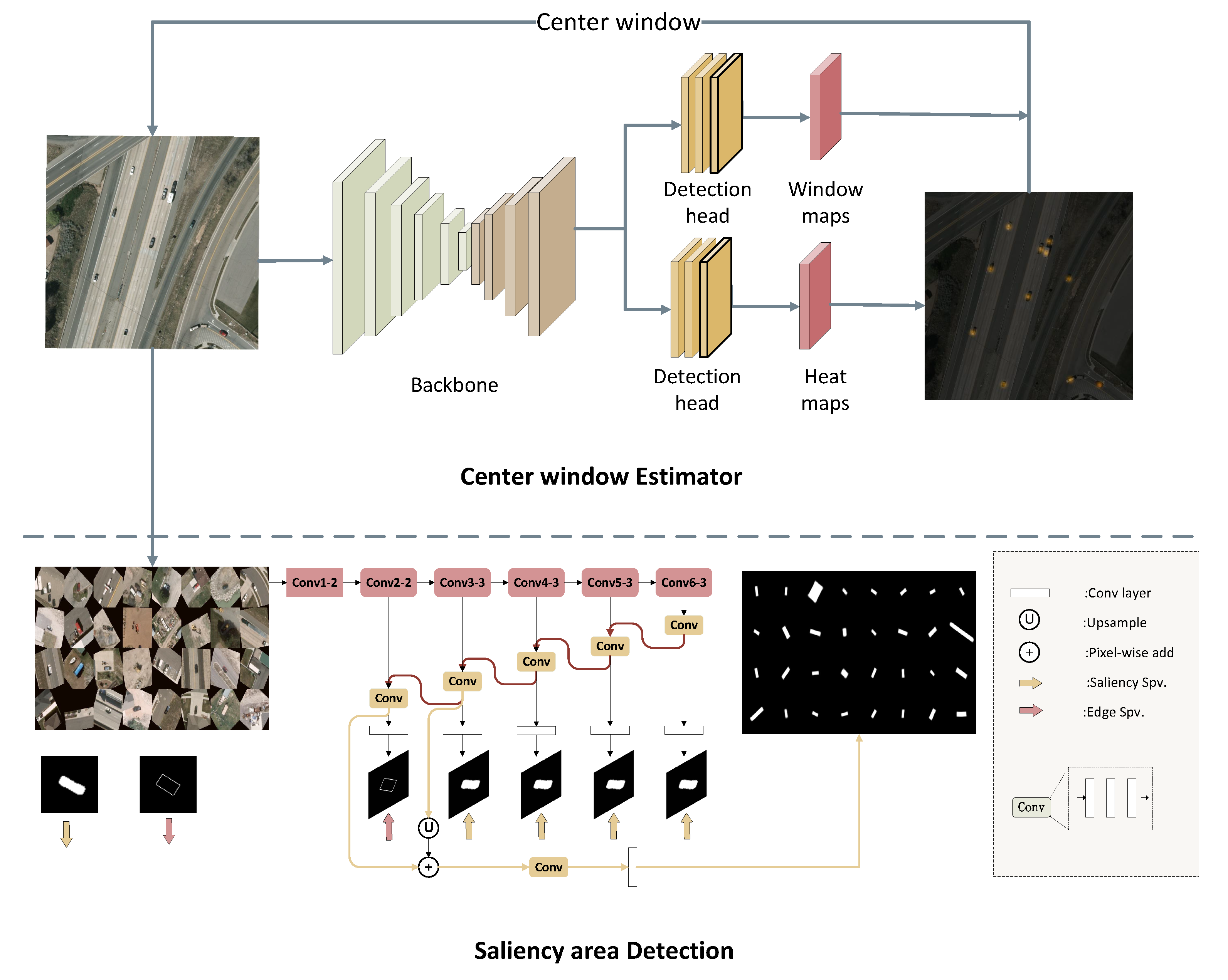
2.1. Center Window Estimator Module

In the center window estimator network, a vehicle is defined as a center point with a fixed-size window. We used the convolutional neural network (CNN) to predict a series of heat maps to represent the center of the vehicle. Meanwhile, the network also predicts the window size (large or small) corresponding to the center of the vehicle and slightly adjusts the position of the center point by predicting the offset. Upon the predicted vehicle center point, center window category, and offset, we adopted simple post-processing to obtain the corresponding center window of each vehicle. Figure 5 provides an overview of the center window estimator network. An hourglass network [35] was used as the backbone network, followed by a prediction module. Unlike other detectors, we did not use features from different scales to solve the scale discrepancy problem.

2.1.1. Center Window Estimator

As shown in Figure 5, we refer to the design of Center-Net [36]. The center window estimator network is a pure convolutional network, and an hourglass network [35] that introduces introducing channel attention was adopted as the backbone network for the center point estimator. The detection head consists of two prediction modules to predict the center point of each vehicle, and the category of the center window. Each prediction head consists of three layers of convolution. The first two convolution layers use the ReLU activation function, and the three convolution layers use convolution kernels of sizes 3 × 3 × 128, 3 × 3 × 128, and 1 × 1 × 1. Here, the last channel means that there is only one output category of SR-Net, i.e., vehicles. In the last output layer, the sigmoid function was selected for activation in order to map output values to the range of 0 to 1, as shown in Figure 6.

2.1.2. Center Estimator Loss Function

Heat map channels were used to predict central points, among which is a binary mask indicating the locations of the center for an object. For each center, there is one ground truth positive location, and all other locations are negative. In the training process, not all negative positions are equivalently penalized, but the penalty for negative positions within the radius of the positive position is reduced.

The false center detections that are close to the ground truth locations can still produce the locating centers accurately. Specifically, the radius depends on the size of the vehicle, and the points within the radius are ensured at least inside the target ground truth bbox. Meanwhile, the extent of penalty reduction is given by an un-normalized 2D Gaussian according to the radius, $e^{\frac{x^2+y^2}{2{\sigma }^2}}$, in which, ${\sigma }^2$ is 1/2 of the radius. $p_{ij}$ is denoted as the score at location $(i,j)$ for object in the predicted heatmaps and $y_{ij}$ is denoted as the “groundtruth” heatmap augmented with the unnormalized Gaussians. Based on the above analysis, we designed a variation of focal loss:

$$L_{det}=\frac{1}{N}\sum _{i=1}^H\sum _{j=1}^W\left\{\begin{array}{c}{(1-p_{ij})}^{\alpha }log(p_{ij})if{y}_{ij}=1\\ {(1-y_{ij})}^{\beta }{(p_{ij})}^{\alpha }log(1-p_{ij})otherwise\end{array}\right.$$

(1)

where N denotes the number of vehicles in the current image, $\alpha$ is the hyperparameter that controls the weight of difficult samples, and $\beta$ is the hyperparameter that controls the imbalance between positive and negative samples. We set $\alpha$ to 2 and $\beta$ to 3 in all experiments. The ($1-y_{ij}$) term reduces the penalty around the ground truth locations with the Gaussian bumps encoded in $y_{ij}$. Downsampling layers are involved in our networks to gather global information and reduce memory consumption. The size of the output is usually smaller than the image when fully convolutionally applying them to an image. Therefore, the position in the original image $(x,y)$ corresponds to the position in the heat map $({\displaystyle \frac{x}{n}},{\displaystyle \frac{y}{n}})$, where n is the coefficient of downsampling of the heat map with respect to the original image. Some precision may have been lost when we remapped the locations from the heatmaps to the input image, which can seriously affect the center-locating accuracy of small vehicles. To solve this problem, we predicted the offset of the centroid position and slightly adjusted the centroid position before generating the center window based on the centroid.

$$o_k=(\frac{x_k}{n}-[\frac{x_k}{n}],\frac{y_k}{n}-[\frac{y_k}{n}])$$

(2)

where $o_k$ is the offset and $x_k$ and $y_k$ are the x and y coordinates for center k. Particularly, we predicted a set of offsets shared by the centers of all categories. In the training stage, the $smoot{h}_{L1}$ loss (Girshick, 2015) was applied at the ground truth center locations:

$$L_{off}=\frac{1}{N}\sum _{k=1}^{N}Smoot{h}_{L1}(o_k,\stackrel{}{{\widehat{o}}_k})$$

(3)

2.1.3. Center Window

Different from other networks, after we obtained the center point of each vehicle, we did not directly regress the length, width, and angle of the vehicle We predicted a vehicle size category (large and small) for the center point of each vehicle. The unique center window was jointly determined by the the center point and size of each vehicle. In this way, we ensured that the vehicle was not only inside the center window but also in the center of the center window. Our central window category prediction head was also composed of three convolutional layers, with convolutional kernels of size $3\times 3\times 128$, $3\times 3\times 128$, and $1\times 1\times 2$ in each convolutional layer. Here, the last channel implies the classification result. In the final output layer, we used the softmax function to activate it. For training, we applied the crossentropy loss.

$$L_{class}(p_i,c_i)=\frac{1}{N}\sum _{i=1}^{i=N}\left\{\begin{array}{c}-log(p_i(c_i))if{c}_i=large\\ -\delta log(p_i(c_i))else\end{array}\right.$$

(4)

where $\delta$ is a parameter used to balance the imbalance of the size vehicle data. We set it to 0.3 In the center window estimator stage, our loss function could be expressed as:

$$L_{CE}=\gamma L_{class}+(L_{off}+L_{det})$$

(5)

where $L_{CE}$ denotes the total loss in the center window estimator stage, and $\gamma$ is the coefficient.

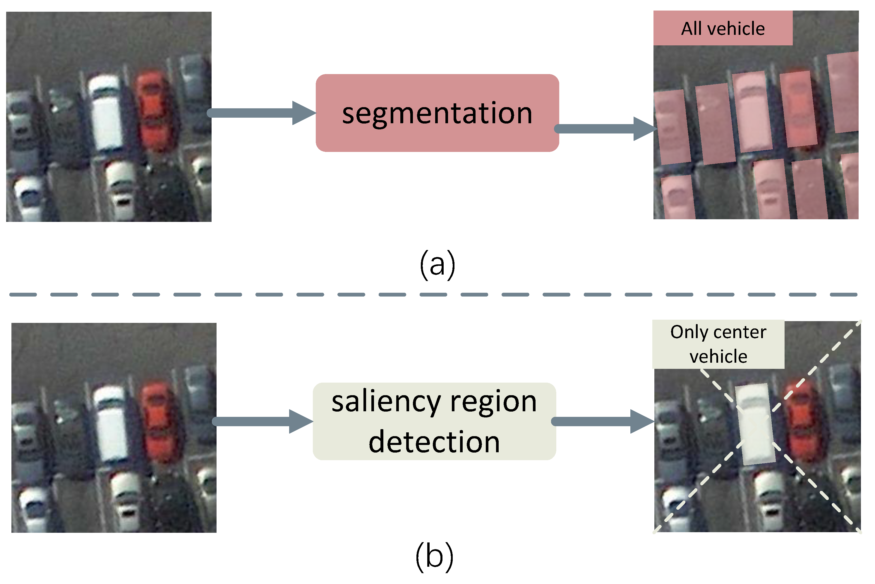
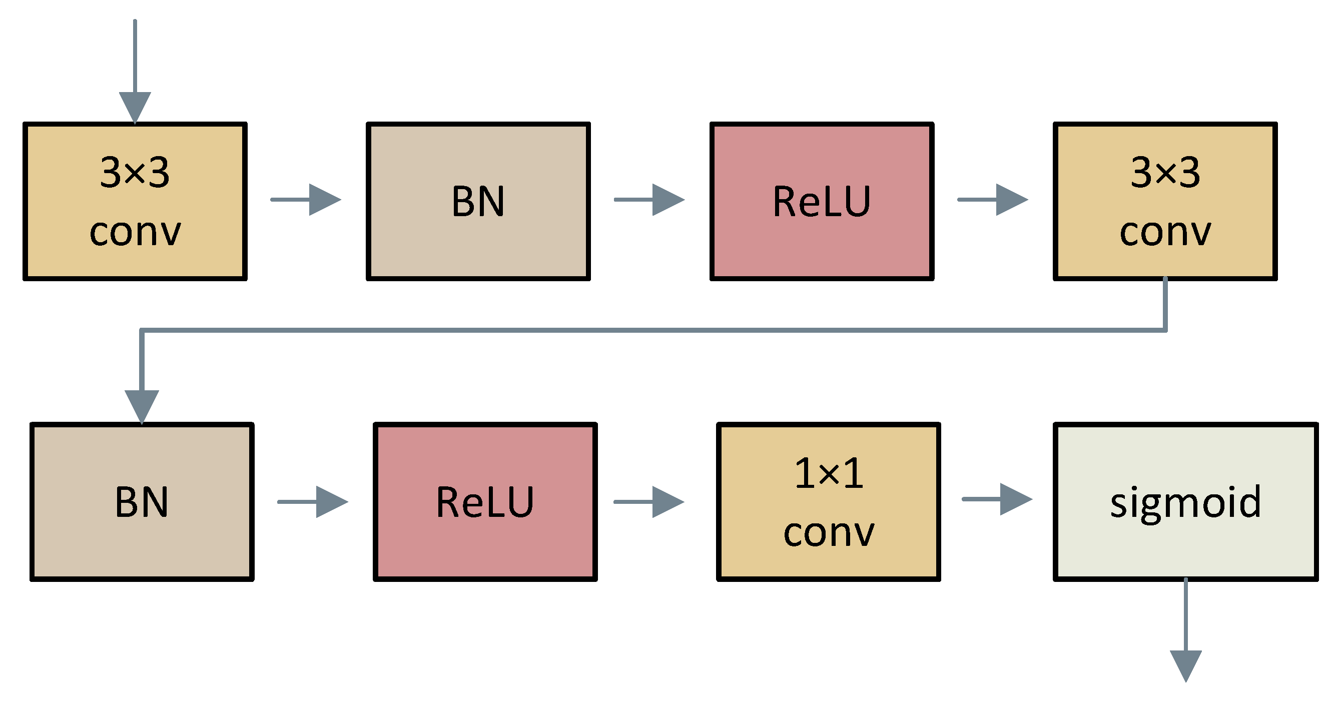
2.2. Saliency Region Detection

The role of the saliency region detection network is to accurately represent a coarse representation of the vehicle (center window) as an accurate representation at the pixel level. The design of our saliency region detection network took into account some existing saliency detection models [37,38,39]. In the saliency region detection network, we cut the center window on the input image according to the center window generated by the center window estimator network. For each center window area, we used the saliency region detection network to detect its saliency region, which is defined as the central object in this area. The specific structure of our saliency region detection network is shown in Figure 5. The effect is shown in Figure 7. In the saliency region detection network, we obtained five features with high resolution and rich semantic information through multi-level feature fusion. We supervised each feature map, where four of them were used to obtain the region of significance and the other to obtain the edge of the area. Finally, we fused the results from the edge capture module’s features and the saliency region detection module’s features and obtained a accurate saliency detection.

2.2.1. Complementary Information Modeling

Our proposed network architecture is independent of the feature extraction backbone; here, the architecture is based on VGGNet, like many previous CNN-based methods. The architecture we proposed can be found in the saliency region detection part of Figure 5. Following DSS, we discarded the full connection layer in the original network. Six features called Conv1-2, Conv2-2, Conv3-3, Conv4-3, Conv5-3, and Conv6-3 were generated from VGGNet; we denoted them as $C^{(1)}$, $C^{(2)}$, $C^{(3)}$, $C^{(4)}$, $C^{(5)}$, and $C^{(6)}$ for simplicity. Then, we used side paths to obtain corresponding side outputs, except $C^{(1)}$, because the number of convolutional layers spaced between $C^{(1)}$ and the inputs was too low and the perceptual field was too small. Five side paths are denoted by a path set S:

$$S=\left\{S^{(2)}\right.,S^{(3)},S^{(4)},S^{(5)},\left.S^{(6)}\right\}$$

(6)

Conv2-2 has the highest resolution of these features while retaining the complete edge information due to its proximity to the input. We leveraged $S^{(2)}$ to obtain edge output and other outputs to obtain saliency object output in the later network.

2.2.2. Saliency Object Features Extraction

In order to leverage rich semantic and high-resolution information in multi-level side outputs, we imitated widely used architecture U-Net [35] for feature fusion. Different from the original U-Net [35], we added three extra convolutional and ReLU layers (orange Conv block in Figure 5) on each side path to obtain more robust fused features. For simplicity, we used H (

Table 1. The detailed convolutional structure of the prediction head. H denotes the feature enhancement module in each prediction header, each prediction header contains three convolutional layers—$H_1$, $H_2$, $H_3$—and each convolutional layer is followed by a ReLu activation function. The table shows the parameters of each convolutional layer; for example, 3, 1, 64 indicates a convolutional layer with convolutional kernel size of 3, padding of 1, and channel number of 64. O represents the output layer, which transforms the multi-channel features into a single-channel activation map.

S	${\mathit{H}}_1$			${\mathit{H}}_2$			${\mathit{H}}_3$			O
2	3	1	64	3	1	64	3	1	64	3	1	1
3	3	1	128	3	1	128	3	1	128	3	1	1
4	3	1	256	3	1	256	3	2	256	3	1	1
5	5	2	256	5	2	256	5	2	256	3	1	1
6	5	2	256	5	2	256	5	2	256	3	1	1

) to denote these convolutional layers and ReLU layers in the side path. Then, we used a convolutional layer which was denoted as O (Table 1) to transit the feature maps to the single-channel prediction masks. The details of convolutional layers in the side path can be found in Table 1.

2.2.3. Saliency Edge and Region Masks Extraction

In this section, our aim is to model the saliency edge information while obtaining saliency edge features. As mentioned in the previous section, Conv2-2 has the highest resolution and retains the most complete edge information. Therefore, our local edge information was extracted from Conv2-2. However, saliency edge features cannot be obtained with only local edge information. We also needed high-level semantic information. When the semantic information at the top layer is passed back to the bottom layer from the top layer, like the U-Net structure, the semantic information at the top layer will be diluted. Therefore, we designed top-down layer-by-layer information propagation, in which, supervision is added at each layer.

Our high-level semantic information was propagated to the side path $S^{(2)}$ via a top-down path to suppress non-saliency edges. The fused saliency edge features $C_E$ can be expressed as:

$$C_E=C^{(2)}+U(ReLU(Conv({\widehat{\Lambda }}^{(6)};\phi ));C^{(2)})$$

(7)

where $Conv(\ast ;\phi )$ is a convolutional layer with trainable weight $\phi$ and a convolutional kernel size of $1\ast 1$. It was intended to have the same number of channels for the features. The $ReLU$ denotes the $ReLU$ activation function and $U(\ast ;C^{(2)})$ denotes the size of the * upsampled to $C^{(2)}$ resolution (using a bilinear interpolation method). ${\widehat{\Lambda }}^{(6)}$ is the fused feature in the side path. ${\widehat{\Lambda }}^{(6)}$ can be denoted as $\mathrm{E}(C^{(6)};W_T^{(6)})$ and the fused feature ${\widehat{\Lambda }}^{(3)}$, ${\widehat{\Lambda }}^{(4)}$, ${\widehat{\Lambda }}^{(5)}$ in the same side paths $S^3$, $S^4$, $S^5$ can be denoted as

$${\widehat{\Lambda }}^{(i)}=\mathrm{E}(C^{(i)}+U(ReLU(Conv({\widehat{\Lambda }}^{(i+1)};\theta ));W_H^{(i)})$$

(8)

where $\mathrm{E}(\ast ;W_H^{(i)})$ denotes the convolution layer and activation function with parameters $W_H^{(i)}$. Saliency edge features $F_E$ in $S^{(2)}$ could be computed as $\mathrm{E}({\overline{C}}^{(2)};W_H^{(2)})$. The configuration details could be found in Table 1. We supervised the saliency edge and the saliency region prediction maps, respectively. For saliency edge supervision, we used the cross-entropy loss, which could be defined as:

$$\begin{array}{c}{L}_{edge}(F_E;W_O^{(2)})=-{\displaystyle \sum _{j\in G_{+}}}log{P}_r(y_i=1|F_E;W_O^{(2)})-\hfill \\ {\displaystyle \sum _{j\in G_{-}}}log{P}_r(y_i=0|F_E;W_O^{(2)})\hfill \end{array}$$

(9)

where $G_{+}$ and $G_{-}$ denote the pixels in the saliency edge and the pixels in the background region, respectively. $W_O$ denotes the parameters of the prediction layer, as shown in Table 1, and $P_r(y_i=1|F_E;W_O^{(2)})$ denotes the confidence level that the pixel has a saliency edge. In addition, for saliency region supervision, we used the cross-entropy loss, which could be defined as:

$$\begin{array}{c}{L}_{area}({\widehat{\Lambda }}^{(i)};W_O^{(i)})=-{\displaystyle \sum _{j\in A_{+}}}log{P}_r(y_i=1|{\widehat{\Lambda }}^{(i)};W_O^{(i)})-\hfill \\ {\displaystyle \sum _{j\in A_{-}}}log{P}_r(y_i=0|{\widehat{\Lambda }}^{(i)};W_O^{(i)})\hfill \end{array}$$

(10)

where $A_{+}$ and $A_{-}$ denote the pixels in the saliency region and the pixels in the background area, respectively. The total relay supervision $L_{Relay}$ can be expressed as:

$$L_{Relay}=L_{edge}(F_E;W_O^{(2)})+\sum _{i=3}^6{L}_{area}({\widehat{\Lambda }}^{(i)};W_O^{(i)})$$

(11)

2.2.4. Saliency Object Detection

After obtaining the saliency edge and saliency areas outputs, our goal is to use edge output to obtain better segmentation results. Then, we can obtain the detection boxes by calculating the minimum external rectangle of these segmentation results. Specifically, we fused $F_E$ with edge features and ${\widehat{F}}^{(3)}$ with regional features to obtain the complete feature $F_W$.

$$F_W={\widehat{F}}^{(3)}+Up(ReLU(Conv({\widehat{F}}^{(3)};\theta ));F_E)$$

(12)

We also supervised the final predicted saliency region, with the loss function expressed as the following equation.

$$\begin{array}{c}{L}_{Saliency}(F_W;W_E^{})=-{\displaystyle \sum _{j\in Y_{+}}}log{P}_r(y_i=1|F_W;W_E^{})-\hfill \\ {\displaystyle \sum _{j\in Y_{-}}}log{P}_r(y_i=0|F_W;W_E^{})\hfill \end{array}$$

(13)

The supervision losses of all parts were combined as follows:

$$L_t=\eta L_{Relay}+L_{Saliency}$$

(14)

where $\eta$ denotes the weight of the relay supervision loss to the total loss, and the effect of $\eta$ on the final result is discussed in the next section.

3. Result

In this section, we conduct experiments to evaluate the performance of SR-Net. First, we introduce some training details of SR-Net, such as dataset, hyperparameters, etc. Then, we introduce the evaluation metrics. Finally, we present the ablation experiments with some parameters and structures of our SR-Net and compare them with current state-of-the-art detectors to derive the effectiveness of our method.

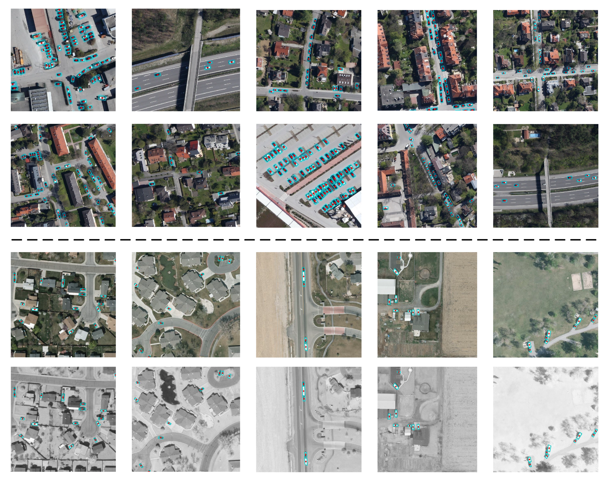
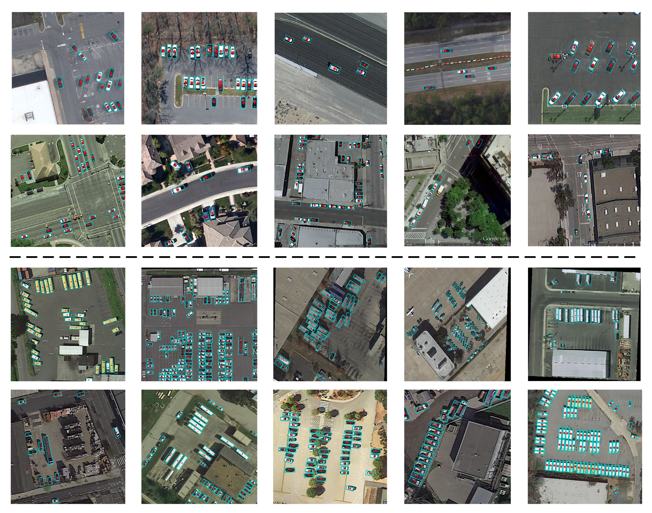
3.1. Data Set

(1) DOTA [40]: DOTA is a standard benchmark for the detection of objects in remote sensing images.It contains two detection tasks: detection with oriented bounding boxes and detection with horizontal bounding boxes. Only detection with oriented bounding boxes is used in our experiments. The DOTA contains 2806 remote sensing images. DOTA is labelled with 15 categories (e.g., aircraft, small vehicle, large vehicle), and, in this paper, we only use two categories: small vehicles and large vehicles. In training, we crop the large-scale images in DOTA into multi-scale remote sensing image slices of size 384 × 384, 512 × 512, and 800 × 800.

(2) UCAS-AOD [41]: The UCAS-AOD dataset contains 510 large-scale remote sensing images with two types of targets (aircraft and vehicles) in the UCAS-AOD dataset containing 7114 vehicle targets. We randomly select 400 images for training and the other images for testing. Similarly, we slice the large-scale remote sensing images to obtain multi-scale slices of size 384 × 384, 512 × 512, and 800 × 800 for training.

(3) DLR 3K Munich [11]: In the DLR 3K Munich, vehicles are accurately labeled by rotatable rectangular boxes. This dataset consists of three categories (car, bus, and truck), and we consider the three categories as one class.The dataset contains a total of 8268 vehicles, of which, the training set contains 5214 vehicles and the test set contains 3054 vehicles.

(4) VEDAI [42]: VEDAI contains two modal images, RGB and NIR, and four classes (car, pickup, truck, van), which, again, we still consider as one class. The dataset contains a total of 5494 vehicles, with a training set of 2792 and a test set of 2702.

3.2. Evaluation Metric

In the detection task, the output of the model can be represented as a rotatable rectangular bounding boxes and its corresponding class. For our vehicle detection, since we use single-category detection, our output is only rotatable rectangular bounding boxes. We evaluate the accuracy of the detected boxes by using the intersection over union (IoU) metric. The IoU denotes the number of detected boxes and the overlap rate between detected boxes and ground truth boxes. The formula for IoU is defined as:

$$IOU=(S_{bbox}\cap S_{gt})/(S_{bbox}\cup S_{gt})$$

(15)

where $S_{box}$ denotes the region of the detection box and $S_{gt}$ denotes the region of the ground truth box. We use average precision $(AP)$ to evaluate the merit of the vehicle detection method. In order to calculate the AP value, we need to define and calculate the following values based on the detection results true positives $(TPs)$, false positives $(FPs)$, true negatives $(TNs)$, and false negatives $(FNs)$.

In our vehicle detection task, we set the threshold of IoU between the detection box and the ground truth box. If the IoU between a detection box and ground truth box is greater than the threshold, this detection box is considered as $TP$. Conversely, if the $IoU$ is less than the threshold, this detection box is considered $FP$ (also called false alarm). If a ground truth box is not detected, this ground truth box is called $FN$ (also called miss alarm). Based on the above definition, we define the equation of the precision and recall metrics as:

$$Precision=\frac{TP}{(TP+FP)}$$

(16)

$$Recall=\frac{TP}{(TP+FN)}$$

(17)

The AP is calculated by integrating the $P(Precision)$-$R(Recall)$ curve. The P-R curve can be obtained by calculating the recall values corresponding to different precision values based on the detection results. Based on this definition, it is known that, the higher the AP value, the better the performance of the model. The AP value can be defined as:

$$AP=\underset{0}{\overset{1}{\int }}P(R)d(R)$$

(18)

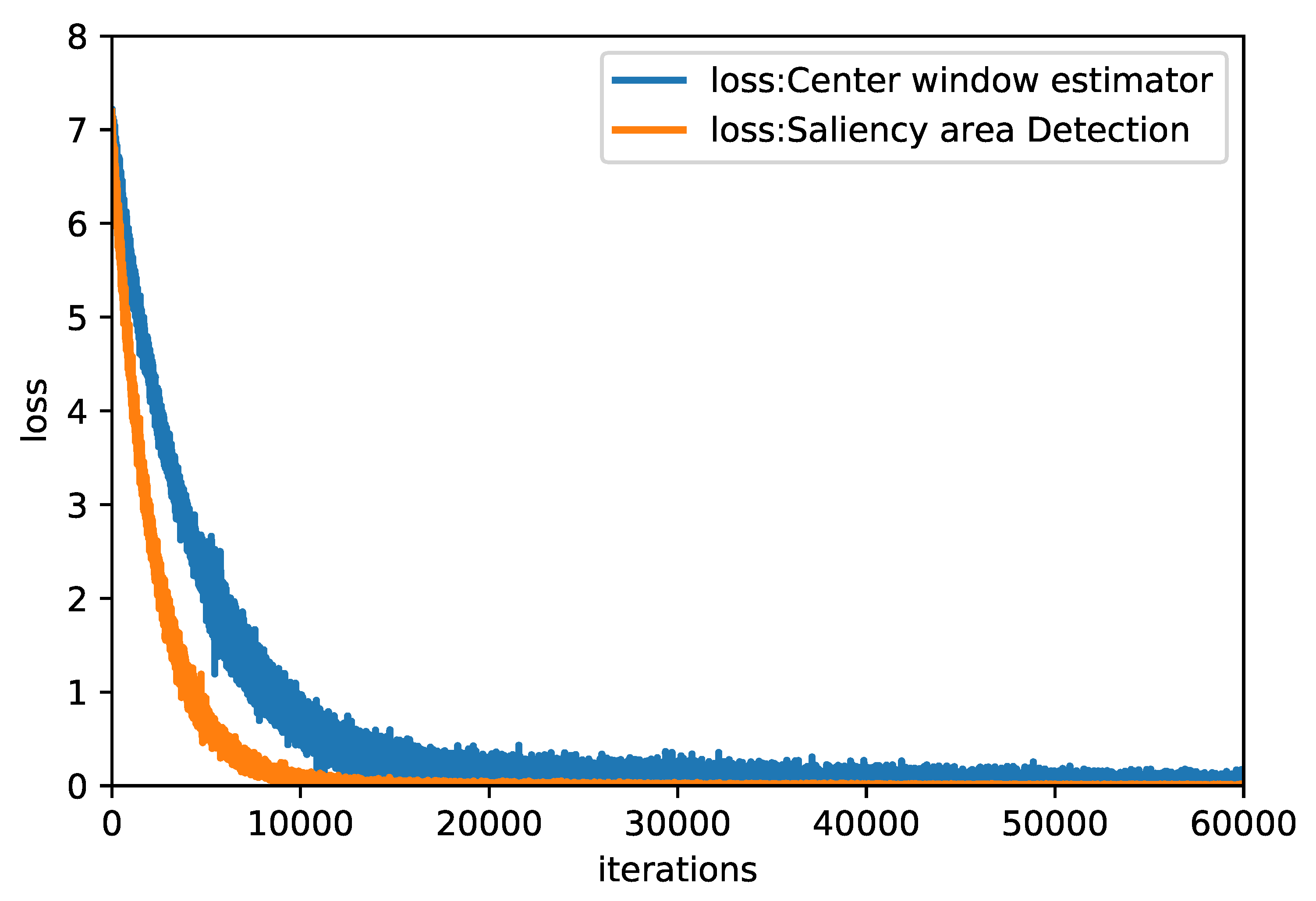
3.3. Training Details

We implement SR-Net in PyTorch (Paszke et al., 2017). During the center window forecasting phase, our center window estimator section is trained on an image with an input resolution of 512 × 512, corresponding to our output of a heat map with a resolution of 128 × 128. To ensure a diversity of vehicle sizes, our training set was produced with multiple scales (384 × 384, 512 × 512, and 800 × 800), so we uniformly resized it to a 512 × 512 size using bilinear interpolation, which, in addition, enhanced the robustness of the model and reduced the risk of overfitting. We also used data enhancement methods, such as rotation, color transformation, etc. Finally, Adam [43] was used to optimize the overall objective.

We train our SR-Net with a batch-size of 32 (on two GPUs), and we train the model from scratch to 60,000 iterations in order to achieve the best results. The convergence curve of the model is shown in Figure 8. During the saliency region detection phase, since the data are labeled in the form of rotating boxes, which do not meet the supervision information required, we first need to generate the center window for each vehicle based on the definition of our saliency area. We need to transform the rotating frame annotation into a pixel-level segmentation annotation by defining the pixels in the target region as saliency areas. To enhance stability enhancements were also made as shown in Figure 9. In order to train our edge information enhancement module, we need to label the saliency region to extract the edges using the edge extraction operator (we use the Canny operator). During training, we resize each center window to a uniform size of 32 × 32. Again, to ensure sample diversity and eliminate the risk of overfitting, we use the same data enhancement as in the center window estimator stage. Again, we use Adam to optimize the parameters. In this stage, we only need 10,000 iterations to obtain the best results.

3.4. Comparisons with State-of-the-Art Detectors

In this section, we compare SR-Net with other state-of-the-art detectors. We evaluate our model and other models in a vehicle detection task on four datasets. For SR-Net, we use two backbone networks (104-Hourglass, ResNet-101). For the other models, we follow the authors’ previous backbone networks. We also test the difference in inference speed between our model and the other models to verify the advantages of our model. The detection results of our model on DLR 3K Munich and VEDAI datasets are shown in Figure 10, and the test results on DOTA and UCAS-AOD are shown in Figure 11. In addition, to verify the generalization ability of our model, we trained our SR-Net on the ensemble of four datasets and tested our model on a panoramic map of a residential region from Google Maps. The results are shown in Figure 12.

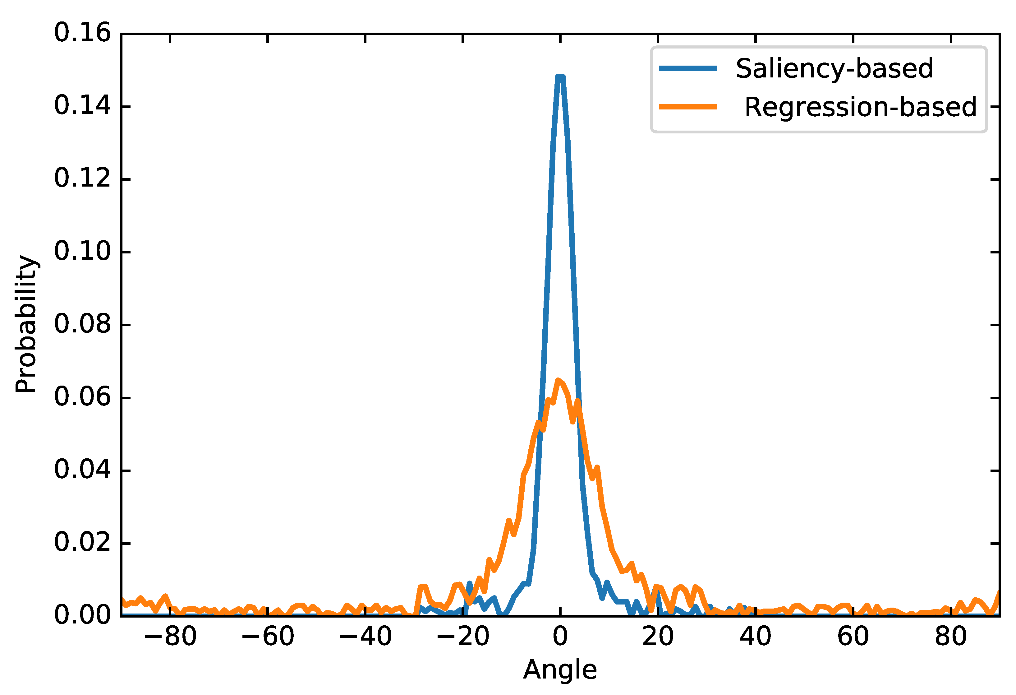
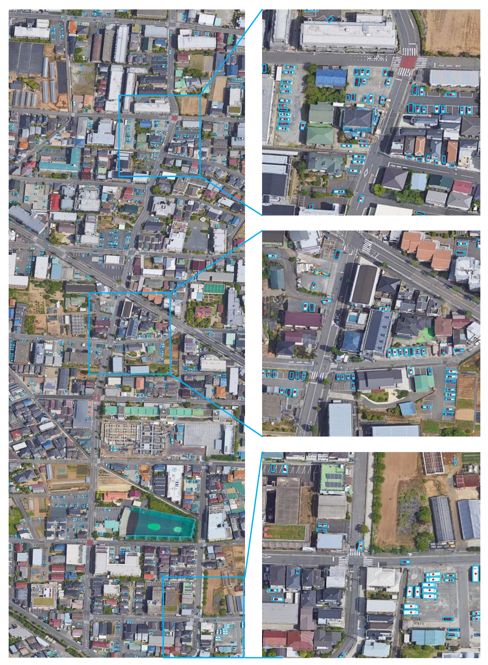
3.5. Qualitative Quantity Analysis

As shown in

Table 2. State-of-the-art comparisons. AP is the average of 10 values of AP taken between $iou=50$ and $iou=95$. AP${}^1$ denotes the AP value obtained in the DOTA validation set, AP${}^2$ denotes the AP value obtained in the UCAS-AOD test set, AP${}^3$ denotes the AP value obtained in the DLR 3K Munich dataset test set, and AP${}^4$ denotes the AP value obtained in the VEDAI test set. AP${}^m$ denotes the average of the AP values obtained in the four datasets. AP${}_{50}$ is the AP value obtained in the $IoU=50$, and AP${}_{75}$ is the AP value obtained at $IoU=75$.

Models	FPS	AP${}^1$	AP${}_{50}^1$	AP${}_{75}^1$	AP${}^2$	AP${}_{50}^2$	AP${}_{75}^2$	AP${}^3$	AP${}_{50}^3$	AP${}_{75}^3$	AP${}^4$	AP${}_{50}^4$	AP${}_{75}^4$	AP ${}^{\mathit{m}}$
YOLOv2(O) [44]	15.31	4.43	6.70	4.73	11.29	18.21	12.74	12.84	20.32	14.30	12.25	19.80	14.36	10.20
$R^{2}CNN$ [45]	3.81	34.94	57.20	41.64	59.83	87.95	61.88	59.65	87.22	64.54	60.79	64.59	46.31	53.80
RRPN [29]	5.25	34.09	53.19	39.25	59.83	86.17	62.50	58.17	85.43	61.93	51.85	62.34	44.88	50.99
R-DFPN [46]	5.84	34.22	54.33	39.17	60.41	87.37	61.72	55.08	84.35	59.21	54.91	60.57	43.73	51.15
ICN [47]	6.54	45.64	65.77	48.20	58.24	89.24	64.93	54.34	86.12	63.81	56.15	63.22	44.94	53.59
RetinaNet(O) [25]	7.34	42.08	68.26	50.99	62.54	89.65	64.60	54.54	86.30	63.08	53.16	65.41	47.74	53.08
Roi-Transformer [48]	3.92	43.77	70.27	50.31	60.90	90.56	66.69	55.86	88.53	65.15	56.12	66.52	48.82	54.16
P-RSDet [33]	7.82	46.55	71.52	51.70	57.93	90.87	66.19	54.75	88.75	64.96	61.94	70.33	49.58	55.29
SCRDet [30]	6.37	40.17	65.97	47.56	57.27	90.25	64.40	56.58	89.67	63.21	55.77	74.65	54.34	52.44
$O^2$-DNet [28]	7.62	47.09	72.45	51.43	59.42	91.06	67.15	63.08	90.64	67.88	56.01	71.34	52.07	56.40
$R^3$-Net [49]	3.23	49.58	73.24	52.07	60.19	91.22	66.21	63.12	91.48	67.69	56.26	69.23	50.39	57.28
$R^3$-Det [50]	6.53	46.49	75.24	55.15	61.09	91.63	64.85	62.01	90.14	66.34	56.42	70.58	51.02	56.50
SR-Net(ResNet-101)	7.64	50.27	76.40	57.75	61.18	92.03	69.55	64.47	90.68	69.82	53.42	70.53	56.54	57.33
SR-Net(104-Hourglass)	7.43	52.30	80.09	59.03	62.44	93.24	70.55	68.25	91.01	71.89	55.81	72.53	58.16	59.60

, our proposed SR-Net achieved the highest results for AP values on the DOTA, UCAS-AOD, and DLR 3K Munich datasets, and AP${}^{75}$ still achieved the best results on the VEDAI dataset despite the fact that AP did not achieve the best results, again illustrating the advantages of our proposed method in terms of accuracy. The average results on the four datasets (AP${}^m$) showed an improvement of 2.32 compared to the previous method. In terms of speed, since we do not need rotational non-maximal suppression (RNMS), anchor, etc., our model achieves the highest AP value, while our speed is approximately twice that of $R^3$-Net.

4. Discussion

In this section, we perform detailed ablation experiments on the parameters and components of SR-Net. Besides, the advantages and disadvantages of the proposed method are discussed. All ablation experiments are performed using ResNet-101 as the backbone network and are trained and evaluated on the UCAS-AOD dataset.

Loss weight. We analyze the effect of the $\gamma$ parameter in Equation (5) on the SR-Net. As shown in

Table 3. The AP values of the results were obtained by comparing different $\gamma$ values on the UCAS-AOD dataset. (AP is the average of 10 values of AP taken between $IoU=50$ and $IoU=95$).

$\mathit{\gamma }$	0.1	1	2	3	5	7
AP	0.602	0.608	0.612	0.610	0.609	0.593

, the best results were achieved at a $\gamma$ value of 2. In addition, we found that a small selection of $\gamma$ values did not have a great impact on the final results. This indicates that the results of the center window prediction are more dependent on the accuracy of the center point prediction. It also shows that the network can easily predict the category of the center window. Similarly, we analyze the effect of the loss function of the relay supervision, i.e., the effect of the size of the parameter $\eta$ in Equation (14) on the final results. As shown in

Table 4. The AP values of the results were obtained by comparing different $\eta$ values on the UCAS-AOD dataset. (AP is the average of 10 values of AP taken between $IoU=50$ and $IoU=95$).

$\mathit{\eta }$	0	0.1	0.4	0.8	1.2	1.4	1.6
AP	0.574	0.586	0.604	0.609	0.612	0.610	0.608

, the best results are obtained when the value of t is 1.2, while it can be observed that the final result decreases significantly if no relay supervision is added, and that the final results are affected if the weight of relay supervision is too large.

Edge supervision. Since our method models vehicles at the pixel level, the accuracy of the saliency region edges directly affects the accuracy of the oriented bboxs generated from the saliency region decoding. In addition, in remote sensing images, the edges of vehicles are relatively clear, based on which, we design the edge supervision module to make the edges of saliency regions more precise. To verify the effectiveness of our edge supervision module, we perform ablation experiments. As shown in

Table 5. A comparison of the effect of adding edge supervision module and region supervision module on the results on UCAS-AOD dataset. (AP is the average of 10 values of AP taken between $IoU=50$ and $IoU=95$. AP${}_{50}$ is the AP value obtained in the $IoU=50$, and AP${}_{75}$ is the AP value obtained at $IoU=75$).

Edge Supervision	Area Supervision	AP	AP${}_{50}$	AP${}_{75}$
	✓	0.613	0.919	0.683
✓		0.612	0.942	0.695

, equipped with the area supervision module with the edge supervision module, the resulting AP value gains a 0.9% improvement, AP${}_{50}$ remains basically the same, and AP${}_{75}$ yields a 1.2% improvement, proving that the devised edge supervision can achieve finer boundaries.

Saliency-based. In this section, we will discuss the advantages of saliency-based over regression-based detection methods in detail. In the previous regression-based detection methods, the vehicle detection results are represented by the vehicle center, length, width, and angle, where length, width, and angle are obtained by distance regression. The objective function in distance regression is generally L1 loss, L2 loss, or a deformation based on them, and, in the distance regression, the network needs a clear objective value, yet, in the definition of an angle, it is periodic without a clear objective value, e.g., 0 degrees and 360 degrees. In the proposed saliency-based detection method, the detection result of the vehicle is represented by the center point of the vehicle and the corresponding saliency region. The saliency region is obtained by modeling the probability that each pixel belongs to the foreground, and modeling each pixel in the instance foreground is a binary classification problem, i.e., a logistic regression problem in which the loss function is the cross-entropy loss, as shown in Equation (14). Therefore, the saliency-based method does not have distance regression values in principle, and there is no problem with inaccurate regression values.

To further illustrate the problem, we compared the saliency-based method and the regression-based method through an experiment. In order to eliminate the influence of other components on the final results, we only compare the accuracy of the generated bbox. In particular, we obtain the labeled center directly in order to ensure the consistency of the vehicle center, assuming that all vehicle centroids are detected correctly. Then, for each vehicle centroid, regression is used to regress the vehicle’s length, width, and angle. Similarly, we use a saliency-based approach to generate the saliency region of the vehicle while keeping the centroids unchanged and decoding the vehicle’s aspect and angle based on the saliency area. For the angles of the oriented bboxes obtained by the two methods, we obtain Figure 4. This statistical plot clearly shows the angular error of oriented bboxes obtained by the two methods. The angle errors obtained by our saliency-based method are concentrated between −10 degrees and 10 degrees, whereas the angle errors obtained by the traditional regulation-based method are concentrated between −20 degrees and 20 degrees, and the angle deviations of some samples reach 90 degrees due to the unclear angle definitions caused by the angle periodicity. In summary, the bboxes obtained by the saliency-based method are more accurate than those obtained by the traditional distance-regression-based method.

Summary. For vehicle detection challenges, such as dense parking, small sizes, and various angles, our SR-Net can be a good solution. Conventional anchor-based detectors set a fixed step of anchor arrangement, which may lead to missed vehicle detection once the density of vehicles is greater than the density of anchors. We estimate the center point of each vehicle and obtain the corresponding center window to ensure that the dense arrangement of vehicles is not missed. As described in the Edge supervision section, our edge-enhanced supervision makes the vehicle edges more accurate and avoids sticking between neighboring vehicles. The Saliency-based section describes the traditional regression-based approach facing the problem of inaccurate angle regression due to the periodic nature of angles when facing the problem of variable angles of vehicles. By comparison, our saliency-based approach fundamentally solves this problem of various angles. However, for the problem of small sizes in vehicle detection, our model is not deliberately designed because this problem has been largely solved in the center-based detector. Our center window estimator module is designed precisely based on the center-based detector. Of course, our SR-Net still has some shortcomings; for example, the pipeline is not neat enough, which may face challenges in future industrial deployment.

5. Conclusions

In this paper, we transform vehicle detection into a saliency region detection task for the first time and propose SR-Net (saliency region representation network for vehicle detection in remote sensing images). Our method works in an anchor-free, NMS-free, and regression-free way via modeling a vehicle instance as a saliency region without the problems of complex positive and negative sample matching and angular regression discontinuity faced by vanilla models. Besides, compared with existing state-of-the-art detectors on public vehicle detection datasets, the proposed method achieves competitive results.

We apply our model to other categories of objects, e.g., ships, aircraft, etc. Finally, we suggest that researchers should think about migrating our detector from vehicle detection to full class target detection. Of course, our model has its own shortcomings; for example, the pipeline is complicated, and we will continue to optimize (streamline) our network in the future.

With the development of remote sensing technology, remote sensing images have gradually developed from single-frame images to remote sensing videos. In order to meet the demand of real-time, the speed of vehicle detectors has also been challenged. In the future, not only is the detection of vehicles needed, but the tracking of vehicles also needs to be realized.

References

- Zhang, F.; Du, B.; Zhang, L.; Xu, M. Weakly Supervised Learning Based on Coupled Convolutional Neural Networks for Aircraft Detection. IEEE Trans. Geosci. Remote Sens. 2016, 54, 5553–5563. [Google Scholar] [CrossRef]
- Mou, L.; Zhu, X.X. Spatiotemporal scene interpretation of space videos via deep neural network and tracklet analysis. In Proceedings of the 2016 IEEE International Geoscience and Remote Sensing Symposium, Beijing, China, 10–15 July 2016; pp. 1823–1826. [Google Scholar] [CrossRef]
- Mou, L.; Zhu, X.; Vakalopoulou, M.; Karantzalos, K.; Paragios, N.; Saux, B.L.; Moser, G.; Tuia, D. Multitemporal Very High Resolution From Space: Outcome of the 2016 IEEE GRSS Data Fusion Contest. IEEE J. Sel. Top. Appl. Earth Obs. Remote Sens. 2017, 10, 3435–3447. [Google Scholar] [CrossRef] [Green Version]
- Audebert, N.; Saux, B.L.; Lefèvre, S. Segment-before-Detect: Vehicle Detection and Classification through Semantic Segmentation of Aerial Images. Remote Sens. 2017, 9, 368. [Google Scholar] [CrossRef] [Green Version]
- Li, Q.; Mou, L.; Liu, Q.; Wang, Y.; Zhu, X.X. HSF-Net: Multiscale Deep Feature Embedding for Ship Detection in Optical Remote Sensing Imagery. IEEE Trans. Geosci. Remote Sens. 2018, 56, 7147–7161. [Google Scholar] [CrossRef]
- Dalal, N.; Triggs, B. Histograms of Oriented Gradients for Human Detection. In Proceedings of the 2005 IEEE Computer Society Conference on Computer Vision and Pattern Recognition (CVPR 2005), San Diego, CA, USA, 20–26 June 2005; pp. 886–893. [Google Scholar] [CrossRef] [Green Version]
- Lowe, D.G. Object Recognition from Local Scale-Invariant Features. In Proceedings of the International Conference on Computer Vision, Kerkyra, Corfu, Greece, 20–25 September 1999; pp. 1150–1157. [Google Scholar] [CrossRef]
- Ojala, T.; Pietikäinen, M.; Mäenpää, T. Multiresolution Gray-Scale and Rotation Invariant Texture Classification with Local Binary Patterns. IEEE Trans. Pattern Anal. Mach. Intell. 2002, 24, 971–987. [Google Scholar] [CrossRef]
- Moranduzzo, T.; Melgani, F. Automatic Car Counting Method for Unmanned Aerial Vehicle Images. IEEE Trans. Geosci. Remote Sens. 2014, 52, 1635–1647. [Google Scholar] [CrossRef]
- Moranduzzo, T.; Melgani, F. Detecting Cars in UAV Images With a Catalog-Based Approach. IEEE Trans. Geosci. Remote Sens. 2014, 52, 6356–6367. [Google Scholar] [CrossRef]
- Liu, K.; Máttyus, G. Fast Multiclass Vehicle Detection on Aerial Images. IEEE Geosci. Remote Sens. Lett. 2015, 12, 1938–1942. [Google Scholar] [CrossRef] [Green Version]
- Elmikaty, M.; Stathaki, T. Detection of Cars in High-Resolution Aerial Images of Complex Urban Environments. IEEE Trans. Geosci. Remote Sens. 2017, 55, 5913–5924. [Google Scholar] [CrossRef]
- Zhou, H.; Wei, L.; Lim, C.P.; Creighton, D.C.; Nahavandi, S. Robust Vehicle Detection in Aerial Images Using Bag-of-Words and Orientation Aware Scanning. IEEE Trans. Geosci. Remote Sens. 2018, 56, 7074–7085. [Google Scholar] [CrossRef]
- Kalantar, B.; Mansor, S.; Halin, A.A.; Shafri, H.Z.M.; Zand, M. Multiple Moving Object Detection From UAV Videos Using Trajectories of Matched Regional Adjacency Graphs. IEEE Trans. Geosci. Remote Sens. 2017, 55, 5198–5213. [Google Scholar] [CrossRef]
- Krizhevsky, A.; Sutskever, I.; Hinton, G.E. ImageNet Classification with Deep Convolutional Neural Networks. In Advances in Neural Information Processing Systems 25, Proceedings of the 26th Annual Conference on Neural Information Processing Systems, Lake Tahoe, NV, USA, 3–6 December 2012; Morgan Kaufmann Publishers, Inc.: Lake Tahoe, NV, USA, 2012; pp. 1106–1114. [Google Scholar]
- Zeiler, M.D.; Fergus, R. Visualizing and Understanding Convolutional Networks. arXiv 2013, arXiv:1311.2901. Available online: http://xxx.lanl.gov/abs/1311.2901 (accessed on 8 May 2012).
- He, K.; Zhang, X.; Ren, S.; Sun, J. Deep Residual Learning for Image Recognition. CoRR 2015. abs/1512.03385. Available online: http://xxx.lanl.gov/abs/1512.03385 (accessed on 8 May 2012).
- Huang, G.; Liu, Z.; van der Maaten, L.; Weinberger, K.Q. Densely Connected Convolutional Networks. In Proceedings of the IEEE Conference on Computer Vision and Pattern Recognition (CVPR), Honolulu, HA, USA, 21–26 July 2017; pp. 2261–2269. [Google Scholar]
- Xie, S.; Girshick, R.B.; Dollár, P.; Tu, Z.; He, K. Aggregated Residual Transformations for Deep Neural Networks. In Proceedings of the IEEE Conference on Computer Vision and Pattern Recognition (CVPR), Honolulu, HA, USA, 21–26 July 2017; pp. 5987–5995. [Google Scholar]
- Howard, A.G.; Zhu, M.; Chen, B.; Kalenichenko, D.; Wang, W.; Weyand, T.; Andreetto, M.; Adam, H. MobileNets: Efficient Convolutional Neural Networks for Mobile Vision Applications. arXiv 2017, arXiv:1704.04861. [Google Scholar]
- Girshick, R.B.; Donahue, J.; Darrell, T.; Malik, J. Rich Feature Hierarchies for Accurate Object Detection and Semantic Segmentation. In Proceedings of the 2014 IEEE Conference on Computer Vision and Pattern Recognition, CVPR 2014, Columbus, OH, USA, 23–28 June 2014; pp. 580–587. [Google Scholar] [CrossRef] [Green Version]
- Girshick, R.B. Fast R-CNN. In Proceedings of the Proceedings of the IEEE International Conference on Computer Vision (ICCV), Santiago, Chile, 7–13 December 2015; Available online: http://xxx.lanl.gov/abs/1504.08083 (accessed on 8 May 2012).
- Ren, S.; He, K.; Girshick, R.B.; Sun, J. Faster R-CNN: Towards Real-Time Object Detection with Region Proposal Networks. In Proceedings of the 28th International Conference on Neural Information Processing Systems, Montreal, QC, Canada, 7–12 December 2015; Available online: http://xxx.lanl.gov/abs/1506.01497 (accessed on 8 May 2012).
- Cai, Z.; Vasconcelos, N. Cascade R-CNN: Delving Into High Quality Object Detection. In Proceedings of the IEEE Conference on Computer Vision and Pattern Recognition (CVPR), Salt Lake City, UT, USA, 18–22 June 2018; pp. 6154–6162. [Google Scholar]
- Lin, T.; Goyal, P.; Girshick, R.B.; He, K.; Dollár, P. Focal Loss for Dense Object Detection. In Proceedings of the IEEE International Conference on Computer Vision, Venice, Italy, 22–29 October 2017; pp. 2999–3007. [Google Scholar] [CrossRef] [Green Version]
- Tian, Z.; Shen, C.; Chen, H.; He, T. FCOS: Fully Convolutional One-Stage Object Detection. In Proceedings of the IEEE/CVF International Conference on Computer Vision (ICCV), Seoul, Korea, 27–28 October 2019; pp. 9626–9635. [Google Scholar]
- Wei, H.; Zhang, Y.; Wang, B.; Yang, Y.; Li, H.; Wang, H. X-LineNet: Detecting Aircraft in Remote Sensing Images by a Pair of Intersecting Line Segments. IEEE Trans. Geosci. Remote Sens. 2021, 59, 1645–1659. [Google Scholar] [CrossRef]
- Wei, H.; Zhou, L.; Zhang, Y.; Li, H.; Guo, R.; Wang, H. Oriented Objects as pairs of Middle Lines. ISPRS J. Photogramm. Remote Sens. 2020, 169, 268–279. [Google Scholar] [CrossRef]
- Ma, J.; Shao, W.; Ye, H.; Wang, L.; Wang, H.; Zheng, Y.; Xue, X. Arbitrary-Oriented Scene Text Detection via Rotation Proposals. IEEE Trans. Multimed. 2017, 20, 3111–3122. Available online: http://xxx.lanl.gov/abs/1703.01086 (accessed on 8 May 2012). [CrossRef] [Green Version]
- Yang, X.; Yang, J.; Yan, J.; Zhang, Y.; Zhang, T.; Guo, Z.; Sun, X.; Fu, K. SCRDet: Towards More Robust Detection for Small, Cluttered and Rotated Objects. In Proceedings of the 2019 IEEE/CVF International Conference on Computer Vision, ICCV 2019, Seoul, Korea, 27 October–2 November 2019; pp. 8231–8240. [Google Scholar] [CrossRef] [Green Version]
- Yang, X.; Yan, J. Arbitrary-Oriented Object Detection with Circular Smooth Label. In Lecture Notes in Computer Science; Springer: Berlin/Heidelberg, Germany, 2020; Volume 12353, pp. 677–694. [Google Scholar]
- Yang, X.; Hou, L.; Zhou, Y.; Wang, W.; Yan, J. Dense Label Encoding for Boundary Discontinuity Free Rotation Detection. In Proceedings of the IEEE/CVF Conference on Computer Vision and Pattern Recognition (CVPR), Nashville, TN, USA, 20–25 June 2021; pp. 15819–15829. [Google Scholar]
- Zhou, L.; Wei, H.; Li, H.; Zhao, W.; Zhang, Y. Objects detection for remote sensing images based on polar coordinates. arXiv 2020, arXiv:2001.02988. Available online: http://xxx.lanl.gov/abs/2001.02988 (accessed on 8 May 2012).
- Fu, K.; Chang, Z.; Zhang, Y.; Sun, X. Point-Based Estimator for Arbitrary-Oriented Object Detection in Aerial Images. IEEE Trans. Geosci. Remote Sens. 2021, 59, 4370–4387. [Google Scholar] [CrossRef]
- Newell, A.; Yang, K.; Deng, J. Stacked Hourglass Networks for Human Pose Estimation. In Proceedings of the Computer Vision—ECCV 2016—14th European Conference, Amsterdam, The Netherlands, 11–14 October 2016; Part VIII. pp. 483–499. [Google Scholar] [CrossRef] [Green Version]
- Zhou, X.; Wang, D.; Krähenbühl, P. Objects as Points. arXiv 2019, arXiv:1904.07850. [Google Scholar]
- Zhao, J.; Liu, J.; Fan, D.; Cao, Y.; Yang, J.; Cheng, M. EGNet: Edge Guidance Network for Salient Object Detection. In Proceedings of the IEEE/CVF International Conference on Computer Vision (ICCV), Seoul, Korea, 27–28 October 2019. [Google Scholar]
- Kümmerer, M.; Theis, L.; Bethge, M. Deep Gaze I: Boosting Saliency Prediction with Feature Maps Trained on ImageNet. arXiv 2015, arXiv:1411.1045. [Google Scholar]
- Pan, J.; McGuinness, K.; Sayrol, E.; O’Connor, N.E.; Giró-i-Nieto, X. Shallow and Deep Convolutional Networks for Saliency Prediction. In Proceedings of the IEEE Conference on Computer Vision and Pattern Recognition (CVPR), Honolulu, HA, USA, 21–26 July 2016. [Google Scholar]
- Xia, G.; Bai, X.; Ding, J.; Zhu, Z.; Belongie, S.J.; Luo, J.; Datcu, M.; Pelillo, M.; Zhang, L. DOTA: A Large-Scale Dataset for Object Detection in Aerial Images. In Proceedings of the 2018 IEEE Conference on Computer Vision and Pattern Recognition, CVPR 2018, Salt Lake City, UT, USA, 18–22 June 2018; pp. 3974–3983. [Google Scholar] [CrossRef] [Green Version]
- Zhu, H.; Chen, X.; Dai, W.; Fu, K.; Ye, Q.; Jiao, J. Orientation robust object detection in aerial images using deep convolutional neural network. In Proceedings of the 2015 IEEE International Conference on Image Processing, ICIP 2015, Quebec City, QC, Canada, 27–30 September 2015; pp. 3735–3739. [Google Scholar] [CrossRef]
- Razakarivony, S.; Jurie, F. Vehicle detection in aerial imagery: A small target detection benchmark. J. Vis. Commun. Image Represent. 2016, 34, 187–203. [Google Scholar] [CrossRef] [Green Version]
- Kingma, D.P.; Ba, J. Adam: A Method for Stochastic Optimization. arXiv 2014, arXiv:1412.6980. [Google Scholar]
- Redmon, J.; Divvala, S.K.; Girshick, R.B.; Farhadi, A. You Only Look Once: Unified, Real-Time Object Detection. In Proceedings of the 2016 IEEE Conference on Computer Vision and Pattern Recognition, CVPR 2016, Las Vegas, NV, USA, 27–30 June 2016; pp. 779–788. [Google Scholar] [CrossRef] [Green Version]
- Jiang, Y.; Zhu, X.; Wang, X.; Yang, S.; Li, W.; Wang, H.; Fu, P.; Luo, Z. R2CNN: Rotational Region CNN for Orientation Robust Scene Text Detection. arXiv 2017, arXiv:1706.09579. Available online: http://xxx.lanl.gov/abs/1706.09579 (accessed on 8 May 2012).
- Yang, X.; Sun, H.; Fu, K.; Yang, J.; Sun, X.; Yan, M.; Guo, Z. Automatic Ship Detection in Remote Sensing Images from Google Earth of Complex Scenes Based on Multiscale Rotation Dense Feature Pyramid Networks. Remote Sens. 2018, 10, 132. [Google Scholar] [CrossRef] [Green Version]
- Azimi, S.M.; Vig, E.; Bahmanyar, R.; Körner, M.; Reinartz, P. Towards Multi-class Object Detection in Unconstrained Remote Sensing Imagery. In Proceedings of the Computer Vision—ACCV 2018—14th Asian Conference on Computer Vision, Perth, Australia, 2–6 December 2018; Revised Selected Papers, Part III. pp. 150–165. [Google Scholar] [CrossRef] [Green Version]
- Ding, J.; Xue, N.; Long, Y.; Xia, G.; Lu, Q. Learning RoI Transformer for Oriented Object Detection in Aerial Images. In Proceedings of the IEEE Conference on Computer Vision and Pattern Recognition, CVPR 2019, Long Beach, CA, USA, 16–20 June 2019; pp. 2849–2858. [Google Scholar] [CrossRef]
- Li, Q.; Mou, L.; Xu, Q.; Zhang, Y.; Zhu, X.X. R3-Net: A Deep Network for Multioriented Vehicle Detection in Aerial Images and Videos. IEEE Trans. Geosci. Remote Sens. 2019, 57, 5028–5042. [Google Scholar] [CrossRef] [Green Version]
- Yang, X.; Liu, Q.; Yan, J.; Li, A. R3Det: Refined Single-Stage Detector with Feature Refinement for Rotating Object. arXiv 2019, arXiv:1908.05612. Available online: http://xxx.lanl.gov/abs/1908.05612 (accessed on 8 May 2012).