
Application of a Modified Empirical Wavelet Transform Method in VLF/LF Lightning Electric Field Signals

 , ,
, , 
Abstract
1. Introduction
2. Detecting System
3. Algorithm Introduction
3.1. EMD
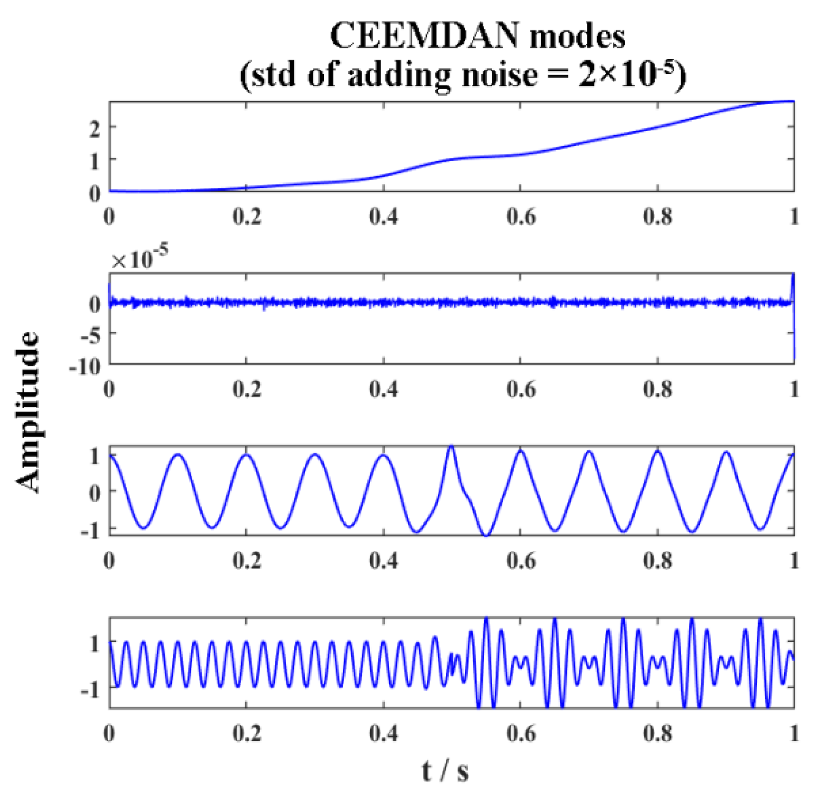
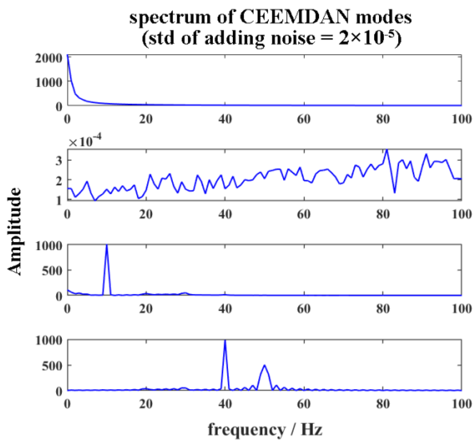
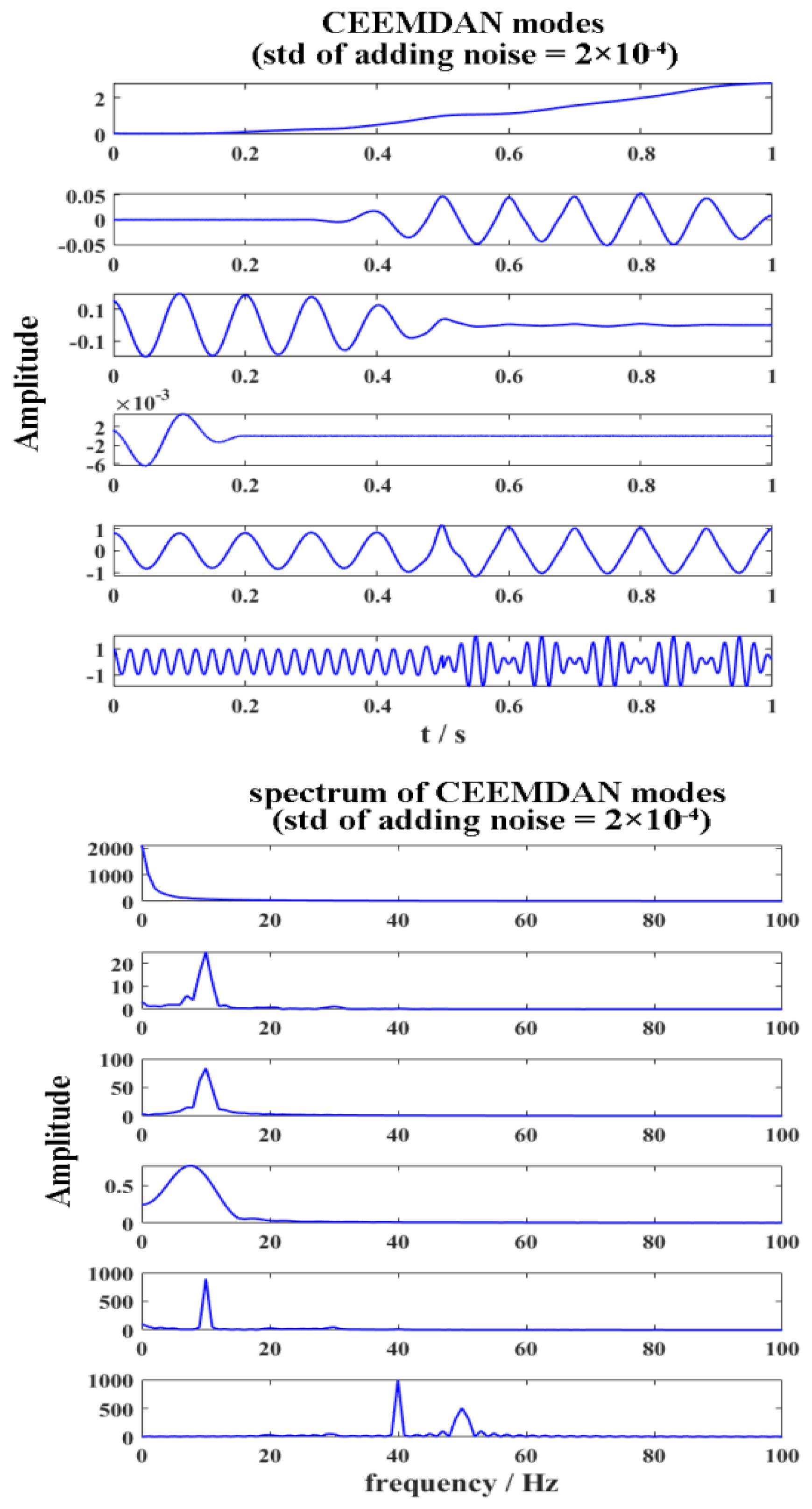
3.2. CEEMDAN
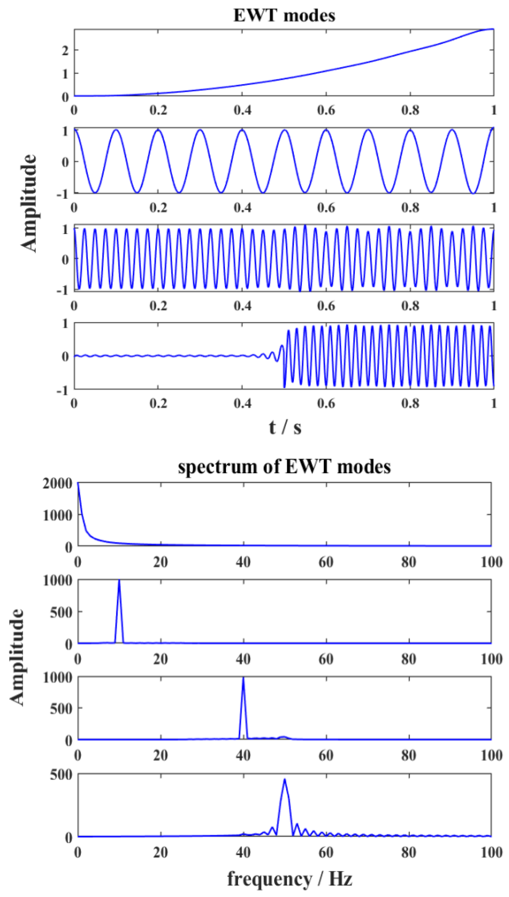
3.3. EWT
4. Results and Discussion
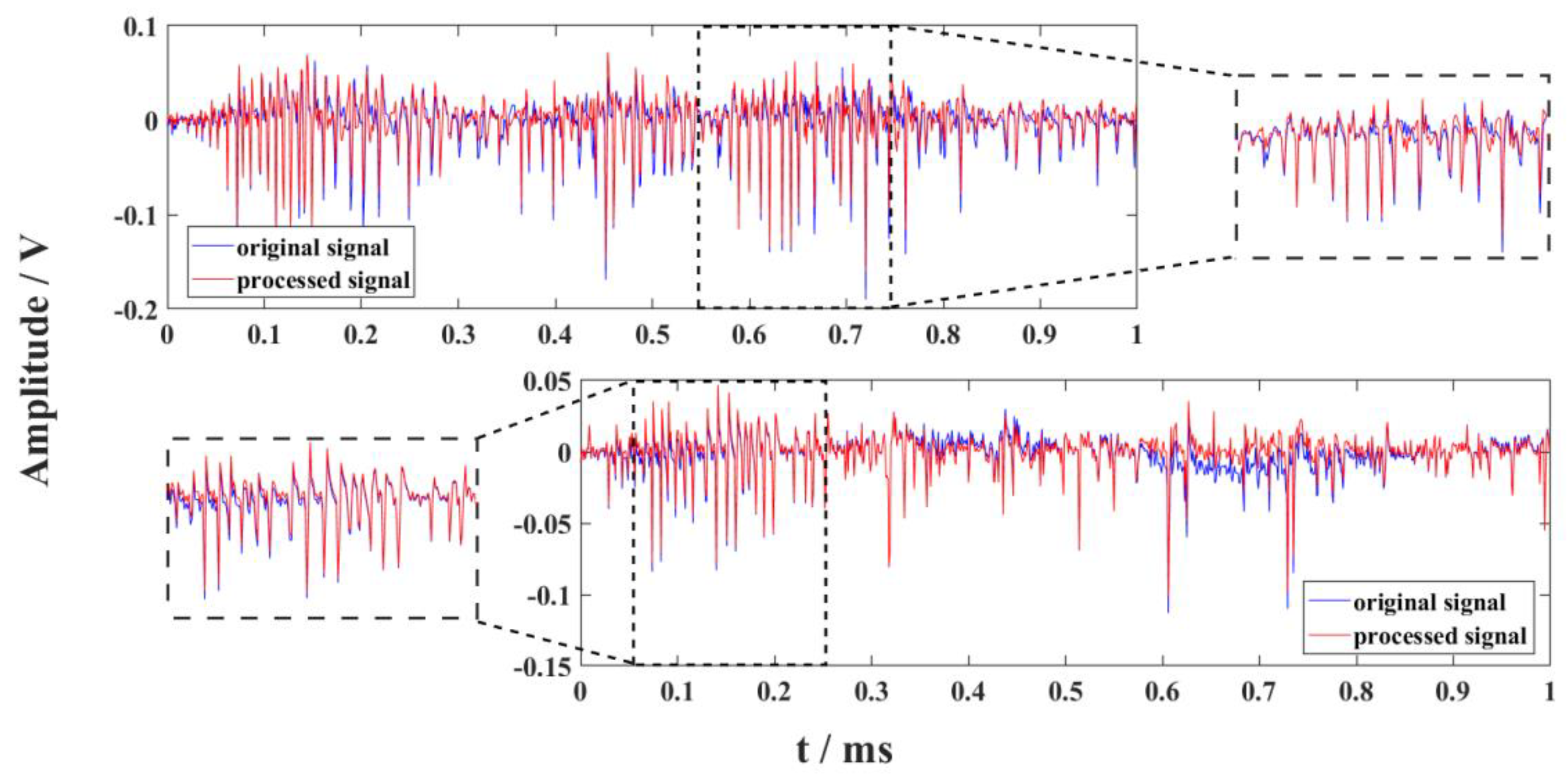
4.1. Results of Artificial Data
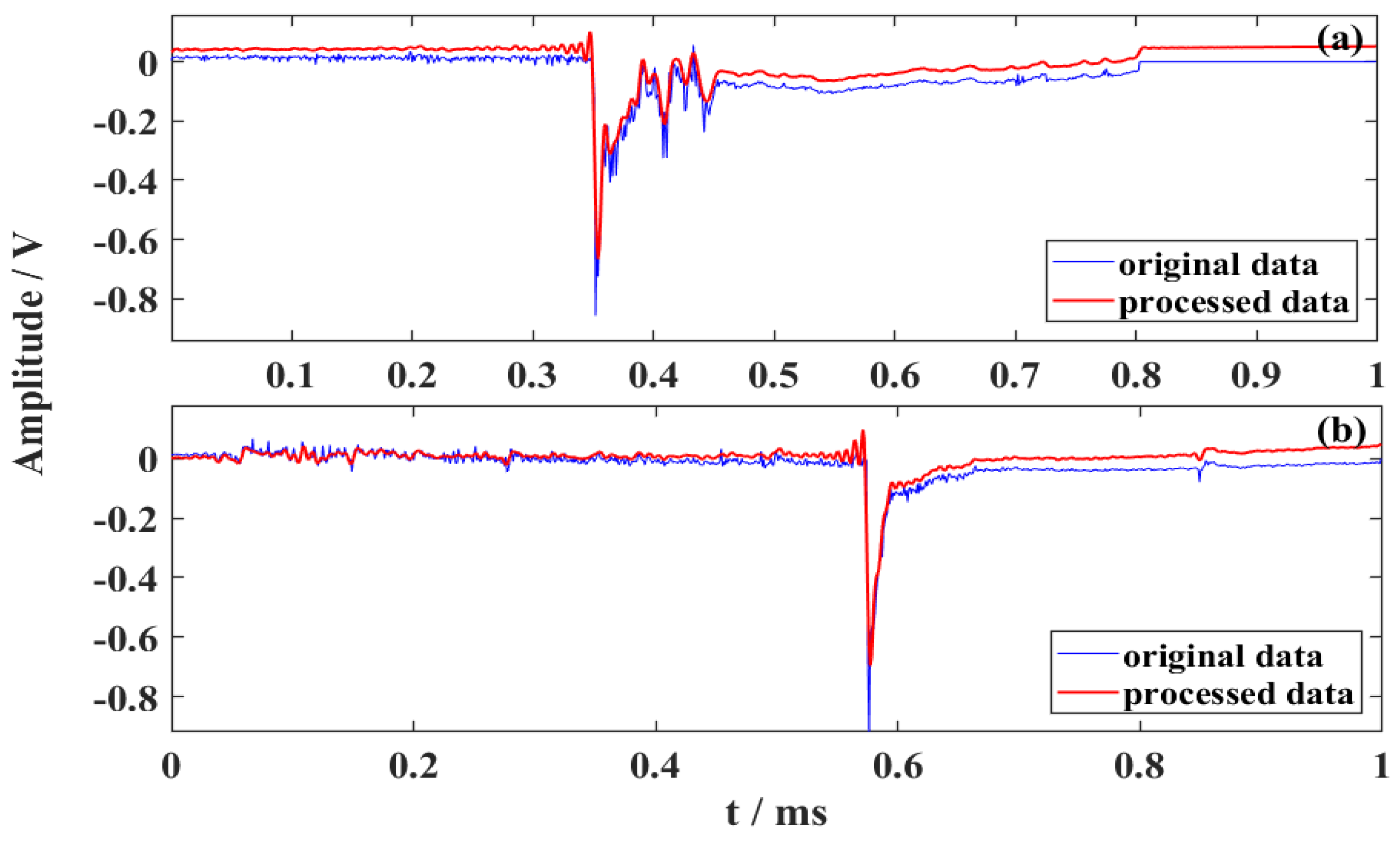
4.2. Results of FDTD Computing Lightning Signal with White Noise
4.3. Signals of Natural Lightning
4.3.1. MEWT Method
- The step-leaders’ modulus of each frequency distributes more evenly compared to CG lightning and cloud pulse.
- Although there are more high-frequency components in the received cloud flash signal than the ground flash, the main frequency band is below 150 kHz. This is not the case with step-leaders.
- Most of the energy of the ground flashback signal is concentrated below 50 kHz.
- After dividing the signal according to the above frequency bands, the kurtosis of noise and lightning signal is obviously different.
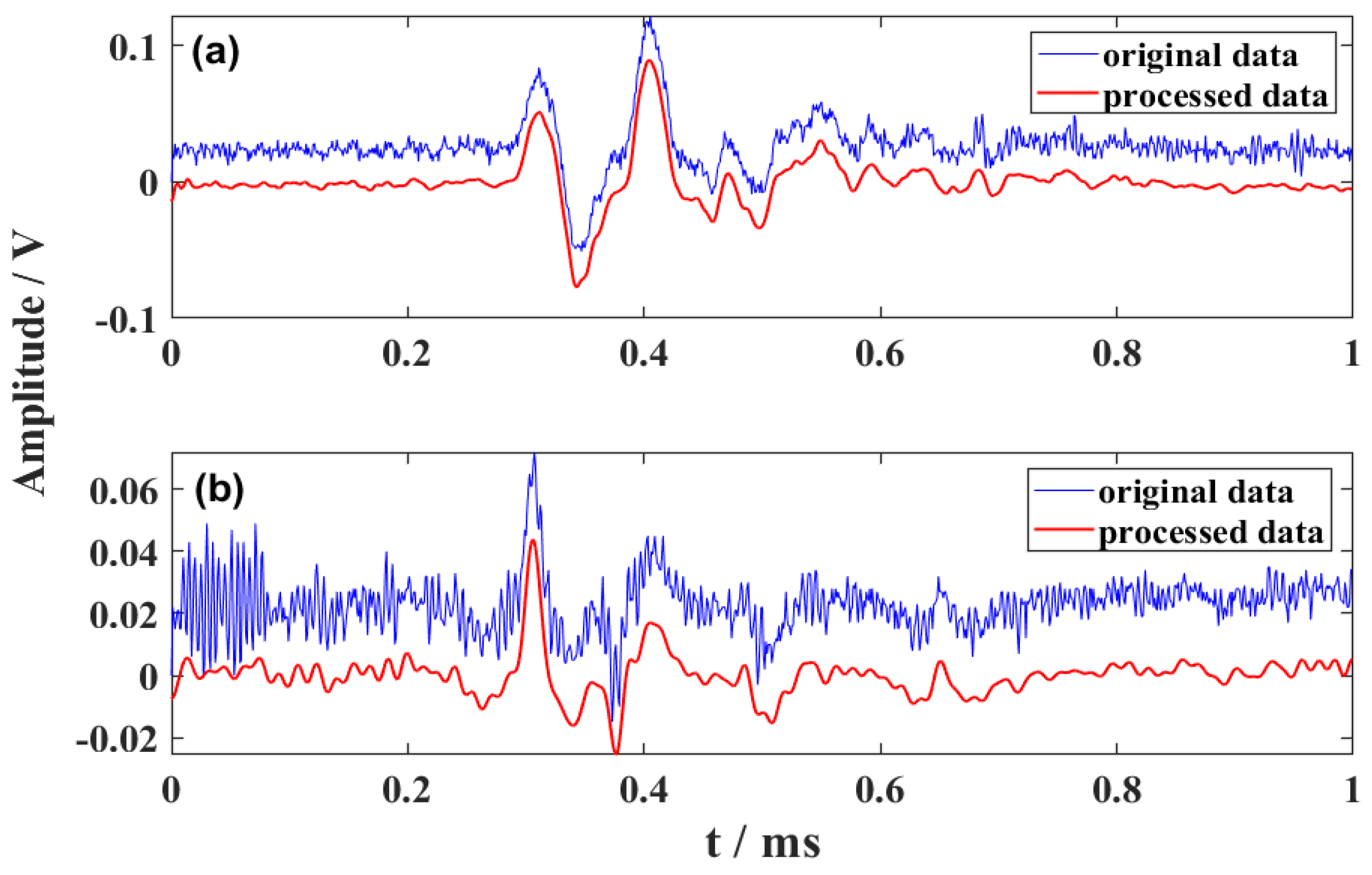
4.3.2. Processed Results of Different Classic Physical Processes of Lightning
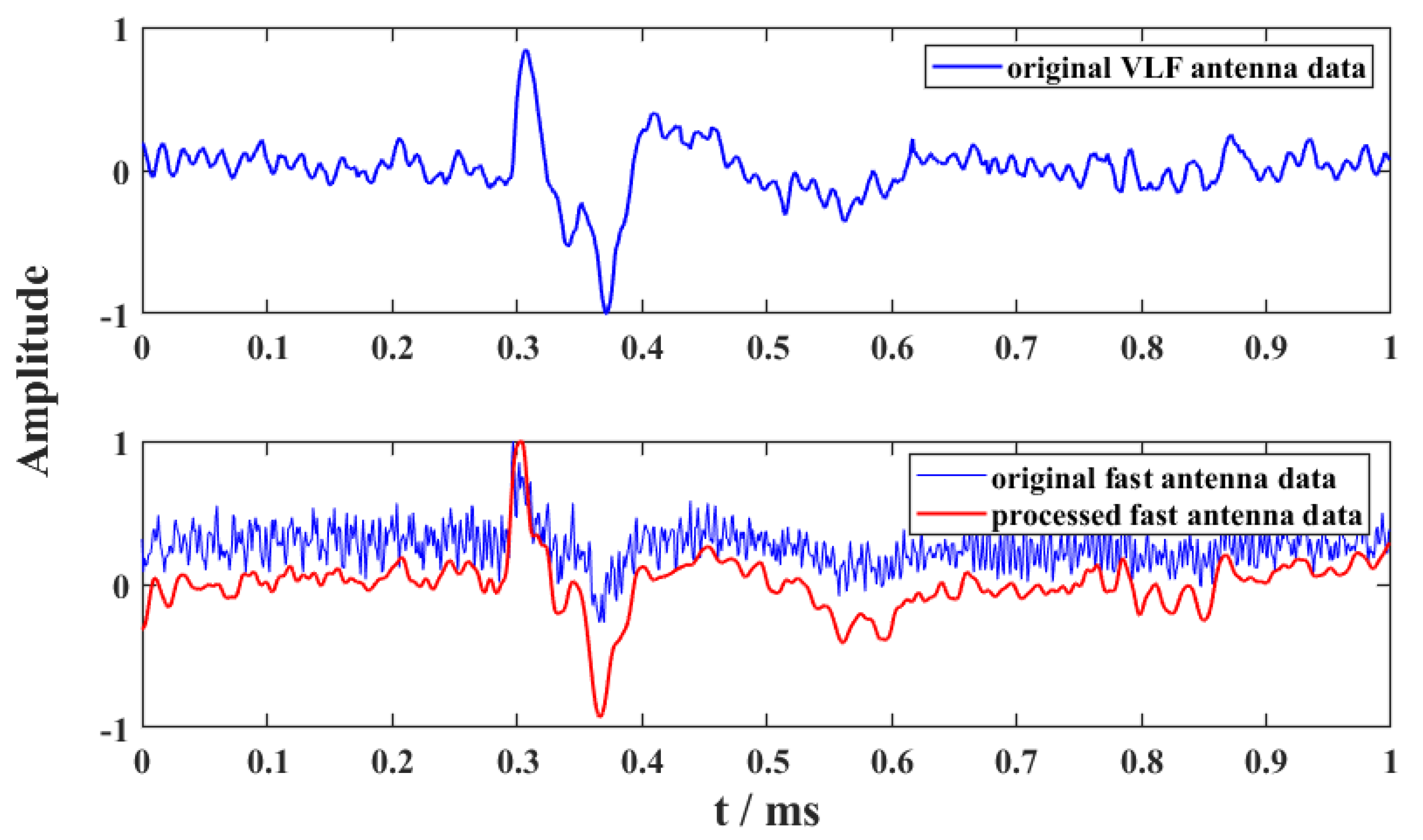
4.3.3. Processed Results of Lightning with Different Distance
5. Conclusions and Discussion
Author Contributions
Funding
Data Availability Statement
Conflicts of Interest
Abbreviations
| CD | Chengdu |
| CEEMDAN | Complete Ensemble Empirical Mode Decomposition With Adaptive Noise |
| CF | Chifeng |
| CWP | Chaiwopu |
| CG | Cloud-To-Ground |
| EMD | Empirical Mode Decomposition |
| EEMD | Ensemble Empirical Mode Decomposition |
| EWT | Empirical Wavelet Transform |
| FDTD | Finite Difference Time Domain |
| IMF | Intrinsic Mode Function |
| JQ | Jiuquan |
| LF/VLF | Low Frequency/Very Low Frequency |
| MEWT | Modified Empirical Wavelet Transform |
| NJ | Nanjing |
| NLLN | Nanjing Lightning Location Network |
| NWLLS NUIST | Wide-range Lightning Location System |
| SST | Synchrosqueezing Wavelet Transform |
| TY | Taiyuan |
| WF | Wavelet Transform |
| WH | Wuhan |
References
- Huanyi, L.; Wansheng, D. 3D spatial-temporal characteristics of initial breakdown process in lightning observed by broadband interferometer. J. Appl. Meteorol. Sci. 2016, 27, 16–24. [Google Scholar]
- Huang, N.E.; Shen, Z.; Long, S.R.; Wu, M.C.; Shih, H.H.; Zheng, Q.; Yen, N.-C.; Tung, C.C.; Liu, H.H. The empirical mode decomposition and the Hilbert spectrum for nonlinear and non-stationary time series analysis. Proc. R. Soc. London. Ser. A 1998, 454, 903–995. [Google Scholar] [CrossRef]
- Wu, Z.; Huang, N.E. Ensemble empirical mode decomposition: A noise-assisted data analysis method. Adv. Adapt. Data Anal. 2009, 1, 1–41. [Google Scholar] [CrossRef]
- Güzel, E.; Canyilmaz, M.; Türk, M. Application of wavelet-based denoising techniques to remote sensing very low frequency signals. Radio Sci. 2011, 46, 1–9. [Google Scholar] [CrossRef]
- Serhan, G.I.; Uman, M.A.; Childers, D.G.; Lin, Y.T. The RF spectra of first and subsequent lightning return strokes in the 1-to 200-km range. Radio Sci. 1980, 15, 1089–1094. [Google Scholar] [CrossRef]
- Rojas, H.E.; Cortés, C.A. Denoising of measured lightning electric field signals using adaptive filters in the fractional Fourier domain. Measurement 2014, 55, 616–626. [Google Scholar] [CrossRef]
- Peng, L.; Yi, Z.; Yijun, Z. Denoising methods of lightning transient electrical signals. High Power Laser Part Beams 2007, 19, 2055–2059. [Google Scholar]
- Huo, Y.L.; Zhang, G.S.; Lu, S.H.; Wang, Y.H.; Li, Y.J. Lightning signals denoising with double density dual tree wavelet transform. Laser Infrared 2013, 43, 1076–1079. [Google Scholar]
- Gao, T.C.; Han, X.D.; Qiu, S.; Ai, W.H.; Liu, X.C. Electric-field changes meter signal de-noising based on multi-wavelet transform. J. PLA Univ. Sci. Technol. (Nat. Sci. Ed.) 2009, 10, 90–94. [Google Scholar]
- Huo, Y.-L.; Yuan, P.-Y.; Qi, Y.-F. Denoising of Lightning Electric Field Signals Based on EMD-Wavelet Method. DEStech Trans. Eng. Technol. Res. 2016. [Google Scholar] [CrossRef][Green Version]
- Daubechies, I.; Lu, J.; Wu, H.T. Synchrosqueezed wavelet transforms: An empirical mode decomposition-like tool. Appl. Comput. Harmon. Anal. 2011, 30, 243–261. [Google Scholar] [CrossRef]
- Fan, X.P.; Zhang, Y.J.; Zheng, D.; Zhang, Y.; Lyu, W.T.; Liu, H.Y.; Xu, L.T. A new method of three-dimensional location for low-frequency electric field detection array. J. Geophys. Res. Atmos. 2018, 123, 8792–8812. [Google Scholar] [CrossRef]
- Fan, X.; Zhang, Y.; Krehbiel, P.R.; Zhang, Y.; Zheng, D.; Yao, W.; Xu, L.; Liu, H.; Lyu, W. Application of ensemble empirical mode decomposition in low-frequency lightning electric field signal analysis and lightning location. IEEE Trans. Geosci. Remote Sens. 2020, 59, 86–100. [Google Scholar] [CrossRef]
- Torres, M.E.; Colominas, M.A.; Schlotthauer, G.; Flandrin, P. A complete ensemble empirical mode decomposition with adaptive noise. In Proceedings of the 2011 IEEE International Conference on Acoustics, Speech and Signal Processing (ICASSP), Prague, Czech Republic, 22–27 May 2011; pp. 4144–4147. [Google Scholar]
- Colominas, M.A.; Schlotthauer, G.; Torres, M.E.; Flandrin, P. Noise-assisted EMD methods in action. Adv. Adapt. Data Anal. 2014, 4, 1250025. [Google Scholar] [CrossRef]
- Gilles, J. Empirical wavelet transform. IEEE Trans. Signal Process. 2013, 61, 3999–4010. [Google Scholar] [CrossRef]
- Feng, Z.; Zhang, D.; Zuo, M.J. Adaptive mode decomposition methods and their applications in signal analysis for machinery fault diagnosis: A review with examples. IEEE Access 2017, 5, 24301–24331. [Google Scholar] [CrossRef]
- Huang, S.; Kong, W.; Yang, J.; Zhang, Q.; Yao, N.; Dai, B.; Gu, J. Distinguishing different lightning events based on wavelet packet transform of magnetic field signals. J. Atmos. Sol. Terr. Phys. 2020, 211, 105477. [Google Scholar] [CrossRef]
- Gilles, J.; Heal, K. A parameterless scale-space approach to find meaningful modes in histograms—Application to image and spectrum segmentation. Int. J. Wavelets Multiresolution Inf. Process. 2014, 12, 1450044. [Google Scholar] [CrossRef]
- Otsu, N. A threshold selection method from gray-level histograms. IEEE Trans. Syst. Man Cybern. 1979, 9, 62–66. [Google Scholar] [CrossRef]
- Hou, W.; Zhang, Q.; Zhang, J.; Wang, L.; Shen, Y. A new approximate method for lightning-radiated ELF/VLF ground wave propagation over intermediate ranges. Int. J. Antennas Propag. 2018, 2018. [Google Scholar] [CrossRef]
- Dwyer, J.R.; Uman, M.A. The physics of lightning. Phys. Rep. 2017, 534, 147–241. [Google Scholar] [CrossRef]


Publisher’s Note: MDPI stays neutral with regard to jurisdictional claims in published maps and institutional affiliations. |
© 2022 by the authors. Licensee MDPI, Basel, Switzerland. This article is an open access article distributed under the terms and conditions of the Creative Commons Attribution (CC BY) license (https://creativecommons.org/licenses/by/4.0/).
Share and Cite
Dai, B.; Li, J.; Zhou, J.; Zeng, Y.; Hou, W.; Zhang, J.; Wang, Y.; Zhang, Q. Application of a Modified Empirical Wavelet Transform Method in VLF/LF Lightning Electric Field Signals. Remote Sens. 2022, 14, 1308. https://doi.org/10.3390/rs14061308
Dai B, Li J, Zhou J, Zeng Y, Hou W, Zhang J, Wang Y, Zhang Q. Application of a Modified Empirical Wavelet Transform Method in VLF/LF Lightning Electric Field Signals. Remote Sensing. 2022; 14(6):1308. https://doi.org/10.3390/rs14061308
Chicago/Turabian StyleDai, Bingzhe, Jie Li, Jiahao Zhou, Yingting Zeng, Wenhao Hou, Junchao Zhang, Yao Wang, and Qilin Zhang. 2022. "Application of a Modified Empirical Wavelet Transform Method in VLF/LF Lightning Electric Field Signals" Remote Sensing 14, no. 6: 1308. https://doi.org/10.3390/rs14061308
APA StyleDai, B., Li, J., Zhou, J., Zeng, Y., Hou, W., Zhang, J., Wang, Y., & Zhang, Q. (2022). Application of a Modified Empirical Wavelet Transform Method in VLF/LF Lightning Electric Field Signals. Remote Sensing, 14(6), 1308. https://doi.org/10.3390/rs14061308