Data-Driven Artificial Intelligence Model of Meteorological Elements Influence on Vegetation Coverage in North China

Abstract

Based on remote sensing data of vegetation coverage, observation data of basic meteorological elements, and support vector machine (SVM) method, this study develops an analysis model of meteorological elements influence on vegetation coverage (MEVC). The variations for the vegetation coverage changes are identified utilizing five meteorological elements (temperature, precipitation, relative humidity, sunshine hour, and ground temperature) in the SVM model. The performance of the SVM model is also evaluated on simulating vegetation coverage anomaly change by comparing with statistical model multiple linear regression (MLR) and partial least squares (PLS)-based models. The symbol agreement rates (SAR) of simulations produced by MLR, PLS, and SVM models are 55%, 57%, and 66%, respectively. The SVM model shows obviously better performance than PLS and MLR models in simulating meteorological elements-related interannual variation of vegetation coverage in North China. Therefore, the introduction of the intelligent analysis method in term of SVM in model development has certain advantages in studying the internal impact of meteorological elements on regional vegetation coverage. It can also be further applied to predict the future vegetation anomaly change.

1. Introduction

Vegetation is the key element for the interaction between land and atmosphere, and its change is caused by topographic (altitude, slope, and others) factors [1], human activities (urban construction, overgrazing, and ecological engineering), and climate change [2,3,4,5]. Among them, climate is one of the main determinants of vegetation type distribution and dynamic change [6,7].

Remote sensing data, such as vegetation coverage (VC), normalized difference vegetation index (NDVI), and net primary productivity (NPP), is widely applied in vegetation greenness, agriculture, forestry, hydrology, and drought detection [8,9,10,11]. Numerous studies explored the response of regional and global vegetation to climate change. Zhao et al. [12] revealed that growing-season NDVI depends largely on water in arid and semiarid areas, temperature in high northern latitude areas, and radiation in the Amazon and Eastern and Southern Asia. Li et al. [13] used linear correlation and showed that there was a strong correlation between grassland and precipitation, forest, farmland, and temperature in the North China Plain. Previous studies usually use linear correlation and partial correlation analysis to study the relationship between the vegetation coverage and meteorological elements in the same or advanced period, to explain that the main driving factors of vegetation dynamic changes in different climatic regions and seasons [2,12,13,14,15,16]. Scholars mainly also analyze the key driving factors affecting vegetation growth. However, how to use an effective method to quantify the influence of meteorological elements on the vegetation coverage and establish the proper model remains a difficult problem in ecological meteorology research.

Vegetation models, such as global dynamic vegetation model (DGVM), statistical models, and machine learning, are an effective tool to quantitatively understand the interaction between climate and vegetation. DGVM, such as LPJ-DGVM (the Lund–Potsdam–Jena Dynamic Global Vegetation Model) simulated vegetation changes in high-latitude areas of the Northern Hemisphere [17]. Although the simulation effect of the global dynamic vegetation model is excellent, its limitation is that it is not easy to obtain a large number of model input data, parameter data, and validation data [18]. On the contrary, statistical models and machine learning can overcome the data problem, so they are commonly used in the simulation of vegetation dynamic change, especially in local or small institutions with limited infrastructure capability. A number of studies have focused on climate prediction of vegetation change [12,13,19,20]. Based on vegetation coverage and meteorological elements data, such as temperature, precipitation, and sunshine hours in North China during 2000 to 2018, Bai proposed a statistical model that suggests that meteorological elements affect vegetation coverage [21]. Machine learning has been extensively used in ecology, meteorology, and other fields, and performs well. Zheng et al. [22] used stepwise cluster algorithm combined with GIMMS (Global Inventory Modelling and Mapping Studies) AVHRR (Advanced Very High Resolution Radiometer) NDVI datasets (2000–2013) to study the relationship between temperature, precipitation, and NDVI in the Three-River Headwaters region of China, and proved the significant influence of precipitation and temperature on NDVI. Shi et al. [23] used an SVM-based classification method combined with Landsat images to determine vegetation area and vegetation distribution. Something these methods have in common is that computers intelligently dig out hidden laws through a large number of historical data and use them for prediction or classification [24].

Artificial intelligence (AI) is a method to explore the relationship between independent and dependent variables of a system according to the existing data, so that the model can make the most accurate estimation possible when the output is unknown [24,25]. Several algorithms, such as random forest regression, regression trees, and support vector regression, are applied to prediction of vegetation change [22,23,26]. SVM is a typical binary classification method which has the advantages of solving high-dimensional problems, dealing with nonlinear problems, and low generalization error rate. Based on the advantages of the SVM method, it is necessary to use SVM to build an analytical model to study the complex nonlinear relationship between meteorological elements and vegetation coverage.

North China is the main wheat-producing base in northern China, and the vegetation in this area is extremely sensitive to climate change. Studying the influence of meteorological elements (temperature (T), precipitation (P), relative humidity (R), sunshine hours (S), and ground temperature (G)) on the vegetation coverage in this area has crucial value for improving the agricultural production. This paper aims to set up an AI model of meteorological elements’ influence on vegetation coverage (MEVC) in North China. The main framework of the article is as follows (Figure 1): Section 2 describes the location of the study area, data source, length and preprocessing, statistical method, and MEVC model; Section 3 analyzes the temporal and spatial characteristics of vegetation coverage and meteorological elements and introduces the influence factors of meteorological elements on vegetation coverage and MEVC model training, testing, and simulation. The discussion of research results and future work is given in Section 4. A conclusion is given in Section 5.

2. Materials and Methods

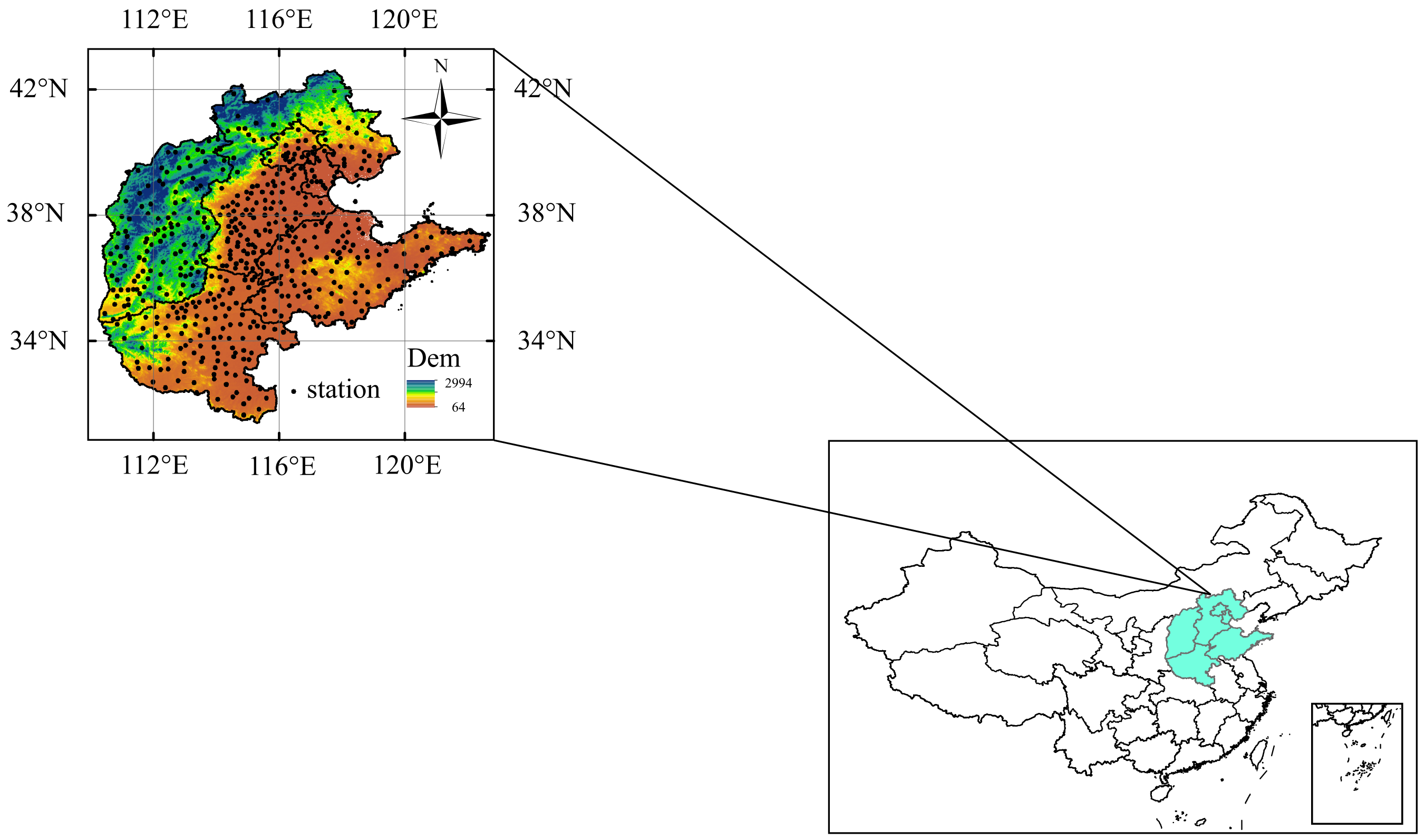
2.1. Study Area

Based on the main wheat-producing areas, this paper expands the North China region to Beijing, Tianjin, Shanxi, Shandong, Hebei, and Henan Province. For the convenience of description, it is still referred to as North China (Figure 2). The scope of the study area is 31${}^{\circ }$–42${}^{\circ }$ N and 110${}^{\circ }$–122${}^{\circ }$ E, covering an area of about 696,600 square kilometers. The altitude in the northwest is high and the altitude in the southeast is low. According to the distribution of total precipitation in summer (Figure 3b1), North China is in the transition zone of semiarid and semihumid (0–200 mm is arid zone, 200–400 mm is semiarid zone, and 400–600 mm is semihumid zone), of which the northwest is semiarid zone and the southeast is semihumid zone [27]. Studies have shown that North China has been changing to warm and dry since 1950, so the vegetation in this area is extremely sensitive to climate change [28]. Therefore, it is quite necessary to study the influence of meteorological elements on vegetation coverage in this area.

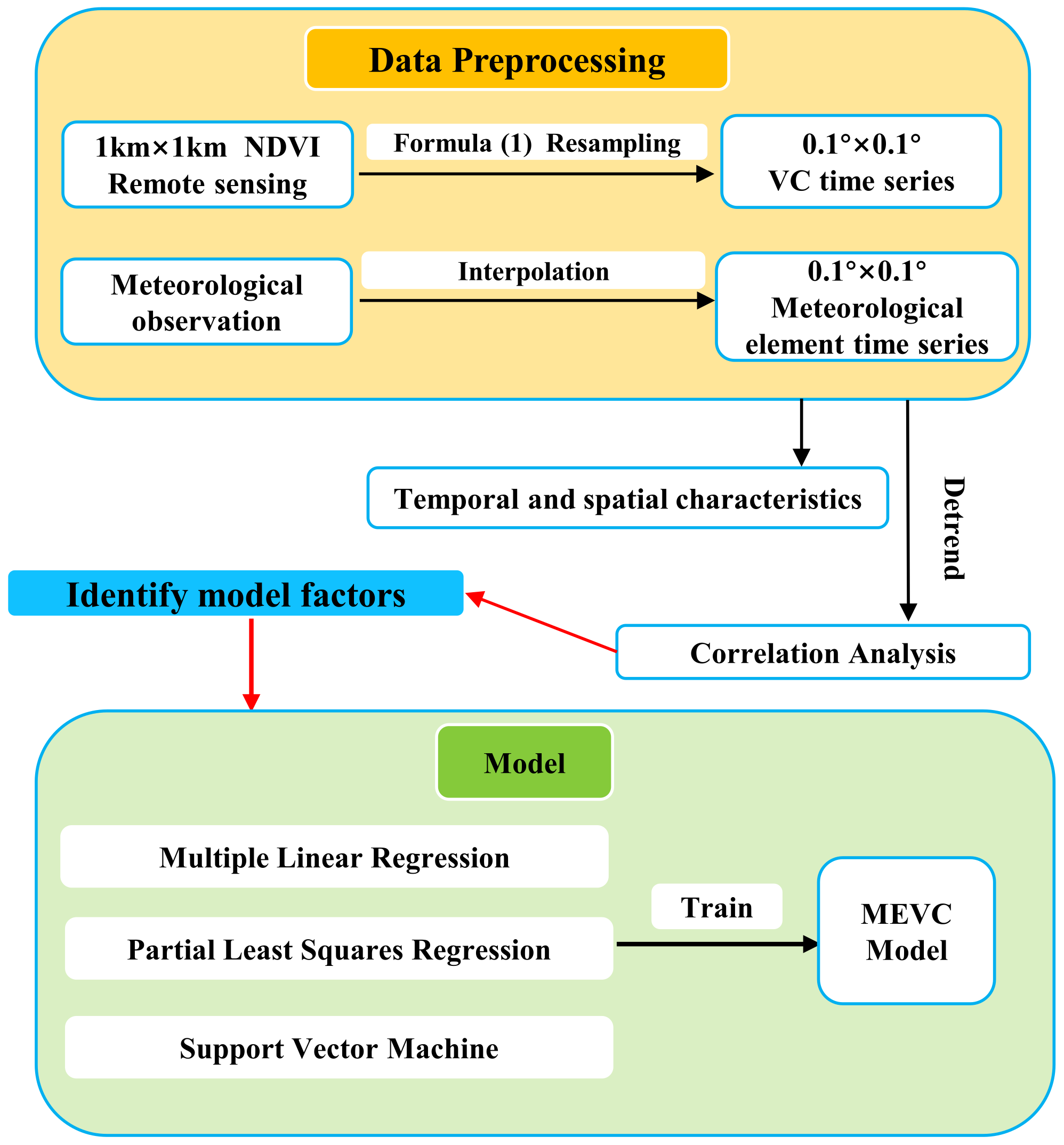
2.2. Data and Preprocessing

Vegetation coverage data: The $NDVI$ data in Moderate-resolution Imaging Spectroradiometer (MODIS) 1 km monthly synthetic products (https://earthdata.nasa.gov/, accessed on 24 October 2021) are used to calculate the vegetation according to Formula (1) [8]:

$$VC=\frac{NDVI-NDV{I}_S}{NDV{I}_V-NDV{I}_S}.$$

(1)

where $NDV{I}_S$ represents the $NDVI$ value of pixels without vegetation cover during 2000 to 2018, and $NDV{I}_V$ represents the $NDVI$ value of pixels completely covered by vegetation. Considering that this paper studies a single pixel with spatial distribution, the high resolution of 0.01${}^{\circ }$× 0.01${}^{\circ }$ makes the amount of calculation very large. In order to improve the calculation efficiency, the data resolution is appropriately reduced to 0.1${}^{\circ }$× 0.1${}^{\circ }$.

Meteorological data: daily 2 m atmospheric temperature (T), precipitation (P), relative humidity (R), sunshine hours (S), and 0 cm ground temperature (G) data in North China are selected from the 2400 stations dataset provided by the National Meteorological Information Center. All the stations with missing data are removed, and the remaining are used for North China research, a total of 525 stations. The specific locations of North China stations are shown in Figure 2. For detailed stations information, please visit http://data.cma.cn, accessed on 25 February 2022. The data length is from 2000 to 2018. We calculated the monthly average of $T,R,S,G$, and total monthly P for each station, and obtained the grid data with 0.1${}^{\circ }$ × 0.1${}^{\circ }$ resolution by using the inverse distance weighted interpolation method to be consistent with the resolution of vegetation coverage data.

2.3. Methodology

The trend approach was applied in the analysis vegetation coverage ($VC$) and meteorological elements $(T,P,R,S,G)$ variation trends:

$$slop{e}^{ij}=\frac{n\times {\displaystyle \sum _{t=1}^n}t\times x_t^{ij}-{\displaystyle \sum _{t=1}^n}t{\displaystyle \sum _{t=1}^n}{x}_t^{ij}}{n\times {\displaystyle \sum _{t=1}^n}{t}^2-{({\displaystyle \sum _{t=1}^n}t)}^2},$$

(2)

where $slop{e}^{ij}$ is variation trend of row i and column j; n is the years of study; and $x_t^{ij}$ is variable $x(T,P,R,S,G,VC)$ of row i and column j of year t.

Correlation analysis is a statistical method to explore the relationship between two variables. Here, the significance is tested by Student’s t test. The correlation coefficient formula is

$$r_{xy}^{ij}=\frac{{\displaystyle \sum _{t=1}^n}(x_t^{ij}-{\overline{x}}^{ij})(y_t^{ij}-{\overline{y}}^{ij})}{\sqrt{{\displaystyle \sum _{t=1}^n}{(x_t^{ij}-{\overline{x}}^{ij})}^2{\displaystyle \sum _{t=1}^n}{(y_t^{ij}-{\overline{y}}^{ij})}^2}},$$

(3)

where $r_{xy}^{ij}$ is correlation coefficient of the variable $x^{ij}$ and variable $y^{ij}$; $x_t^{ij}$ is x of row i and column j of year t; $y_t^{ij}$ is y of row i and column j of year t; ${\overline{x}}^{ij}$ is the mean for any $x^{ij}$; ${\overline{y}}^{ij}$ is the mean for any $y^{ij}$.

We use the $SAR$ to evaluate model performance; the $SAR$ is calculated as

$$SAR=\frac{N_g}{N}.$$

(4)

where N represents the total number of pixels and $N_g$ represents the number of pixels with the same symbols of observed and simulated vegetation cover changes of pixels.

2.4. Influence Model of Meteorological Elements on the Vegetation Coverage

In order to describe the MEVC, based on the meteorological elements and vegetation coverage data during 2000–2018, the MEVC model is constructed by using SVM [29,30], PLS [31,32], and MLR [33] methods, respectively.

(1)

The MEVC model based on SVM

The influence of meteorological elements on vegetation coverage has a complex nonlinear relationship, but solving nonlinear problems is not easy, so we transform the nonlinear problem into a linear problem by performing a nonlinear transformation. The classification hyperplane equation of the influence of the meteorological element on the symbol change of vegetation coverage can be given:

$${\omega }^T\phi (T,P,R,S,G)+b=0.$$

(5)

In Equation (5), $\omega$ is the weight vector, $\phi$ is a nonlinear transformation, and b is a constant. According to the principle of structural risk minimization, the corresponding classification decision function is

$$f(T,P,R,S,G)=sign({\omega }^T\phi (T,P,R,S,G)+b).$$

(6)

which side of the hyperplane the sample is located on is determined by the sign of $f(T,P,R,S,G)$. The plane with the maximum distance between the hyperplane and the sample set of both vegetation increase and vegetation decrease is the optimal classification hyperplane [34]. Suppose the nearest point is $(T_i,P_i,R_i,S_i,G_i)$, the hyperplane satisfies $|\omega ·\phi (T_i,P_i,R_i,S_i,G_i)+b|=1$, but some samples cannot be classified correctly through Equation (6). Then, we introduce relaxation variables to correctly classify the wrong points. Moreover, we need to give them a penalty, represented by C in Equation (7). Solving Equations (5) and (6) transform into solving the constrained optimization problem, that is

$$\left\{\begin{array}{cc}\hfill & \underset{\omega ,b}{min}\frac{1}{2}{\left|\right|\omega \left|\right|}^2+C\sum _{i=1}^t{\mu }_i,\hfill \\ \hfill & s.t.sign\left(VC{R}_i\right)[\omega ·\phi (T_i,P_i,R_i,S_i,G_i)+b]-1+{\mu }_i\ge 0,i=1,2,\cdots ,t,\hfill \\ \hfill & {\mu }_i\ge 0.\hfill \end{array}\right.$$

(7)

We use the Lagrange multiplier method to solve the constrained optimization problem, where the Lagrange function is constructed as

$$\begin{array}{cc}\hfill L(\omega ,b,\mu ,\tau ,\rho )=& \frac{1}{2}{\left|\right|\omega \left|\right|}^2+C\sum _{i=1}^t{\mu }_i-\sum _{i=1}^t{\tau }_i\left(sign\left(VC{R}_i\right)\right)(\omega ·\phi (T_i,P_i,R_i,S_i,G_i)+b]-1+{\mu }_i)\hfill \\ \hfill & -\sum _{i=1}^t{\rho }_i{\mu }_i,\hfill \end{array}$$

(8)

where (${\tau }_i,{\rho }_i$ ) is Lagrange multiplier. The constrained optimization problem of (7) is equivalent to solving $\underset{\omega ,b,\mu }{min}\underset{\tau ,\rho }{max}L(\omega ,b,\mu ,\tau ,\rho )$. When the Karush–Kuhn–Tucker (KKT) condition is satisfied, $\underset{\omega ,b,\mu }{min}\underset{\tau ,\rho }{max}L(\omega ,b,\mu ,\tau ,\rho )$ is equivalent to $\underset{\tau ,\rho }{max}\underset{\omega ,b,\mu }{min}L(\omega ,b,\mu ,\tau ,\rho )$. The partial derivatives of $L(\omega ,b,\mu ,\tau ,\rho )$ with respect to $\omega ,b$ and ${\mu }_i$, are

$$\begin{array}{cc}\hfill & \frac{\partial L}{\partial \omega }=\omega -\sum _{i=1}^t{\tau }_{i}sign\left(VC{R}_i\right)\phi (T_i,P_i,R_i,S_i,G_i),\hfill \\ \hfill & \frac{\partial L}{\partial b}=-\sum _{i=1}^t{\tau }_{i}sign\left(VC{R}_i\right)\hfill \\ \hfill & \frac{\partial L}{\partial {\mu }_i}=C-{\tau }_i-{\rho }_i\hfill \end{array}$$

(9)

Let Equation (9) be equal to 0, then one can obtain

$$\begin{array}{cc}\hfill & \omega =\sum _{i=1}^t{\tau }_{i}sign\left(VC{R}_i\right)\phi (T_i,P_i,R_i,S_i,G_i),\hfill \\ \hfill & \sum _{i=1}^t{\tau }_{i}sign\left(VC{R}_i\right)=0,\hfill \\ \hfill & C={\tau }_i-{\rho }_i.\hfill \end{array}$$

(10)

Substituting Equations (10) into Equation (8), we can deduce

$$\left\{\begin{array}{cc}\hfill & \underset{\tau }{max}\frac{1}{2}\sum _{i=1}^t\sum _{j=1}^{t}sign\left(VC{R}_i\right)sign\left(VC{R}_j\right)\phi (T_i,P_i,R_i,S_i,G_i)\phi (T_j,P_j,R_j,S_j,G_j),\hfill \\ \hfill & s.t.\sum _{i=1}^t{\tau }_{i}sign\left(VC{R}_i\right)=0,0\le {\tau }_i\le C.\hfill \end{array}\right.$$

(11)

In Equation (12), we find the optimal solution ${\tau }^{*}={({\tau }_1^{*},{\tau }_2^{*},\cdots ,{\tau }_t^{*})}^T$ by using the sequential minimal optimization (SMO) method, then the calculation

$b^{*}=sign\left(VC{R}_j\right)-{\displaystyle \sum _{i=1}^t}{\tau }_i^{*}sign\left(VC{R}_i\right)\phi (T_i,P_i,R_i,S_i,G_i)·\phi (T_j,P_j,R_j,S_j,G_j).$

Thus, the classification hyperplane is

$f(T,P,R,S,T)=sign({\displaystyle \sum _{i=1}^t}{\tau }_i^{*}sign\left(VC{R}_i\right)\phi (T_i,P_i,R_i,S_i,G_i)·\phi (T,P,R,S,G)+b^{*}),$ where

$$\begin{array}{cc}\hfill \phi (T_i,P_i,R_i,S_i,G_i)·\phi (T,P,R,S,G)=& exp(-\gamma ({(T-T_i)}^2+{(P-P_i)}^2+{(R-R_i)}^2\hfill \\ & +{(S-S_i)}^2+{(G-G_i)}^2\left)\right),\hfill \end{array}$$

Through the above derivation process, the MEVC model based on SVM is given:

$$\begin{array}{cc}\hfill f(T,P,R,S,T)=& sign(\sum _{i=1}^t{\tau }_i^{*}sign\left(VC{R}_i\right)exp(-\gamma ({(T-T_i)}^2+{(P-P_i)}^2+{(R-R_i)}^2\hfill \\ \hfill & +{(S-S_i)}^2+{(G-G_i)}^2\left)\right)+b^{*}),{\tau }_i^{*}\in [0,C].\hfill \end{array}$$

(12)

(2)

The MEVC model based on PLS and MLR

In order to quantify the influence of meteorological elements on vegetation coverage, Bai [21] constructed a linear model, Equation (13):

$$VCR=a_0+a_{1}T+a_{2}P+a_{3}R+a_{4}S+a_{5}G+\epsilon .$$

(13)

where $a_0,a_1,a_2,a_3,a_4,a_5$ are the fitting parameters and $\epsilon$ is the error term. The parameters are trained by MLR and PLS methods, and two linear models (MLR model, PLS model) are obtained, respectively.

2.5. Identify Model Factors and Parameter Sensitivity Analysis

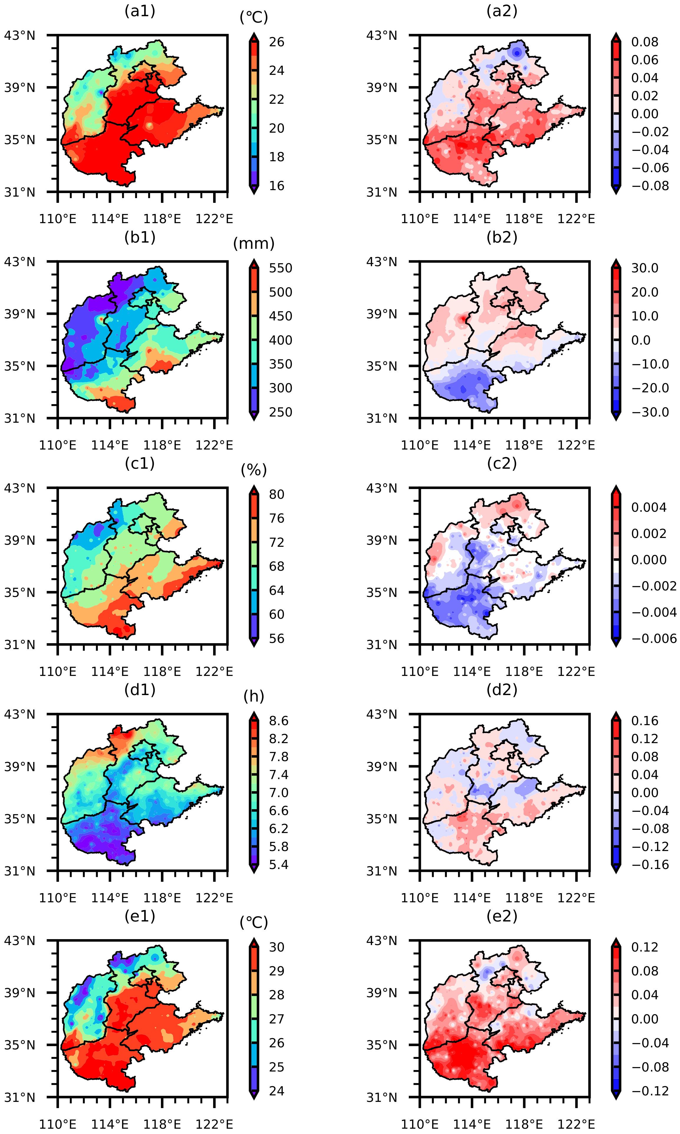
2.5.1. Temporal and Spatial Characteristics of Meteorological Elements and Vegetation Coverage

The temperature, precipitation, relative humidity, and ground temperature gradually increase from northwest to southeast, and the sunshine hours gradually decrease from northwest to southeast in North China (Figure 3a1–e1). Therefore, the climate in this region mainly presents the distribution characteristics of northwest–southeast-type. The summer temperature and precipitation in most areas of North China show an upward trend and the relative humidity shows a downward trend, indicating that North China is continuously changing to warm and dry (Figure 3a2–e2). Except for the low vegetation coverage in the northwest of North China, the vegetation coverage in other areas basically reaches more than 0.6 (Figure 4a). The vegetation coverage shows an increasing trend (Figure 4b), which is mainly related to the state ecological restoration projects implemented in terms of afforestation, returning farmland to forest, Three-North Shelterbelt, etc. [9,35,36,37]. Therefore, when we carry out the work of the influence of meteorological elements on vegetation coverage, we roughly regard the linear trend of vegetation coverage as the impact of human factors and the fluctuation as the variation caused by the fluctuation of meteorological elements [14,16]. The vegetation coverage analyzed in the following study is also treated with linear trend removed. By analyzing the temporal and spatial characteristics of summer meteorological elements and vegetation coverage in North China, it is obvious that the vegetation coverage in Northwest China is low, while the air temperature, ground temperature, precipitation, and relative humidity are low, and sunshine hours are long, which implies that these elements have a great influence on vegetation coverage change in North China.

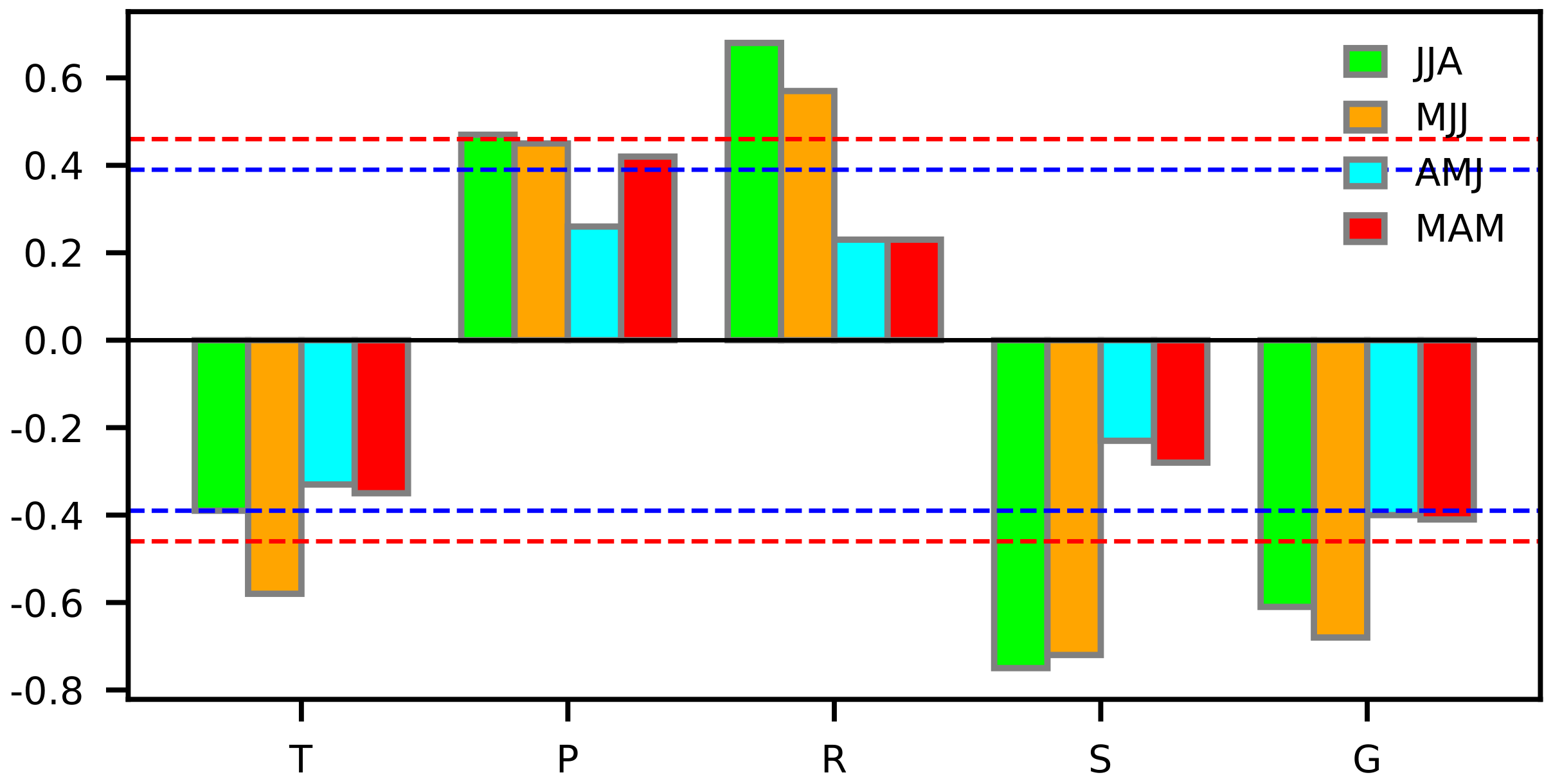
2.5.2. Relationship between Vegetation Coverage and Meteorological Elements

According to the physiological process of vegetation growth, meteorological elements (such as temperature, precipitation, relative humidity, sunshine hours, and ground temperature) have a certain continuous (cumulative) and lag effect on the growth of vegetation [38,39,40]. The selection of key factors is based on the correlation analysis between summer vegetation coverage and each meteorological element with the same period (summer, JJA), one month ahead (MJJ), two months ahead (AMJ), and one season ahead (MAM). Correlation analysis between vegetation coverage and meteorological element shows that vegetation coverage was positively correlated with precipitation and relative humidity, but it shows negative correlation with air temperature, sunshine hours, and ground temperature. Influence of meteorological elements of AMJ and MAM on vegetation coverage are not significant (Figure 5). Observing Figure 5, it is obvious that the main meteorological factors affecting vegetation growth are precipitation, relative humidity, sunshine hours of JJA, and air temperature and ground temperature of MJJ.

Temperature is significantly correlated with sunshine hours and ground temperature; precipitation is significantly correlated with relative humidity; relative humidity is significantly correlated with precipitation, sunshine hours, and ground temperature; sunshine hours are significantly correlated with temperature, relative humidity, and ground temperature; ground temperature is significantly correlated with temperature, relative humidity, and sunshine hours (Figure 6). Therefore, it can be found that these five meteorological elements have interactions with each other, jointly influencing the physical process of vegetation growth in North China.

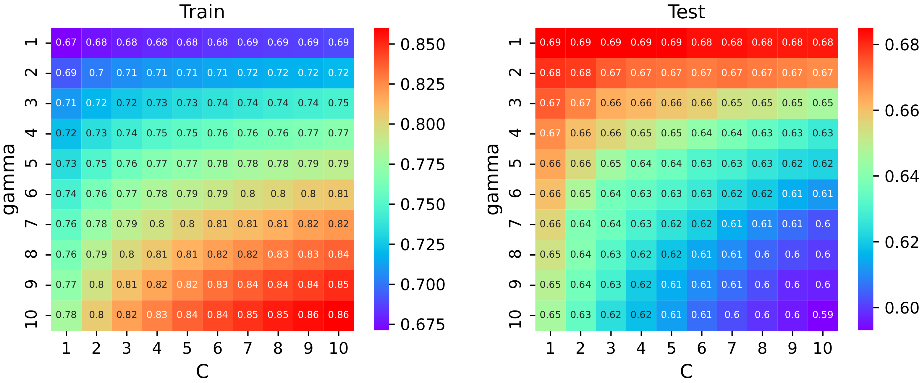
2.5.3. MEVC Model Training and Testing

We selected the above interpolation data of temperature (T) and ground temperature (G) from May to July, and precipitation (P), relative humidity (R), and sunshine hours (S) from June to August during 2000–2018. The three MEVC models were trained and tested by utilizing the fluctuation data of meteorological elements and vegetation coverage. Meteorological elements are defined as input, and the category of whether vegetation increases or decreases is regarded as the output of each model.

The training data of MEVC model is $(T_i,P_i,R_i,S_i,G_i,sign\left(VC{R}_i\right)),i=1,2,\cdots ,6948\times 16.$ $sign\left(VC{R}_i\right)=\left\{\begin{array}{ccc}\hfill +1& & VC{R}_i>0\hfill \\ \hfill -1& & VC{R}_i<0\hfill \end{array}\right..$ The linear MEVC model is obtained by calculating the regression coefficient $(a_0,a_1,a_2,a_3,a_4,a_5)$ in Formula (13) through the program of MLR and PLS. The parameters of the SVM model (12) are obtained by the SVM algorithm. The testing data of the MEVC model is $(T_i,P_i,R_i,S_i,G_i,sign\left(VC{R}_i\right)),i=1,2,\cdots ,6948\times 3.$ The SAR of training results of MLR and PLS models are 68% and 71%, and the SAR of testing results of MLR and PLS are 55% and 57%, respectively. According to Formula (12), cost factor C and $\gamma$ are two crucial parameters that need to be determined in the SVM model. The parameter sensitivity test is also discussed for better utilization of the SVM model. In Figure 7, it can be found that the results of the training set are greater than 67% and the results of the testing set are greater than 59%. When the C value is large, the higher the penalty of the model is for error points, and there may be overfitting. Thus, we choose $\gamma \left(gamma\right)=5$ and $C=2$.

3. Results

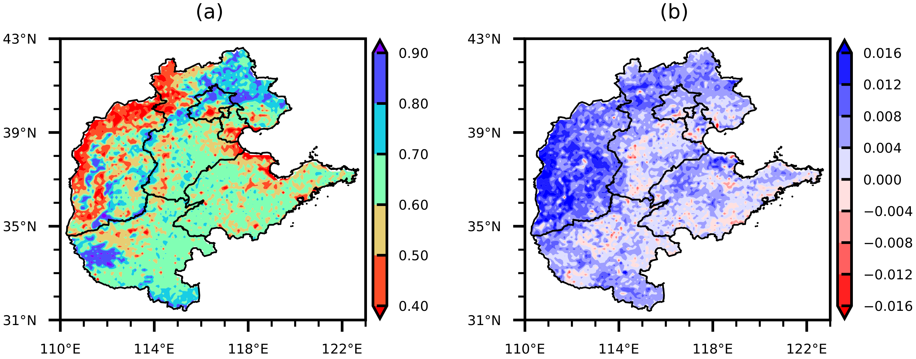
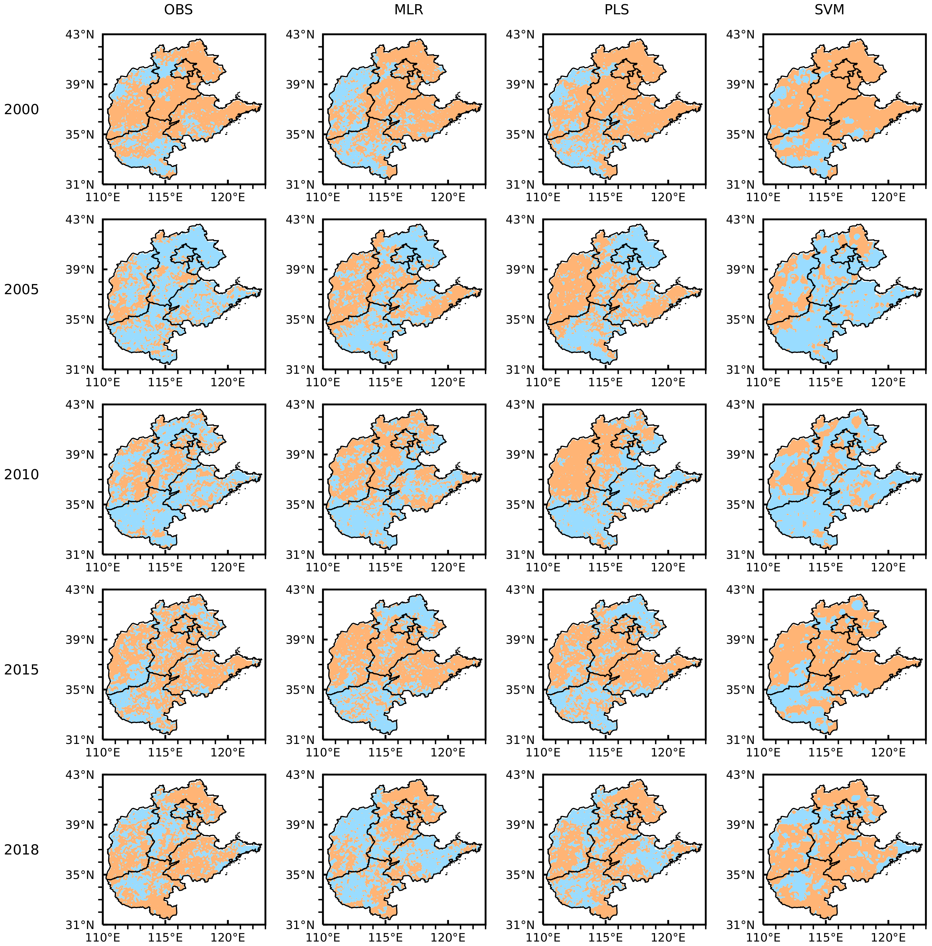
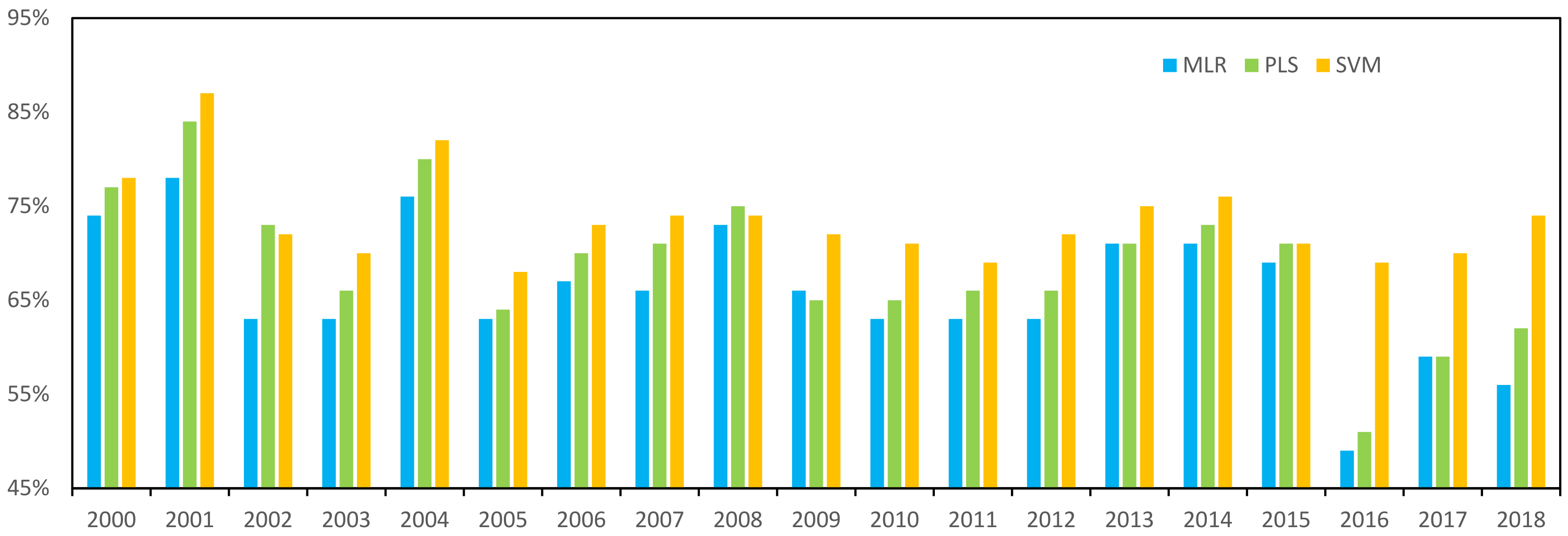
MEVC Model Simulation

We used three MEVC model to simulate vegetation coverage change in North China during 2000–2018. Figure 8 presents the observation and simulation results of vegetation coverage fluctuation in 2000, 2005, 2010, 2015, and 2018. In 2000, MLR simulates the area with increased vegetation coverage in Shanxi Province as a decrease. MLR and PLS simulate the area with increased vegetation coverage in Henan Province as a decrease. In 2005, MLR and PLS simulated error is quite large in Shanxi, and SVM simulated error north of Hebei. In 2010, PLS simulated error is quite large in Shanxi and Hebei, and the SVM is consistent in North China. In 2015, the three models’ simulation can well reproduce the observation. In 2018, MLR and PLS simulated error is quite large in Shandong. The linear model (MLR and PLS model) is higher for some sporadic point simulation, while the nonlinear model (SVM model) shows better performance for the overall trend simulation. In order to quantify and compare the simulation results of the three models during 2000 to 2018, the SAR between the observation and the model simulation is presented in Figure 9. In 2002 and 2015, the SAR of the SVM model was slightly lower than the PLS model; in 2009, 2013, and 2017, the SAR of the PLS model was lower than the MLR model. In 89% of these years, the SAR of the nonlinear model is better than the linear model. From the overall performance of the model, the nonlinear MEVC model is superior to the linear MEVC model. The MLR and PLS models are based on the linear hypothesis and do not consider the complexity of ecosystems and the nonlinearity of climate change on vegetation dynamic change. The SVM model can describe the complex nonlinear relationship between meteorology and the vegetation system.

4. Discussion

North China is the main wheat-producing base in northern China, and crop yields are closely related to climate change [41]. Consequently, predicting vegetation coverage change is an urgent problem in North China. In this study, the artificial intelligence model (SVM model) was driven by a station observation dataset. The MEVC SVM model showed better performance with regard to vegetation coverage change than the MLR and PLS models, using remotely sensed summer vegetation coverage data combined with meteorological elements of MJJ and JJA (Figure 8 and Figure 9). However, the artificial intelligence model gives higher error for some sporadic point simulations.

This paper develops an MEVC model based on the entire region of North China, without considering the differences of vegetation types. Studies have shown that grassland is closely related to precipitation, and farmland and forest are closely related to temperature [13,42]. Peng et al. [1] have shown that the vegetation dynamics trend of the Qinghai Tibet Plateau is affected by topography. There are a few studies that combine the Coupled Model Intercomparison Project 5 (CMIP5) to predict future vegetation changes [22,41].Consequently, we should collect related data, including topography and CMIP6, and combine machine learning methods to build a better vegetation prediction model.

Local climate and large-scale climatic conditions are the predictors of vegetation change [12,43]. EI Ninõ-Southern Oscillation (ENSO) has a significant impact on regional rainfall and temperature, which will affect the production of crops [44,45]. Future studies will use local climate, topography, and large-scale climate conditions, including ENSO, atmospheric circulation, and sea surface temperatures (SSTs) anomalies in key areas as predictors to predict the vegetation coverage change.

5. Conclusions

This paper analyzes the temporal and spatial characteristics of meteorological elements and vegetation coverage, determines the key meteorological elements affecting the change of vegetation coverage in North China, and develops an MEVC classification model utilizing the SVM methods. The obtained results are as follows: The climate has been changing to warm and dry state in North China during 2000–2018. Correlation analysis revealed that precipitation, relative humidity, and sunshine hours of JJA, as well as air temperature and ground temperature of MJJ, have close relationships with the interannual variation of summer vegetation coverage in North China. The MEVC classification model can well reproduce the change symbols of vegetation coverage in North China from 2000 to 2018. The mean SAR between observation and simulation is 70%, which shows that the MEVC classification model has good performance.

References

1. Peng, J.; Liu, Z.; Liu, Y.; Wu, J.; Han, Y. Trend analysis of vegetation dynamics in Qinghai-Tibet Plateau using Hurst Exponent. Ecol. Indic. 2012, 14, 28–39. [Google Scholar] [CrossRef]
2. Nemani, R.; Keeling, C.D.; Hashimoto, H.; Jolly, W.M.; Piper, S.C.; Tucker, C.J.; Myneni, R.B.; Running, S.W. Climate-Driven Increases in Global Terrestrial Net Primary Production from 1982 to 1999. Science 2003, 300, 1560–1563. [Google Scholar] [CrossRef] [PubMed] [Green Version]
3. Weiss, J.L.; Gutzler, D.S.; Allred Coonrod, J.E.; Dahm, C.N. Stomatal Conductance Characteristics of Populus euphrat ica Leaves and Response to Environmental Factors in the Extreme Arid Region. J. Arid Environ. 2004, 57, 507–534. [Google Scholar] [CrossRef]
4. Jiang, L.; Guli, J.; Bao, A.; Guo, H.; Ndayisaba, F. Vegetation dynamics and responses to climate change and human activities in Central Asia. Sci. Total Environ. 2017, 599–600, 967–980. [Google Scholar] [CrossRef] [PubMed]
5. Kong, D.; Zhang, Q.; Singh, V.; Shi, P. Seasonal vegetation response to climate change in the Northern Hemisphere (1982–2013). Glob. Planet. Chang. 2017, 148, 1–8. [Google Scholar] [CrossRef] [Green Version]
6. Hoffmann, W.; Jackson, R. Vegetation–Climate Feedbacks in the Conversion of Tropical Savanna to Grassland. J. Clim. 2000, 13, 1593–1602. [Google Scholar] [CrossRef]
7. Chaitra, A.; Upgupta, S.; Bhatta, L.; Mathangi, J.; Anitha, D.; Sindhu, K.; Kumar, V.; Agrawal, N.; Murthy, M.; Qamar, F.; et al. Impact of Climate Change on Vegetation Distribution and Net Primary Productivity of Forests of Himalayan River Basins: Brahmaputra, Koshi and Indus. Am. J. Clim. Chang. 2018, 7, 271–294. [Google Scholar] [CrossRef] [Green Version]
8. Gong, Z.; Zhao, S.; Gu, J. Correlation analysis between vegetation coverage and climate drought conditions in North China during 2001–2013. J. Geogr. Sci. 2016, 27, 143–160. [Google Scholar] [CrossRef]
9. Liu, F.; Qin, T.; Girma, A.; Wang, H.; Weng, B.; Yu, Z.; Wang, Z. Dynamics of Land-Use and Vegetation Change Using NDVI and Transfer Matrix: A Case Study of the Huaihe River Basin. Pol. J. Environ. Stud. 2018, 28, 213–223. [Google Scholar] [CrossRef]
10. Zhu, W.; Lei, H. Urban vegetation coverage monitoring technology based on NDVI. Adv. Eng. Res. 2018, 163, 1610–1618. [Google Scholar]
11. Wang, J.; Wang, K.; Zhang, M.; Zhang, C. Impacts of climate change and human activities on vegetation cover in hilly southern China. Ecol. Eng. 2015, 81, 451–461. [Google Scholar] [CrossRef]
12. Zhao, L.; Dai, A.; Dong, B. Changes in global vegetation activity and its driving factors during 1982–2013. Agric. For. Meteorol. 2018, 249, 198–209. [Google Scholar] [CrossRef]
13. Duo, A.; Zhao, W.; Qu, X.; Jing, R.; Xiong, K. Spatio-temporal variation of vegetation coverage and its response to climate change in North China plain in the last 33 years. Int. J. Appl. Earth Obs. 2016, 53, 103–117. [Google Scholar]
14. Li, P.; Hu, Z.; Liu, Y. Shift in the trend of browning in Southwestern Tibetan Plateau in the past two decades. Agric. For. Meteorol. 2020, 287, 107950. [Google Scholar] [CrossRef]
15. Shi, W.; Tao, F.; Zhang, Z. A review on statistical models for identifying climate contributions to crop yields. J. Geogr. Sci. 2013, 23, 567–576. [Google Scholar] [CrossRef]
16. Chen, C.; He, B.; Guo, L.; Zhang, Y.; Xie, X.; Chen, Z. Identifying Critical Climate Periods for Vegetation Growth in the Northern Hemisphere. J. Geophys. Res. Biogeosci. 2018, 123, 2541–2552. [Google Scholar] [CrossRef]
17. Lucht, W.; Prentice, I.C.; Myneni, R.B.; Sitch, S.; Friedlingstein, P.; Cramer, W.; Bousquet, P.; Buermann, W.; Smith, B. Climatic control of the high-latitude vegetation greening trend and Pinatubo effect. Science 2002, 296, 1687–1689. [Google Scholar] [CrossRef] [Green Version]
18. Peng, C. From static biogeographical model to dynamic global vegetation model: A global perspective on modelling vegetation dynamics. Ecol. Model. 2000, 135, 33–54. [Google Scholar] [CrossRef]
19. Fu, J.; Niu, J.; Sivakumar, B. Prediction of vegetation anomalies over an inland river basin in north-western China. Hydrol. Process. 2018, 32, 1814–1827. [Google Scholar] [CrossRef]
20. Martiny, N.; Philippon, N.; Richard, Y.; Camberlin, P.; Reason, C. Predictability of NDVI in semi-arid African regions. Theor. Appl. Climatol. 2010, 100, 467–484. [Google Scholar] [CrossRef]
21. Bai, H.; Gong, Z.; Sun, G.; Li, L.; Zhou, L. Study on the influence model of meteorological elements on summer vegetation coverage in North China(in Chinese). Chin. J. Atmos. Sci. 2022, 46, 27–39. (In Chinese) [Google Scholar]
22. Zheng, Y.; Han, J.; Huang, Y.; Fassnacht, S.; Xie, S.; Lv, E.; Chen, M. Vegetation response to climate conditions based on NDVI simulations using stepwise cluster analysis for the Three-River Headwaters region of China. Ecol. Indic. 2018, 92, 18–29. [Google Scholar] [CrossRef]
23. Shi, Y.; Jin, N.; Ma, X.; Wu, B.; He, Q.; Yue, C.; Yu, Q. Attribution of climate and human activities to vegetation change in China using machine learning techniques. Agric. For. Meteorol. 2020, 294, 108146. [Google Scholar] [CrossRef]
24. Lary, D.J.; Alavi, A.H.; Gandomi, A.H.; Walker, A.L. Machine learning in geosciences and remote sensing. Geosci. Front. 2016, 7, 3–10. [Google Scholar] [CrossRef] [Green Version]
25. Pal, M.; Maity, R.; Ratnam, J.; Nonaka, M.; Behera, S. Long-lead Prediction of ENSO Modoki Index using Machine Learning algorithms. Sci. Rep. 2020, 10, 365. [Google Scholar] [CrossRef]
26. Li, X.; Yuan, W.; Dong, W. A Machine Learning Method for Predicting Vegetation Indices in Chinas. Remote Sens. 2021, 13, 1147. [Google Scholar] [CrossRef]
27. Huang, J.; Ma, J.; Guan, X.; Li, Y.; He, Y. Progress in Semi-arid Climate Change Studies in China. Adv. Atmos. Sci. 2019, 36, 922–937. [Google Scholar] [CrossRef]
28. Huang, J.; Li, Y.; Fu, C.; Chen, F.; Fu, Q.; Dai, A.; Shinoda, M.; Ma, Z.; Guo, W.; Li, Z.; et al. Dryland climate change: Recent progress and challenges. Rev. Geophys. 2017, 55, 719–778. [Google Scholar] [CrossRef]
29. Cortes, C.; Vapnik, V. Support-vector networks. Mach. Learn. 1995, 20, 273–297. [Google Scholar] [CrossRef]
30. Rumpf, T.; Mahlein, A.; Steiner, U.; Oerke, E.; Dehne, H.; Plümer, L. Early detection and classification of plant diseases with Support Vector Machines based on hyperspectral reflectance. Comput. Electron. Agric. 2010, 74, 91–99. [Google Scholar] [CrossRef]
31. Wang, H. Partial Least-Squares Regression-Method and Applications; National Defense Industry Press: Beijing, China, 1999; pp. 200–210. (In Chinese) [Google Scholar]
32. Shawul, A.A.; Chakma, S.; Melesse, A.M. The response of water balance components to land cover change based on hydrologic modeling and partial least squares regression (PLSR) analysis in the Upper Awash Basin. J. Hydrol. Reg. Stud. 2019, 26, 100640. [Google Scholar] [CrossRef]
33. Wei, F. Modern Climate Statistical Analysis and Prediction Techniques; China Meteorological Press: Beijing, China, 1999; pp. 188–194. (In Chinese) [Google Scholar]
34. Vapnik, N. Statistical Learning Theory; Wiley: New York, NY, USA, 1998. [Google Scholar]
35. Duan, H.; Yan, C.; Tsunekawa, A.; Song, X.; Li, S.; Xie, J. Assessing vegetation dynamics in the Three-North Shelter Forest region of China using AVHRR NDVI data. Environ. Earth Sci. 2011, 64, 1011–1020. [Google Scholar] [CrossRef]
36. Zhang, Y.; Song, C.; Band, L.; Sun, G.; Li, J. Reanalysis of global terrestrial vegetation trends from MODIS products: Browning or greening. Remote Sens. Environ. 2017, 191, 145–155. [Google Scholar] [CrossRef] [Green Version]
37. Chen, C.; Park, T.; Wang, X.; Piao, S.; Xu, B.; Chaturvedi, R.K.; Fuchs, R.; Brovkin, V.; Ciais, P.; Fensholt, R.; et al. China and India lead in greening of the world through land-use management. Remote Sens. Environ. 2019, 191, 145–155. [Google Scholar]
38. Cui, L.; Shi, J. Temporal and spatial response of vegetation NDVI to temperature and precipitation in eastern China. J. Geogr. Sci. 2010, 20, 163–176. [Google Scholar] [CrossRef]
39. Wu, D.; Zhao, X.; Liang, S.; Zhou, T.; Huang, K.; Tang, B.; Zhao, W. Time-lag effects of global vegetation responses to climate change. Glob. Chang. Biol. 2015, 21, 3520–3531. [Google Scholar] [CrossRef]
40. Yuan, J.; Xu, Y.; Xiang, J.; Wu, L.; Wang, D. Spatiotemporal variation of vegetation coverage and its associated influence factor analysis in the Yangtze River Delta, eastern China. Environ. Sci. Pollut. Res. Int. 2019, 26, 32866–32879. [Google Scholar] [CrossRef]
41. Crane-Droesch, A. Machine learning methods for crop yield prediction and climate change impact assessment in agriculture. Environ. Res. Lett. 2018, 13, 114003. [Google Scholar] [CrossRef] [Green Version]
42. Qu, B.; Zhu, W.; Jia, S.; Lv, A. Spatio-Temporal Changes in Vegetation Activity and Its Driving Factors during the Growing Season in China from 1982 to 2011. Remote Sens. 2015, 384, 13729–13752. [Google Scholar] [CrossRef] [Green Version]
43. Ji, L.; Fan, K. Climate Prediction of Satellite-Based Spring Eurasian Vegetation Index (NDVI) using Coupled Singular Value Decomposition (SVD) Patterns. Remote Sens. 2019, 11, 2123. [Google Scholar] [CrossRef] [Green Version]
44. Liu, Y.; Yang, X.; Wang, E.; Xue, C. Climate and crop yields impacted by ENSO episodes on the North China Plain: 1956–2006. Reg. Environ. Chang. 2014, 14, 49–59. [Google Scholar] [CrossRef] [Green Version]
45. Stone, R.C.; Marcussen, T.; Hammer, G.L. Prediction of global rainfall probabilities using phases of the Southern Oscillation Index. Nature 1996, 384, 252–255. [Google Scholar] [CrossRef]
Figure 1. Study workflow.
Remotesensing 14 01307 g001
Figure 2. The location of study area and distribution of meteorological observation stations.
Remotesensing 14 01307 g002
Figure 3. Special distribution basic characteristics of meteorological elements in North China during 2000–2018: (a1e1) are the averaged climatic values of air temperature (unit: C), precipitation (unit: mm), relative humidity (unit: %), sunshine hours (unit: h), and ground temperature (unit: C) in summer, respectively; (a2e2) are the linear trend coefficients.
Remotesensing 14 01307 g003
Figure 4. Basic characteristics of summer vegetation coverage (dimensionless) in North China during 2000–2018. (a) Mean value; (b) linear trend coefficients.
Remotesensing 14 01307 g004
Figure 5. Correlation coefficients between summer vegetation coverage and meteorological elements (temperature (T), precipitation (P), relative humidity (R), sunshine hours (S), and ground temperature (G)) in different periods (JJA: June–August, MJJ: May–July, AMJ: April–June, and MAM: March–May). The blue dotted line indicates the 95% significance level, and the red dotted line indicates the 99% significance level.
Remotesensing 14 01307 g005
Figure 6. Heat map of correlation coefficient between vegetation coverage ( V C R ) and meteorological elements (temperature (T), precipitation (P), relative humidity (R), sunshine hours (S), and ground temperature (G)).
Remotesensing 14 01307 g006
Figure 7. Parameter sensitivity analysis.
Remotesensing 14 01307 g007
Figure 8. Observation and simulation map of positive and negative fluctuation anomaly of vegetation coverage for 2000, 2005, 2010, 2015, and 2018 in North China (among them, the first column is the observation diagram, and the second, third, and fourth columns are the simulation diagrams of the MLR model, the PLS model, and the SVM model, respectively). Blue and orange indicate positive and negative vegetation coverage anomaly, respectively.
Remotesensing 14 01307 g008
Figure 9. SAR of vegetation coverage anomaly during 2000–2018.
Remotesensing 14 01307 g009
Publisher’s Note: MDPI stays neutral with regard to jurisdictional claims in published maps and institutional affiliations.