Article

Relationship between the Intraseasonal Oscillation over Mid-High-Latitude Eurasia and the Stratospheric Sudden Warming Event in February 2018

1
Key Laboratory of Meteorological Disaster, Ministry of Education (KLME)/Joint International Research Laboratory of Climate and Environmental Change (ILCEC)/Collaborative Innovation Center on Forecast and Evaluation of Meteorological Disasters (CIC-FEMD), Nanjing University of Information Science and Technology, Nanjing 210044, China
2
International Pacific Research Center, Department of Atmospheric Sciences, University of Hawaii at Manoa, Honolulu, HI 96822, USA
*
Author to whom correspondence should be addressed.
These authors contributed equally to this work.
Remote Sens. 2022, 14(8), 1873; https://doi.org/10.3390/rs14081873
Submission received: 22 February 2022 / Revised: 2 April 2022 / Accepted: 11 April 2022 / Published: 13 April 2022

Abstract

:
Taking the stratospheric sudden warming (SSW) event in February 2018 as an example, the relationship between the SSW event and the intraseasonal oscillation (ISO) mode over mid-high-latitude Eurasia is investigated by daily reanalysis data. First, the 2018 SSW event and mid-high-latitude ISO are reviewed. The 2018 SSW event is a typical vortex-split event defined by the NCEP-DOE dataset, and the ISO mode features a southeastward propagation. Along with the ISO propagation, temperature anomalies developed from troposphere to stratosphere in the 2018 wintertime. It is also found that a strong ISO event occurred before the onset of SSW in this wintertime. Our analysis reveals that the correlation is significant when mid-high-latitude ISO leads the 2018 SSW event by 9–13 days. Occurrence of strong ISO 9–13 days before the SSW event is found to be conducive to its onset. The diagnosis of planetary wave activity indicates that stronger ISO leads to strengthened wavenumber-2 geopotential height anomalies; then, its in-phase superposition of climatological geopotential height makes up for the upward-propagating tropospheric planetary waves, which is in favor of the onset of the 2018 SSW event. The outcome of energy conversion equations also reveals that ISO perturbation contributes to the onset of SSW. Lastly, the contribution of the vertical component of Plumb wave activity flux propagated upward from the region of mid-high-latitude ISO is estimated at approximately 69%.

1. Introduction

Stratospheric sudden warming (SSW) events occur in the winter stratosphere of both hemispheres, featuring a shift or a breakdown of the polar vortex [1]. The onset of SSW is usually accompanied by a sharp increase of temperature and a reversal of zonal wind direction (westerlies turning into easterlies) in the polar stratosphere [2]. The occurrence frequency of SSW events in the Northern Hemisphere is approximately six times per decade so far. Since the discovery of SSW [3], it has attracted wide attention, including its classification [1,4], mechanism [5], and its prediction by models [6,7]. A series of studies have demonstrated that several factors can influence SSW events, such as Quasi-Biennial Oscillation (QBO), El Nino-Southern Oscillation (ENSO), and Madden-Julian Oscillation (MJO) [8,9,10,11,12,13].
The MJO is the most dominant mode of tropical intraseasonal oscillation, which mainly exhibits eastward propagation during northern winter [14]. Previous studies have revealed that SSW events have connections with MJO on both intraseasonal and interannual timescales. Garfinkel et al. [15] firstly figured out the lag relationship between SSW events and the MJO. They pointed out that SSW events tend to occur after a certain MJO phase. Garfinkel et al. [16] further indicated that MJO phase 7 (defined by Wheeler and Hendon [17]) leads to a North Pacific low and then a weakened polar vortex, which favors the onset of SSW, while MJO phase 3 plays an opposite role. Ma et al. [12] showed that the MJO–SSW relationship can be modulated by ENSO. In addition, Wang et al. [18] discussed the link between the frequency of MJO phases and the interannual variability of stratospheric wave activity (SSW is a phenomenon of the extremely strong stratospheric wave activity) in the Northern Hemisphere. Overall, the MJO–SSW connection has been verified.
The atmospheric intraseasonal variability exists not only in the tropical region, but also in mid-high latitudes [19]. Some studies have shown that the intraseasonal oscillation (ISO) exists over mid-high-latitude Eurasia region, and that it greatly impacts extratropic circulation. Yang et al. [20] showed that the ISO signal has a feature of evidently southeastward propagation during boreal winter and is closely related to the Eurasia teleconnection pattern (EU). Then, Yang and Li [21] put forward the detailed ISO mode over mid-high-latitude Eurasia, which has southeastward propagation for both the temperature anomaly and geopotential height anomaly in the whole troposphere. They pointed out that the southeastward movement of temperature anomaly and geopotential height anomaly are induced by the ISO-mean flow interaction and Rossby wave energy propagation originating at the high latitude Europe/Atlantic sector. Subsequently, Yang and Li [22,23] found that mid-high-latitude ISO plays a vital role in regulating high-latitude blockings (Pacific blocking and Okhotsk blocking). Nonetheless, these existing studies on mid-high-latitude ISO in Eurasia only focus on the tropospheric circulation; less is known about its linkage with the stratospheric circulation. Does mid-high-latitude ISO have any relevance to SSW? The ISO–SSW relationship has not been explored thoroughly.
Cohen et al. [24,25] pointed out that the Eurasian sector is a significant source region of planetary waves, where these waves can propagate from troposphere to stratosphere. They believed that these upward-propagating waves will induce SSW events. Therefore, SSW events are closely related to the Eurasian continent. Our preliminary study showed that there exists a significant lead–lag correlation between SSW and the ISO of surface air temperature, which suggests a possible cause–effect relation between them. The primary objective of the manuscript is to investigate the potential connection between them. Therefore, taking the specific year of 2018 as an example, when a typical SSW event occurred, the linkage between mid-high-latitude ISO and SSW is revealed.
The remainder of this article is organized in the following manner. Reanalysis dataset and methods used in this paper are described in Section 2. In Section 3, both the mid-high-latitude ISO and 2018 SSW event are briefly introduced, respectively, and then the relationship between them is presented in detail. Discussions and primary conclusions are given in Section 4 and Section 5, respectively.

2. Data and Methods

2.1. Data

Daily reanalysis data provided by the National Centers for Environmental Prediction—Department of Energy (NCEP-DOE) [26] from 1979 to 2018 is used in this study. The dataset includes the variables of temperature T, zonal wind u, meridional wind v and geopotential height Z at 17 pressure levels (1000, 925, 850, 700, 600, 500, 400, 300, 250, 200, 150, 100, 70, 50, 30, 20, and 10 hPa). Additionally, we use the temperature at the σ = 0.995 level as a proxy for the surface air temperature (SAT). This is obtained from the National Centers for Environment Prediction—National Center for Atmospheric Research (NCEP-NCAR) reanalysis data [27]. NCEP-NCAR and NCEP-DOE reanalysis data employed in this paper have the same horizontal resolution of 2.5° × 2.5°. Also, it is worth mentioning that the results are not sensitive to the reanalysis data chosen.

2.2. Methods

In this study, we mainly focus on the relationship between ISO and SSW on the intraseasonal timescale. To capture the intraseasonal signals, firstly, the mean and first four harmonics of the annual cycle were removed from the reanalysis data. Secondly, the so-derived data was subjected to a band-pass (10–60-day) filter by fast Fourier transform (FFT). Then, only the wintertime period of these data were selected for the following analysis. Here, the wintertime is defined as the period from 1 December to 31 March, removing 29 February. The effective degree of freedom was estimated based on Alaka et al. [28].
The most prominent mode of ISO extracted from SAT over mid-high-latitude Eurasia (20°–140°E, 35°–80°N) during boreal winter was put forward by Yang and Li [21]. They suggested that the statistically significant ISO signal appears at a period of 10–60 days. This ISO mode is further divided into eight phases by the first two principal components (PC1 and PC2) of EOF in Cui et al. [29]. Referring to this method, PC1 and PC2 are used in this study to represent the mid-high-latitude ISO. PC1 and PC2 time series for 2018 wintertime can be achieved in two ways: one is extracting the PC index of 2018 winter direct from EOF analysis, the other is projecting intraseasonal SAT anomalies of 2018 wintertime onto EOF1 and EOF2. Note that the consequences obtained by these two methods are highly consistent. Here, we apply the former method in the follow-up study. Additionally, the amplitude of ISO is defined as PC 1 2 + PC 2 2 , where only the ISO with amplitudes over 1.0 are denoted as strong ISO.
The 2018 SSW event is identified by the World Meteorology Organization (WMO) definition of SSW events [1]; that is, the zonal mean zonal winds at 60°N and 10 hPa reverse from westerlies to easterlies, and the 10 hPa zonal mean temperature gradient between 60°N and 90°N reverses from negative to positive. SSW events are induced by the upward propagation of planetary waves from troposphere to stratosphere [30]. The amplitude of these planetary waves increases with height, and these waves irreversibly break and release energy until reaching a certain height [31]. The propagating direction of these waves is characterized by Eliassen–Palm (EP) flux [32] in the meridional–pressure plane. The horizontal component of EP flux represents eddy momentum flux, while the vertical component denotes eddy heat flux. EP flux divergence was calculated to measure the interaction between upward propagating planetary waves and the mean flows [33]. The negative flux divergence reflects easterly forcing on the mean flow, which is in favor of the onset of SSW events. The formulas of EP flux and flux divergence are written as follows [32]:
F φ = a ( c o s φ ) u v ¯ ,
F p = a ( c o s φ ) f v θ ¯ θ p ¯ ,
  F = 1 a   c o s φ ( F φ c o s φ ) φ + F p p ,
where F φ represents the horizontal component of EP flux; F P represents the vertical component of EP flux;   F denotes the divergence of EP flux; a is the radius of the Earth; φ is the latitude (in radians); u is the zonal wind; v is the meridional wind; f is the Coriolis parameter; θ denotes potential temperature; and the overbar and prime indicate zonal mean and zonal anomaly, respectively.
As EP flux and its divergence are zonal mean quantities, we also apply three-dimensional Plumb [34] wave activity flux to diagnose the planetary wave propagation for specific mid-high-latitude Eurasian sectors. Referring to Shi et al. [35], the formulas of Plumb wave activity flux is obtained as follows:
F p l u m b x = p p 0 c o s φ · v g 2 1 2 Ω a s i n 2 φ ( v g Φ ) λ ,
F p l u m b y = p p 0 c o s φ · u g v g + 1 2 Ω a s i n 2 φ ( u g Φ ) λ ,
F p l u m b z = p p 0 c o s φ · f S v g T 1 2 Ω a s i n 2 φ ( T Φ ) λ ,
where F p l u m b x , F p l u m b y , and F p l u m b z correspond to the zonal, meridional, and vertical components of Plumb wave activity flux, respectively; p 0 is the standard reference pressure; S ,   Ω ,     λ ,   Φ represent the static stability, the rotation speed of the Earth, the longitude (in radians), and the geopotential, respectively; u g and v g are geostrophic winds; and the overbar, prime, and remaining parameters are the same as those in the EP flux formula.
To investigate the mechanism of the ISO–SSW relationship from the view of energy conversion, the barotropic kinetic energy conversion and baroclinic available potential energy conversion equations are applied in this research. Referring to Du and Lu [36], the two energy conversion equations are expressed as follows:
C P = f S ( v T u ¯ p u T v ¯ p ) ,
C K = v 2 u 2 2 ( u ¯ x v ¯ y ) u v ( u ¯ y + v ¯ x ) .
where CP represents baroclinic available potential energy conversion between mean flow and intraseasonal disturbances, CK denotes barotropic kinetic energy between mean flow and intraseasonal disturbances, the prime indicates intraseasonal perturbation, and the overbar indicates the wintertime mean state during 1979–2018. The positive value means energy conversion from the mean flow to the intraseasonal perturbation.

3. Results

In order to achieve a better understanding of the relationship between the 2018 SSW and mid-high-latitude ISO, we firstly take an overview of the 2018 SSW event and mid-high-latitude ISO.

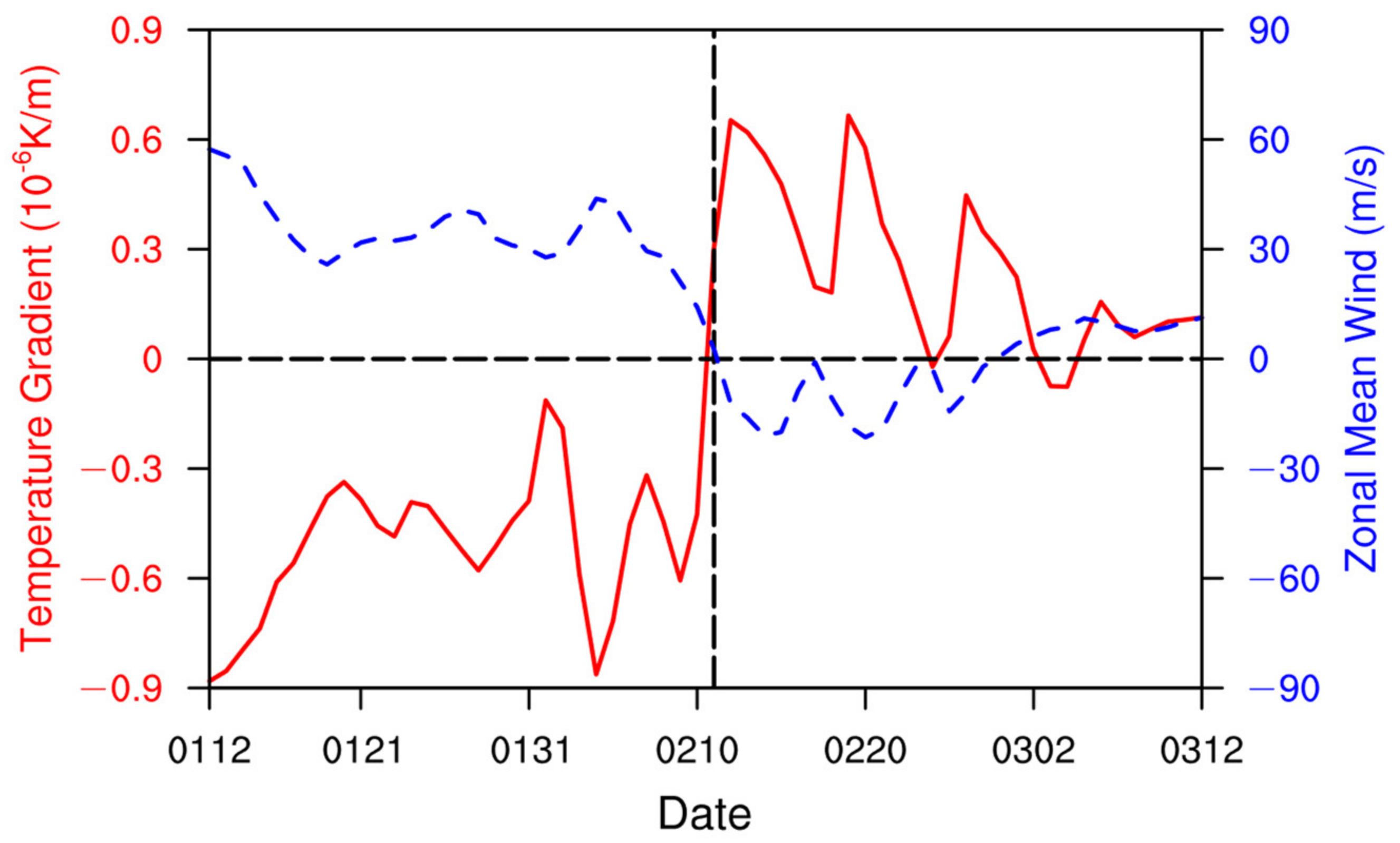
3.1. Overview of 2018 SSW Event

The 2018 SSW event, a recent typical major event, has been significantly documented [37,38,39]. For brevity, only the onset date and the classification of this event will be shown in this subsection.
The evolutions of the 10 hPa zonal mean wind at 60°N and the 10 hPa temperature gradient between 60°N and the North Pole are shown in Figure 1. It can be found that the zonal mean wind turned from westerly to easterly wind on 11 February, and the zonal mean temperature gradient changed from negative to positive 1 day before. Consequently, in accordance with the WMO definition of SSW events, the onset date of this event is redefined as 11 February.
According to the variation of polar vortex, SSW events can be further classified into two categories: vortex-displacement events and vortex-split events [1]. To achieve an overview of this event type, the patterns of geopotential height at 500 hPa and 10 hPa during two sub-periods are displayed in Figure 2. During 2–4 February, the polar vortex was maintained at the North Pole, whether at 500 hPa or 10 hPa (Figure 2a,c). During 9–11 February, two anticyclones over the Aleutian and Atlantic sectors induced the vortex to split (Figure 2b,d). Therefore, the 2018 SSW belongs to a typical vortex-split event.
Furthermore, displacement SSW events are believed to be caused by wavenumber 1 (hereafter wave 1), while split events are induced by wavenumber 2 (hereafter wave 2) [40]. Shown in Figure 3 is the variation of wave-1 and wave-2 vertical components of EP flux and flux divergence. We can see that approaching the onset date of SSW, the vertical component of EP flux of wave 2 reached its maximum value, and the EP flux divergence of wave 2 reached its minimum value. However, the wave 1 component just fluctuates around zero. In other words, the upward propagation of wave 2 leads to this SSW event.
From the diagnosis above, the 2018 SSW event can be identified as a typical vortex-split warming event which was caused by wave 2. This is consistent with previous conclusions.

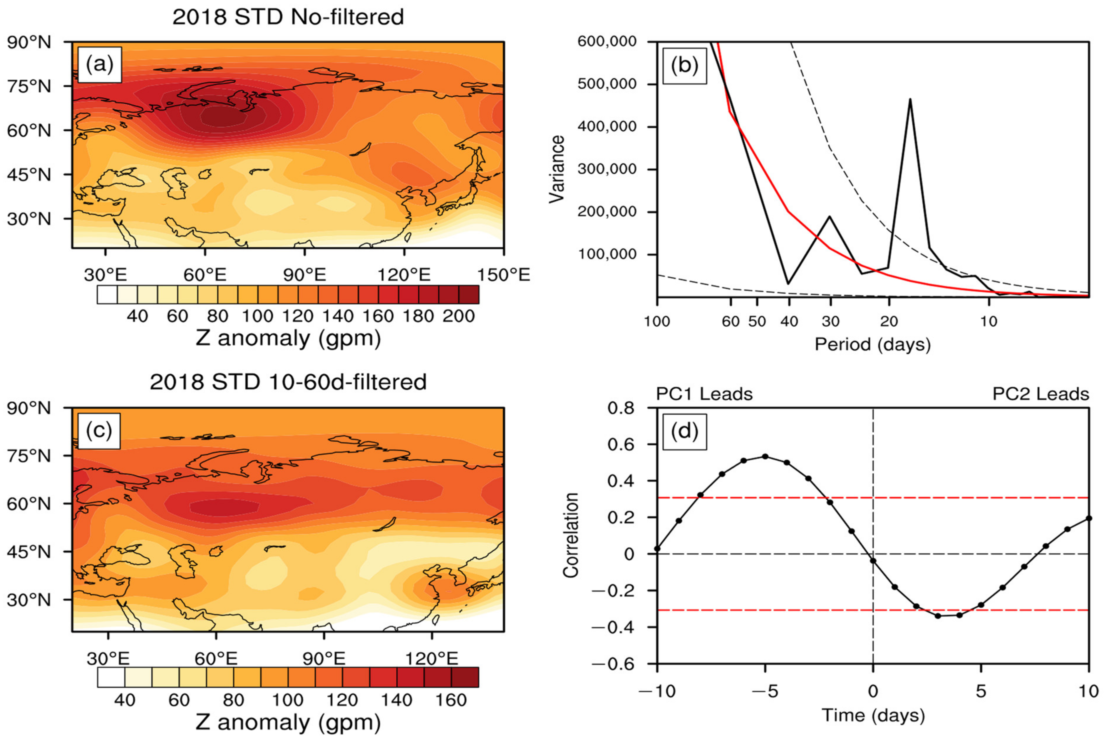
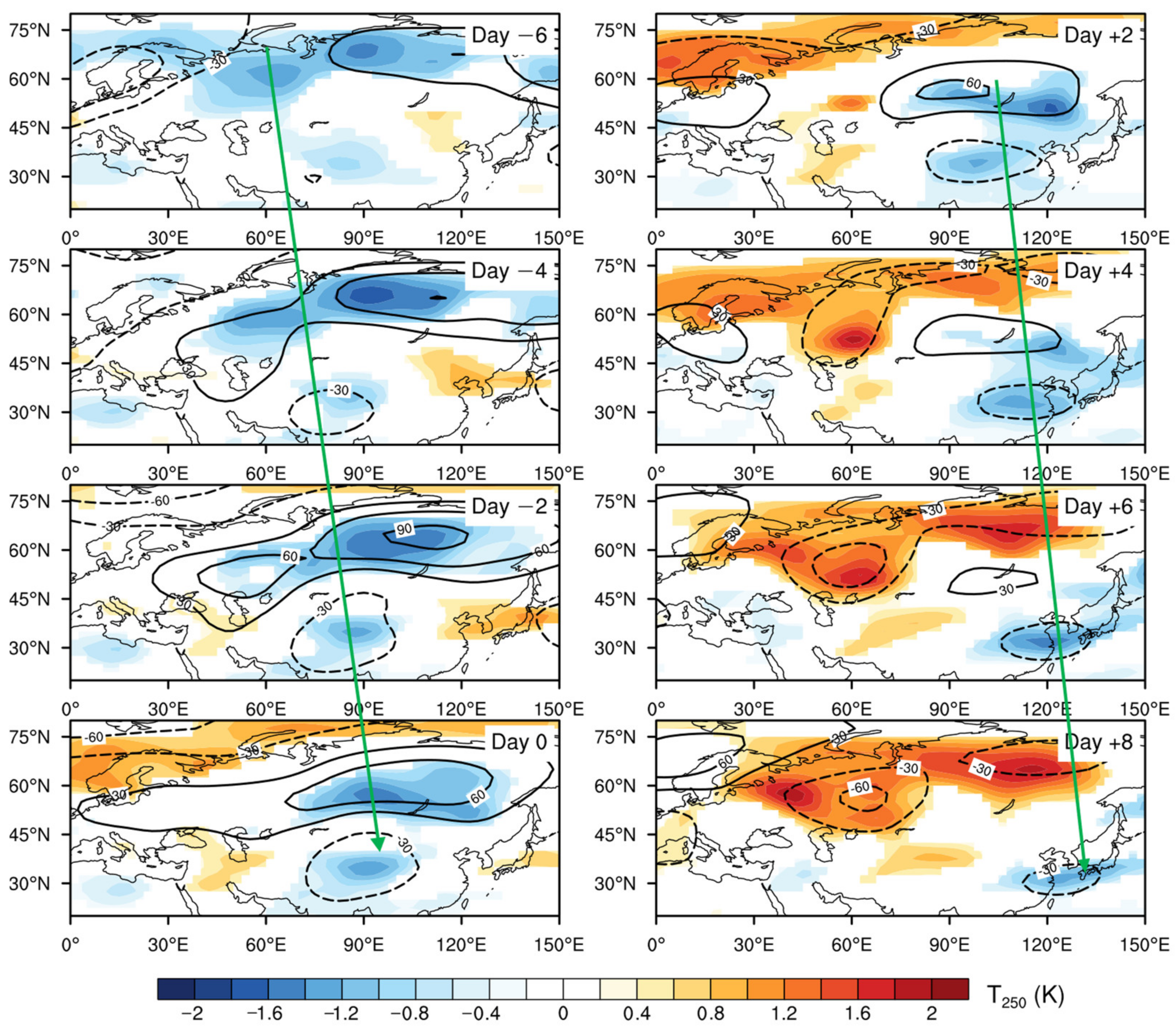
3.2. Signal of ISO over Mid-High-Latitude Eurasia

SSW events have been demonstrated to be controlled by forcing waves near the tropopause [41]. We first extract the main periodicity of tropopause geopotential height to confirm that the period of waves which could modulate the SSW event in 2018 is consistent with the period of mid-high-latitude ISO. Figure 4a shows the standard deviation (STD) of non-filtered geopotential height at 250 hPa over mid-high-latitude Eurasia during the 2018 wintertime. It can be seen that the largest STD appears at the 50°–80°N region. It should be mentioned that this region is also where the planetary waves propagate upwards most actively. Next, the maximum perturbation center near the Kara Sea (50°–70°N, 40°–80°E) is chosen for the power spectral analysis. The significant variability of this particular year is found to be on the timescale of 10–20 days, which is included in the period of 10–60 days (Figure 4b). When we focus on the timescale of ISO, the center of STD near the Kara Sea can still be captured (Figure 4c). There is a significant positive correlation coefficient when PC1 leads PC2 by 5 days and a significant negative correlation when PC2 leads PC1 by 3–4 days (Figure 4d). Both the power spectral analysis and lead–lag correlation of PC1 and PC2 indicate that, in this particular year, the quasi-biweekly scale of waves plays a more important role.
The propagation feature of the ISO of SAT over mid-high-latitude Eurasia has been described in great detail in both Yang and Li [21] and Cui et al. [29]. That is, the SAT anomalies are coupled with upper-tropospheric geopotential height, and temperature anomalies propagate southeastward. The same is true in the year of 2018. Figure 5 displays the evolution of the geopotential height and the temperature anomalies at 250 hPa in 2018. The negative geopotential height anomalies originating from high latitudes show a southeastward propagation. The anomalies propagate southeastward from Novaya Zemlya (60°E, 75°N) (Day −6) to East China (110°E, 40°N) (Day +8). One may notice that a secondary minima of temperature anomalies around (40°N, 90°E) is associated with negative geopotential height anomalies, while the other temperature minima around (60°N, 90°E) is associated with positive geopotential height anomalies. The reason why the same sign of temperature anomaly corresponding to different signs of geopotential height anomaly is due to the vertical profiles of temperature and geopotential height anomalies. The vertical profile shows a lower-cold upper-warm temperature anomaly, with a zero line near 150 hPa and a negative geopotential height anomaly at the whole troposphere at lower latitudes (around 40°N). The situation near the region of (60°N, 90°E) is a lower-cold upper-warm anomaly, with a zero line near 300 hPa and a positive geopotential height anomaly at the whole troposphere. Therefore, at 250 hPa, a cold anomaly is associated with a negative geopotential height anomaly near (40°N, 90°E), and a cold anomaly is associated with a positive geopotential height anomaly near (60°N, 90°E).
Figure 6 shows the meridional vertical cross sections of the 10–60-day filtered geopotential height anomaly and temperature anomaly averaged from 20°E to 140°E from Day −6 to Day +8, obtained by regressed geopotential height anomalies and temperature anomalies at all pressure levels on PC1 of the 2018 wintertime. The vertical distribution shows a hydrostatic relationship. For instance, a warm temperature center at a lower layer corresponds to a cold center at a higher layer, along with positive geopotential height anomaly existing in the whole troposphere at Day −2 around 60°N. This can be deemed as a connection between the ISO and the stratospheric temperature. Moreover, it is interesting to find that temperature anomalies reveal an evident signal of upward development in conjunction with the movement of ISO anomalies. Hence, in the year 2018, the ISO over the mid-high-latitude Eurasian region may be a precursor of the stratospheric temperature.
To summarize, we can find an upward propagation of temperature anomalies from troposphere to stratosphere in the 2018 wintertime, which is associated with mid-high-latitude ISO. This indicates that the 2018 SSW is related to the mid-high-latitude ISO. The following explores the exclusive connection between the SSW and mid-high-latitude ISO in 2018.

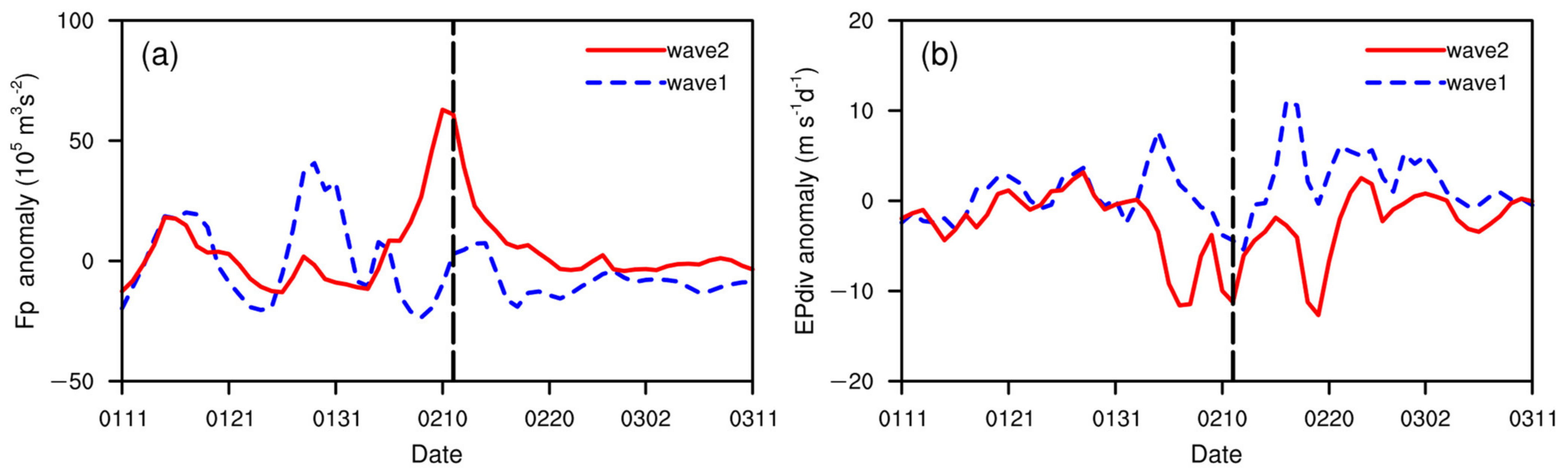
3.3. Relationship between the 2018 SSW Event and Mid-High-Latitude ISO

To further analyze the linkage between the mid-high-latitude ISO and the 2018 SSW event, the specific ISO during the 2018 winter is assessed. The evolution of ISO and its amplitude from 1 December 2017 to 31 March 2018 is illustrated in Figure 7. A complete strong ISO lifecycle (hereafter the strong ISO event) can be found before the onset day (11 February) of the 2018 SSW event, which started at 14 January. Therefore, we consider that this SSW event is associated with the amplitude of ISO.
With the intention of verifying our conjecture, a series of correlation analysis was carried out to investigate the statistical linkage between the 2018 SSW event and mid-high-latitude ISO. EP flux divergence is chosen to denote the SSW event, and PC index (a general designation of PC1, PC2, and the amplitude of ISO) is employed to represent mid-high-latitude ISO. Here, PC1 and PC2 indicate the first two principal components of the first two EOF modes, respectively, and the amplitude of ISO is defined as PC 1 2 + PC 2 2 . In the first step, we calculated the simultaneous correlation coefficient between EP flux divergence time series of the 2018 wintertime and PC1, between this divergence and PC2, and also between this divergence and amplitude of PC time series of 2018, respectively (not shown). The consequences show that none of the correlations are significant, which implies that there is no obvious in-phase or anti-phase correlation between the 2018 SSW event and mid-high-latitude ISO.
Since Figure 7 shows a strong ISO event prior to the onset of SSW, and as documented in Cohen et al. [24], an offset may exist between a tropospheric event and a stratospheric event due to the multiple-week timescale of stratosphere–troposphere interaction. Wondering whether a lead–lag correlation exists between the SSW and mid-high-latitude ISO or not, we applied a lead–lag correlation analysis on the EP flux divergence and the time series of PC index, especially the amplitude of ISO. As a result, the lead–lag correlation between this event and PC index is not significant during a long period, i.e., the entire 2018 wintertime (figure omitted). However, when we only pay attention to a short period, i.e., about 1 month centered on the onset day of the 2018 SSW event, significant correlations at the 0.05 significant level can be found (Figure 8). The significant correlation appears when the amplitude of ISO leads EP flux divergence by around 9–13 days, with the maximum correlation coefficient occurring at 11 days. This means that mid-high-latitude ISO can affect the SSW event. Specifically, the stronger the ISO 11 days before the onset day, the more conducive it is to its onset. A possible mechanism of this relationship will be discussed later. Also, the correlation when SSW leads ISO is not significant, though a sub-peak occurs when EP flux divergence leads the amplitude of ISO by about 7 days. This implies that an impact of SSW events on mid-high-latitude ISO exists, but it is not statistically significant in this year.
Consequently, we mainly focus on the impact of mid-high-latitude ISO on the 2018 SSW event in this study. We further corroborate the timescale of the relationship between ISO and SSW by wave–flow interaction (i.e., EP flux and its divergence). Figure 7 demonstrates a complete strong ISO event, and Figure 9 displays the evolution of EP flux and its divergence from the first day of this strong ISO event (14 January, i.e., lag −28) to the onset day of the SSW event (11 February, i.e., lag 0), with an interval of 2 days. From Figure 9, we can see that negative EP divergence transforms to positive EP divergence in the stratosphere from lag −28 to lag −24. During the period of from lag −22 to lag −14, the EP divergence remains weakly positive in the stratosphere, with EP flux convergence appearing at about 300 hPa. Then, from lag −12, the stratospheric EP flux divergence increases and further transforms into convergence until the onset of the SSW event. Note that this evolution of EP flux divergence can also be found in Figure 3b if we add the wave 1 and wave 2 components together. As mentioned in Section 2, EP flux convergence means easterly forcing. Therefore, the feature which occurred after lag −14 satisfied the condition for the onset of the SSW, i.e., zonal mean wind turns from strong westerly to easterly. This timescale is almost consistent with that of the significant lead–lag correlation.
Based on the above analysis, the impact of ISO on SSW is corroborated. Next, we will discuss the mechanism of the ISO-SSW relationship from the viewpoint of linear interference and energy conversion, respectively.
Garfinkel et al. [35] proposed a linear interference mechanism; that is, when the geopotential height anomalies are in phase with climatological planetary waves, it will favor the upward propagation of planetary waves. This has been affirmed by many studies [18,42,43]. We use this linear interference mechanism to detect how the 2018 SSW event is affected by mid-high-latitude ISO. Since the 2018 SSW event was induced by wave 2, and the geopotential height anomalies regressed on PC1 also present distribution of 2 waves roughly (not shown), we only present the evolution of wave 2 geopotential height. Depicted in Figure 10 is the variation of wave 2 geopotential height anomalies overlaid on the wave 2 climatological geopotential height from the first date of the strong ISO event to the onset date of the SSW event. The wave 2 climatological geopotential height barely changes, while the wave 2 geopotential height anomaly shows a southeastward movement. During the period from lag −28 to lag −16, there is a process of gradual anti-phase superposition of the geopotential height anomalies and climatological geopotential height. Then, the in-phase superposition of geopotential height anomalies and climatological geopotential height starts at lag −14. From lag −14 to lag −8, the height anomaly strengthens, with little variation of its location at mid-high latitudes. Then, the anomaly center starts moving southeastwardly, leading to the enhancement of in-phase overlay, which further favors the upward propagation of planetary waves. Owing to continuous southeastward propagation, the anomaly center gradually moves out of the climatological center after lag −4. Finally, the pattern of anomalies and climatological pattern are orthogonal at the onset day.
In addition to the overlay of 10–60-day filtered wave 2 geopotential height anomalies and climatological geopotential height at 250 hPa, we also present the longitude–height cross sections and latitude–height cross sections from lag −28 to lag 0 in Figure 11. We can see that the 10–60-day filtered geopotential height anomalies present obvious upward movement except for the southward and eastward movement in Figure 11a,b. From lag −28 to lag −16, the anti-phase superposition strengthens in the troposphere with the southward and eastward movement of geopotential height anomalies. Along with the upward movement of the anomaly fields, the anti-phase superposition also moves upward. From lag −14, the in-phase superposition of geopotential height anomaly strengthens in the troposphere, and moves upward after lag −8.
The above diagnosis of Figure 10 and Figure 11 gives us a better understanding of why a stronger mid-high-latitude ISO occurring 9–13 days before the onset of SSW is more conducive to its onset. Generally, stronger mid-high-latitude ISO corresponds to stronger height anomalies; the in-phase superposition of wave-2 geopotential height anomalies and climatological geopotential height started enhancing at the period from lag −13 to lag −9. Then, along with the southeastward and upward movement, the enhancement of in-phase superposition of wave 2 geopotential height anomalies and climatological geopotential height also moved upwards. This caused tropospheric planetary waves to become more active and propagate into stratosphere, which does a favor to the onset of this SSW event.
Above, we analyzed the mechanism of ISO-SSW relationship by using the linear interference mechanism. Next, we analyze the mechanism of the ISO–SSW relationship by using energy conversion equations. The results are shown in Figure 12. For examining the impact of ISO disturbance on the onset of SSW, we choose 50 hPa to represent the state of stratosphere, and focus on the polar region (60°–87.5°N, 0°–360°) from lag −28 to lag 0. It is revealed that before the onset date of the SSW, especially after lag −14, the ISO flow gains energy from the mean flow and contributes to the onset of SSW. Specifically, the ISO flow gains more barotropic kinetic energy before lag −9, while it gains more baroclinic available potential energy after lag −9. The results of energy conversion confirm that ISO did make a significant contribution to the onset of the SSW.
Ultimately, we are going to concentrate on the contribution of ISO from the mid-high-latitude Eurasian region to the SSW event. As plotted in Figure 13, the propagation of planetary waves over the Eurasian region is attained by Plumb wave activity flux along 20°–140°E from lag −28 (28 days before the onset of SSW) to lag 0 (the onset day of the SSW event). According to this figure, the characteristics of the propagation of Plumb wave flux are in accordance with the development of overlay of wave 2 geopotential height anomalies and climatological geopotential height. During the anti-phase period (lag −28 to −16), the downward Plumb flux developed, which was entirely not favorable for the onset of SSW. From lag −14, the in-phase superposition started. This leads to strong planetary waves which keep propagating from the troposphere into the stratosphere, contributing to the onset of SSW. Combining Figure 11 and Figure 13, the reason why the correlation coefficient is only significant from −9 to −13 can be found. That is, the anti-phase superposition caused planetary waves to accumulate in the troposphere. Hence, at the start of the in-phase, i.e., from −13 to −9 days, the strongest planetary waves propagate upward to the stratosphere, which makes the correlation coefficient significant during this period.
Using the vertical component of Plumb wave activity flux ( F p l u m b z ), the provision of mid-high-latitude ISO over the Eurasia region to the onset of the 2018 SSW event is estimated as follows:
rate = F φ i s o F φ a l l ,
where F φ i s o symbolizes the 10–60-day filtered upward-propagating F p l u m b z over the region of ISO mode (35°–80°N, 20°–140°E), and F φ all indicates the 10–60-day filtered upward-propagating F p l u m b z for the whole globe (35°–80°N, 0°–360°). We choose 15 days before the SSW onset day, i.e., lag −14 to lag 0, when the planetary waves continued propagating from the troposphere to stratosphere. The result is an average of 15 days, 35–80°N at 100 hPa. It is estimated that the 10–60-day filtered upward-propagating vertical component of Plumb wave activity flux emitted from the mid-high-latitude ISO region accounts for about 69% of that emitted that from the whole Northern Hemisphere. As illustrated in Figure 14, mid-high-latitude Eurasia is truly the main center of upward-propagating planetary waves, along with another weak upward-propagating center located in the North Pacific.

4. Discussion

In this research, the relationship between a single SSW event and ISO over mid-high latitude Eurasia is confirmed. This case study can give us a simple view of the potential linkage between the mid-high-latitude ISO and the SSW. The connections between the single SSW event and the ISO over mid-high latitude Eurasia are raised through this case study; nonetheless, whether the conclusions we put forward in this work are universally applicable is uncertain. An analysis of the relationship between the ISO and numerous SSW events is necessary. Also, according to this case study, the amplitude of PC should be paid much more attention. For instance, our statistic results show that among the 23 SSW events during 1979–2018, 16 of them have strong ISO 9–13 days before the onset day of SSW. More consistent features across them will be further investigated in our next work, in order to find the relationship between mid-high-latitude ISO and the SSWs. The relationship of ISO–SSW will help improve the subseasonal-to-seasonal (S2S) prediction skill of SSW events and provide a better understanding of stratosphere–troposphere coupling. The deeper mechanism of interaction between ISO and SSW events also requires a further exploration.
Moreover, we want to mention the necessity of considering the ISO–SSW relationship, under the premise of other precursors existing in the Eurasian sector. Although it has been pointed out that the Ural blocking is also a precursor of SSW in Eurasia [44,45,46,47], there is a need to consider the ISO.
First, SSW events can affect the surface climate weeks or months later [48,49]; therefore, it is important to understand the control variability of SSW events on intraseasonal timescales. Second, though the Ural blocking is a precursor of SSW in Eurasia, existing errors in the S2S forecast of the location of Ural blocking were found [37,43]. Hence, it is difficult to predict the SSW well by the Ural blocking on an S2S timescale. The mid-high-latitude ISO is an internal variability in the atmosphere. The ISO signal over mid-high-latitude is still significant when the Arctic sea ice is forcing, excluding tropical convective forcing and stratospheric processes forcing [50]. As a critical predictability source of S2S forecasting, the mid-high-latitude ISO over Eurasia has a potential predictability up to 25 days in advance [29]. Thus, the ISO is a more effective prediction source for the S2S prediction of SSW events. Investigating the relationship between the SSW and the mid-high-latitude ISO over Eurasia is helpful for improving the predictability of SSW. Third, ISO has great impact on the blockings [22,23], and the low-frequency anomalies absorbing energy from the background flow greatly contribute to the maintenance of the Ural blocking [51]. Therefore, the Ural blocking has a connection with the ISO, and the Ural blocking–SSW relation may be a manifestation of the ISO–SSW relation.

5. Summary

Based on NCEP-DOE reanalysis data, the onset date of the 2018 SSW event was identified as 11 February; also, it could be classified as a typical vortex-split event induced by wave 2. The mid-high-latitude ISO was studied in this particular year. We found that along with the southeastward movement of ISO, temperature anomalies present a clear upward development from the troposphere to stratosphere. Through the specific mid-high-latitude ISO evolution, along with a series of correlation analysis and diagnosis of EP flux divergence, the relationship between the ISO and the 2018 SSW is revealed. It was found that mid-high-latitude ISO showed a significant impact on the onset of the 2018 SSW event, leading it by 9–13 days. In addition, how the onset of SSW is affected by strong ISO 9–13 days before was demonstrated by the linear interference mechanism. The stronger ISO led to stronger geopotential height anomaly centers; furthermore, the propagation of ISO caused the enhancement of the in-phase superposition of wave 2 geopotential height anomalies and climatological geopotential height, which resulted in upward planetary waves becoming much more active, finally causing the onset of the 2018 SSW event. The diagnosis of barotropic kinetic energy conversion and baroclinic available potential energy conversion showed that the ISO flow gained barotropic kinetic energy and baroclinic available potential energy from the mean flow, which contributed to the onset of SSW. Moreover, the contribution of the vertical component of Plumb wave activity flux emitted from the region of mid-high-latitude ISO compared to that from the whole Northern Hemisphere was approximately 69%, which was averaged for 35–80°N and 15 days before the onset of SSW.

Author Contributions

Conceptualization, L.F., S.Y., J.H. and T.L.; methodology, L.F. and S.Y.; software, L.F.; validation, L.F. and S.Y.; formal analysis, S.Y., J.H. and T.L.; investigation, L.F. and S.Y.; resources, S.Y.; data curation, L.F.; writing—original draft preparation, L.F.; writing—review and editing, S.Y., J.H. and T.L.; visualization, L.F. and S.Y.; supervision, S.Y., J.H. and T.L.; project administration, S.Y. and J.H.; funding acquisition, S.Y. and J.H.; L.F. and S.Y. contributed equally to this work and should be considered co-first authors. All authors have read and agreed to the published version of the manuscript.

Funding

This research was funded by National Natural Science Foundation of China (42088101, 41975048), Natural Science Foundation of Jiangsu province (BK20210660, BK20191404), and State Key Laboratory of Tropical Oceanography (South China Sea Institute of Oceanology Chinese Academy of Sciences) (LTO2116).

Data Availability Statement

Not applicable.

Acknowledgments

The authors also would like to thank NCEP-NCAR and NCEP-DOE for the data provided.

Conflicts of Interest

The authors declare no conflict of interest.

References

  1. Charlton, A.J.; Polvani, L.M. A New Look at Stratospheric Sudden Warmings. Part I: Climatology and Modeling Benchmarks. J. Clim. 2007, 20, 449–469. [Google Scholar] [CrossRef]
  2. Butler, A.H.; Seidel, D.J.; Hardiman, S.C.; Butchart, N.; Birner, T.; Match, A. Defining Sudden Stratospheric Warmings. Bull. Am. Meteorol. Soc. 2015, 96, 1913–1928. [Google Scholar] [CrossRef]
  3. Scherhag, R. Die explosionartigen stratospharenwarmungen des spatwinters 1951–1952. Ber. Deut. Wetterd. 1952, 6, 51–63. [Google Scholar]
  4. Limpasuvan, V.; Thompson, D.W.J.; Hartmann, D.L. The Life Cycle of the Northern Hemisphere Sudden Stratospheric Warmings. J. Clim. 2004, 17, 2584–2596. [Google Scholar] [CrossRef]
  5. Matsuno, T. A Dynamical Model of the Stratospheric Sudden Warming. J. Atmos. Sci. 1971, 28, 1479–1494. [Google Scholar] [CrossRef]
  6. Charlton, A.J.; Polvani, L.M.; Perlwitz, J.; Sassi, F.; Manzini, E.; Shibata, K.; Pawson, S.; Nielsen, J.E.; Rind, D. A New Look at Stratospheric Sudden Warmings. Part II: Evaluation of Numerical Model Simulations. J. Clim. 2007, 20, 470–488. [Google Scholar] [CrossRef]
  7. Rao, J.; Garfinkel, C.I.; Chen, H.; White, I.P. The 2019 New Year Stratospheric Sudden Warming and Its Real-Time Predictions in Multiple S2S Models. J. Geophys. Res. Atmos. 2019, 124, 11155–11174. [Google Scholar] [CrossRef]
  8. Garfinkel, C.I.; Hartmann, D.L. Effects of the El Niño-Southern Oscillation and the Quasi-Biennial Oscillation on polar tem-peratures in the stratosphere. J. Geophys. Res. 2007, 112, D19112. [Google Scholar] [CrossRef] [Green Version]
  9. Hu, J.; Li, T.; Xu, H.; Yang, S. Lessened response of boreal winter stratospheric polar vortex to El Niño in recent decades. Clim. Dyn. 2016, 49, 263–278. [Google Scholar] [CrossRef]
  10. Polvani, L.M.; Sun, L.; Butler, A.H.; Richter, J.H.; Deser, C. Distinguishing Stratospheric Sudden Warmings from ENSO as Key Drivers of Wintertime Climate Variability over the North Atlantic and Eurasia. J. Clim. 2017, 30, 1959–1969. [Google Scholar] [CrossRef]
  11. Yang, S.; Li, T.; Hu, J.; Shen, X. Decadal variation of the impact of La Niña on the winter Arctic stratosphere. Adv. Atmos. Sci. 2017, 34, 679–684. [Google Scholar] [CrossRef]
  12. Ma, J.; Chen, W.; Nath, D.; Lan, X. Modulation by ENSO of the Relationship Between Stratospheric Sudden Warming and the Madden-Julian Oscillation. Geophys. Res. Lett. 2020, 47, e2020GL088894. [Google Scholar] [CrossRef]
  13. Salminen, A.; Asikainen, T.; Maliniemi, V.; Mursula, K. Dependence of Sudden Stratospheric Warmings on Internal and External Drivers. Geophys. Res. Lett. 2020, 47, e2019gl086444. [Google Scholar] [CrossRef]
  14. Madden, R.A.; Julian, P.R. Detection of a 40–50 day oscillation in the zonal wind in the Tropical Pacific. J. Atmos. Sci. 1971, 28, 702–708. [Google Scholar] [CrossRef]
  15. Garfinkel, C.I.; Feldstein, S.B.; Waugh, D.W.; Yoo, C.; Lee, S. Observed connection between stratospheric sudden warmings and the Madden–Julian Oscillation. Geophys. Res. Lett. 2012, 39, e2012gl053144. [Google Scholar] [CrossRef] [Green Version]
  16. Garfinkel, C.I.; Benedict, J.J.; Maloney, E.D. Impact of the MJO on the boreal winter extratropical circulation. Geophys. Res. Lett. 2014, 41, 6055–6062. [Google Scholar] [CrossRef]
  17. Wheeler, M.C.; Hendon, H.H. An all-season real-time multivariate MJO index: Development of an index for monitoring and prediction. Mon. Weather. Rev. 2004, 13, 1917–1932. [Google Scholar] [CrossRef]
  18. Wang, F.; Tian, W.; Xie, F.; Zhang, J.; Han, Y. Effect of Madden–Julian Oscillation Occurrence Frequency on the Interannual Variability of Northern Hemisphere Stratospheric Wave Activity in Winter. J. Clim. 2018, 31, 5031–5049. [Google Scholar] [CrossRef]
  19. Anderson, J.R.; Rosen, R.D. The Latitude-Height Structure of 40–50 Day Variations in Atmospheric Angular Momentum. J. Atmos. Sci. 1983, 40, 1584–1591. [Google Scholar] [CrossRef] [Green Version]
  20. Yang, S.; Wu, B.; Zhang, R.; Zhou, S. Propagation of low-frequency oscillation over Eurasian mid-high latitude in winter and its association with the Eurasian teleconnection pattern. Chin. J. Atmos. Sci. 2014, 38, 121–132. (In Chinese) [Google Scholar]
  21. Yang, S.; Li, T. Intraseasonal variability of air temperature over the mid-high latitude Eurasia in boreal winter. Clim. Dyn. 2016, 47, 2155–2175. [Google Scholar] [CrossRef]
  22. Yang, S.; Li, T. The role of intraseasonal variability at mid-high latitudes in regulating Pacific blockings during boreal winter. Int. J. Clim. 2017, 37, 1248–1256. [Google Scholar] [CrossRef]
  23. Yang, S.; Li, T. The role of intraseasonal oscillation at mid-high latitudes in regulating the formation and maintenance of Okhotsk blocking in boreal summer. Trans. Atmos. Sci. 2020, 43, 104–115. (In Chinese) [Google Scholar]
  24. Cohen, J.; Barlow, M.; Kushner, P.J.; Saito, K. Stratosphere—Troposphere Coupling and Links with Eurasian Land Surface Variability. J. Clim. 2007, 20, 5335–5343. [Google Scholar] [CrossRef]
  25. Cohen, J.; Jones, J. Tropospheric Precursors and Stratospheric Warmings. J. Clim. 2011, 24, 6562–6572. [Google Scholar] [CrossRef] [Green Version]
  26. Kanamitsu, M.; Ebisuzaki, W.; Woollen, J.; Yang, S.K.; Hnilo, J.; Fiorino, M.; Potter, G. NCEP-DOE AMIP-II reanalysis (r-2). Bull Amer. Meteor. Soc. 2002, 83, 1631–1643. [Google Scholar] [CrossRef]
  27. Kalnay, E.; Kanamitsu, M.; Kistler, R.; Collins, W.; Deaven, D.; Gandin, L.; Iredell, M.; Saha, S.; White, G.; Woollen, J. The NCEP/NCAR 40-year reanalysis project. Bull. Am. Meteor. Soc. 1996, 77, 437–471. [Google Scholar] [CrossRef] [Green Version]
  28. Alaka, G.J.; Maloney, E.D. The influence of the MJO on upstream precursors to African easterly waves. J. Clim. 2012, 25, 3219–3236. [Google Scholar] [CrossRef]
  29. Cui, J.; Yang, S.; Li, T. How well do the S2S models predict intraseasonal wintertime surface air temperature over mid-high-latitude Eurasia? Clim. Dyn. 2021, 57, 503–521. [Google Scholar] [CrossRef]
  30. Garfinkel, C.; Hartmann, D.L.; Sassi, F. Tropospheric Precursors of Anomalous Northern Hemisphere Stratospheric Polar Vortices. J. Clim. 2010, 23, 3282–3299. [Google Scholar] [CrossRef]
  31. Polvani, L.M.; Saravanan, R. The Three-Dimensional Structure of Breaking Rossby Waves in the Polar Wintertime Stratosphere. J. Atmos. Sci. 2000, 57, 3663–3685. [Google Scholar] [CrossRef]
  32. Edmon, J.H.; Hoskins, B.J.; McIntyre, M.E. Eliassen-Palm Cross Sections for the Troposphere. J. Atmos. Sci. 1980, 37, 2600–2616. [Google Scholar] [CrossRef] [Green Version]
  33. Shi, C.; Xu, T.; Cai, J.; Liu, R.; Guo, D. The E-P flux calculation in spherical coordinates and its application. Trans. Atmos. Sci. 2015, 38, 267–272. (In Chinese) [Google Scholar]
  34. Plumb, P.A. On the three-dimensional propagation of stationary waves. J. Atmos. Sci. 1985, 42, 217–229. [Google Scholar] [CrossRef]
  35. Shi, C.; Xu, T.; Guo, D.; Pan, Z. Modulating Effects of Planetary Wave 3 on a Stratospheric Sudden Warming Event in 2005. J. Atmos. Sci. 2017, 74, 1549–1559. [Google Scholar] [CrossRef]
  36. Du, Y.; Lu, R. Wave Trains of 10–30-Day Meridional Wind Variations over the North Pacific during Summer. J. Clim. 2021, 34, 9267–9277. [Google Scholar] [CrossRef]
  37. Rao, J.; Ren, R.; Chen, H.; Yu, Y.; Zhou, Y. The Stratospheric Sudden Warming Event in February 2018 and its Prediction by a Climate System Model. J. Geophys. Res. Atmos. 2018, 123, e2018jd028908. [Google Scholar] [CrossRef]
  38. Ma, Z.; Gong, Y.; Zhang, S.; Luo, J.; Zhou, Q.; Huang, C.; Huang, K. Comparison of stratospheric evolution during the major sudden stratospheric warming events in 2018 and 2019. Earth Planet. Phys. 2020, 4, 493–503. [Google Scholar] [CrossRef]
  39. Statnaia, I.A.; Karpechko, A.Y.; Järvinen, H.J. Mechanisms and predictability of sudden stratospheric warming in winter 2018. Weather Clim. Dyn. 2020, 1, 657–674. [Google Scholar] [CrossRef]
  40. Karpechko, A.Y.; Charlton-Perez, A.; Balmaseda, M.; Tyrrell, N.; Vitart, F. Predicting Sudden Stratospheric Warming 2018 and Its Climate Impacts with a Multimodel Ensemble. Geophys. Res. Lett. 2018, 45, e2018gl081091. [Google Scholar] [CrossRef] [Green Version]
  41. Hu, X.; Zhang, X.; Huang, X. Tropospheric forcings and stratospheric sudden warmings. Chin. J. Geophys. 1996, 39, 169–177. [Google Scholar]
  42. Xie, J.; Hu, J.; Xu, H.; Liu, S.; He, H. Dynamic Diagnosis of Stratospheric Sudden Warming Event in the Boreal Winter of 2018 and Its Possible Impact on Weather over North America. Atmosphere 2020, 11, 438. [Google Scholar] [CrossRef]
  43. Liu, C.; Tian, B.; Li, K.F.; Manney, G.L.; Livesey, N.J.; Yung, Y.L.; Waliser, D.E. Northern Hemisphere mid-winter vor-tex-displacement and vortex-split stratospheric sudden warmings: Influence of the Madden-Julian Oscillation and Qua-si-Biennial Oscillation. J. Geophys. Res. 2014, 119, 12599–12620. [Google Scholar] [CrossRef] [Green Version]
  44. Kolstad, E.W.; Charlton-Perez, A.J. Observed and simulated precursors of stratospheric polar vortex anomalies in the Northern Hemisphere. Clim. Dyn. 2010, 37, 1443–1456. [Google Scholar] [CrossRef] [Green Version]
  45. Martius, O.; Polvani, L.M.; Davies, H.C. Blocking precursors to stratospheric sudden warming events. Geophys. Res. Lett. 2009, 36, e2009gl038776. [Google Scholar] [CrossRef] [Green Version]
  46. Peings, Y. Ural Blocking as a Driver of Early-Winter Stratospheric Warmings. Geophys. Res. Lett. 2019, 46, 5460–5468. [Google Scholar] [CrossRef]
  47. White, I.; Garfinkel, C.I.; Gerber, E.; Jucker, M.; Aquila, V.; Oman, L.D. The Downward Influence of Sudden Stratospheric Warmings: Association with Tropospheric Precursors. J. Clim. 2018, 32, 85–108. [Google Scholar] [CrossRef] [Green Version]
  48. Polvani, L.M.; Waugh, D.W. Upward wave activity flux as a precursor to extreme stratospheric events and sub-sequent anomalous surface weather regimes. J. Clim. 2004, 17, 3548–3554. [Google Scholar] [CrossRef]
  49. Hall, R.J.; Mitchell, D.M.; Seviour, W.J.M.; Wright, C.J. Tracking the stratosphere-to-surface impact of Sudden Stratospheric Warmings. J. Geophys. Res. 2021, 126, e2020JD033881. [Google Scholar] [CrossRef]
  50. Xiu, J.; Jiang, X.; Zhang, R.; Guan, W.; Chen, G. An Intraseasonal Mode Linking Wintertime Surface Air Temperature over Arctic and Eurasian Continent. J. Clim. 2022, 35, 2675–2696. [Google Scholar] [CrossRef]
  51. Shi, N.; Wang, Y. Suolangtajie Energetics of Boreal Wintertime Blocking Highs around the Ural Mountains. J. Meteorol. Res. 2022, 36, 154–174. [Google Scholar] [CrossRef]
Figure 1. The evolution of 10 hPa temperature gradient between 60°N and 90°N (solid line) and zonal mean wind at 60°N and 10 hPa (dashed line) from 12 January 2018 to 12 March 2018. The vertical dashed line denotes the onset date of the SSW event (i.e., 11 February); the horizontal dashed line represents the zero-contour line.
Remotesensing 14 01873 g001
Figure 2. (a,b) Synoptic charts of geopotential height (unit: gpm) at 500 hPa averaged from 2 February to 4 February and from 9 February to 11 February; (c,d) same as in (a,b), but for synoptic charts of geopotential height at 10 hPa.
Remotesensing 14 01873 g002
Figure 3. The temporal evolution of (a) the vertical component of EP flux anomaly (i.e., Fp anomaly) of wave 1 (dashed line) and wave 2 (solid line) averaged from 55°N to 75°N at 10 hPa; (b) EP flux divergence anomaly (i.e., EPdiv anomaly) of wave 1 (dashed line) and wave 2 (solid line) averaged from 55°N to 75°N, from 100 hPa to 10 hPa. The vertical dashed line represents the onset day of the 2018 SSW event. Note that the anomalies just remove the annual cycle.
Remotesensing 14 01873 g003
Figure 4. (a) Standard deviation (STD) of non-filtered geopotential height anomalies (unit: K; removing the mean and first four harmonics of the annual cycle, then conducting a 5-day running mean) at 250 hPa during 2018 wintertime (from 2017 December to 2018 March, DJFM). (b) Power spectral (black solid line) analysis of non-filtered geopotential height anomalies at 250 hPa averaged from 50° to 70°N, from 40° to 80°E in 2018 wintertime. The red solid line denotes the red noise spectrum, and dashed curves represent its 0.05 and 0.95 significant levels. (c) As in (a), but for 10–60-day filtered geopotential height anomalies. (d) The lead–lag correlation of PC1 and PC2 in 2018 wintertime (black solid line). The negative (positive) days indicate that PC1 leads (lags) PC2; the red dotted lines represent the 0.05 confidence level, and the black dashed lines are zero-contour lines.
Remotesensing 14 01873 g004
Figure 5. The regressed horizontal spatial distribution of 10–60-day filtered geopotential height anomalies at 250 hPa (contours; unit: gpm) and temperature anomalies at 250 hPa (shadings; unit: K) on PC1 of 2018 wintertime. Contour interval for the geopotential height anomalies is 30 gpm. Only the fields exceeding the 0.05 significant level based on a two-tailed Student’s t-test are shown. The green arrow represents the southeastward movement of negative temperature anomaly center at 250 hPa from Day −6 to Day +8.
Remotesensing 14 01873 g005
Figure 6. The regressed meridional–vertical distribution of the 10–60-day filtered geopotential height anomalies (contours; unit: gpm) and temperature anomalies (shadings; unit: K) on PC1 of 2018 wintertime over Eurasian region averaged from 20° to 140°E. Contour interval for the geopotential height anomalies is 10 gpm.
Remotesensing 14 01873 g006
Figure 7. Evolution of the mid-high-latitude ISO and its amplitude from 1 December 2017 (the large black dot) to 31 March 2018 (the large gray dot). The red, purple, green, and yellow segments denote days in December 2017, January 2018, February 2018, and March 2018 respectively. The dates are marked every 10 days for each month.
Remotesensing 14 01873 g007
Figure 8. The lead–lag correlation coefficients between the amplitude of mid-high-latitude ISO (PC) and EP flux divergence (EPdiv) over about 1 month centered on the onset day of the 2018 SSW event. EPdiv is averaged from 50° to 80°N, from 10 to 100 hPa. The red dashed lines represent the 0.05 significant level in accordance with two-tailed Student’s t-test. The negative (positive) days denote that the amplitude of ISO leads (lags) Epdiv.
Remotesensing 14 01873 g008
Figure 9. The evolution of 10–60-day filtered of EP flux (vectors; horizontal term: 107 m3 s−2 and vertical term: 105 Pa m2 s−2) and EP flux divergence (shadings; unit: m s−1 d−1) for the Whole Northern Hemisphere from the first day of the strong ISO event (14 January, corresponding to Lag −28) to the onset of the 2018 SSW (11 February, corresponding to Lag 0).
Remotesensing 14 01873 g009
Figure 10. The development of 10–60-day filtered wave 2 geopotential height anomalies (shadings; unit: gpm) and the corresponding climatological geopotential height (black lines; unit: gpm) at 250 hPa from 14 days before the onset of the 2018 SSW to the onset day. Contour interval for the geopotential height anomalies is 40 gpm.
Remotesensing 14 01873 g010
Figure 11. (a) Longitude–height cross sections of 10–60-day filtered wave 2 geopotential height anomalies (shadings; unit: gpm) and wave 2 climatological geopotential height (contours; unit: gpm) along 35°–80°N from Lag −28 to Lag 0. Contour interval is 20 gpm. (b) Latitude-height cross sections of 10–60-day filtered wave 2 geopotential height anomalies (shadings; unit: gpm) and wave 2 climatological geopotential height (contours; unit: gpm) along 20°–140°E from Lag −28 to Lag 0. Contour interval is 10 gpm.
Remotesensing 14 01873 g011
Figure 12. The evolution of barotropic kinetic energy conversion (CK, red line) and baroclinic available potential energy conversion (CP, black line) from lag −28 to lag 0. The black dashed line represents the zero-contour line.
Remotesensing 14 01873 g012
Figure 13. Latitude–pressure cross sections of Plumb wave activity flux (vertors; unit: m2 s−2), where shadings indicate the vertical component of Plumb wave activity flux (unit: m2 s−2) along 20°–140°E from Lag −28 to Lag 0.
Remotesensing 14 01873 g013
Figure 14. Composite of 10–60-day filtered vertical component of Plumb wave activity flux anomalies (unit: m2 s−2) along 30°–90°N at 100 hPa, 15 days before the onset of 2018 SSW event.
Remotesensing 14 01873 g014
Publisher’s Note: MDPI stays neutral with regard to jurisdictional claims in published maps and institutional affiliations.

