Article

Susceptibility Prediction of Post-Fire Debris Flows in Xichang, China, Using a Logistic Regression Model from a Spatiotemporal Perspective

1
Faculty of Geosciences and Environmental Engineering, Southwest Jiaotong University, Chengdu 611756, China
2
School of Mathematics, Southwest Jiaotong University, Chengdu 611756, China
3
School of Engineering, University of Warwick, Library Road, Coventry CV4 7AL, UK
*
Author to whom correspondence should be addressed.
Remote Sens. 2022, 14(6), 1306; https://doi.org/10.3390/rs14061306
Submission received: 29 December 2021 / Revised: 1 March 2022 / Accepted: 6 March 2022 / Published: 8 March 2022

Abstract

:
The post-fire debris flow (PFDF) is a commonly destructive hazard that may persist for several years following the wildfires. Susceptibility mapping is an effective method for mitigating hazard risk. Yet, the majority of susceptibility prediction models only focus on spatial probability in the specific period while ignoring the change associated with time. This study improves the predictive model by introducing the temporal factor. The area burned by the 30 March 2020 fire in Xichang City, China is selected as an illustrative example, and the susceptibility of the PFDF was predicted for different periods of seven months after the wildfires. 2214 hydrological response events, including 181 debris flow events and 2033 flood events from the 82 watersheds are adopted to construct the sample dataset. Seven conditioning factors consist of temporal factors and spatial factors are extracted by the remote sensing interpretation, field investigations, and in situ tests, after correlation and importance analysis. The logistic regression (LR) is adopted to establish prediction models through 10 cross-validations. The results show that the susceptibility to PFDF has significantly reduced over time. After two months of wildfire, the proportions of very low, low, moderate, high, and very high susceptibility are 1.2%, 3.7%, 24.4%, 23.2%, and 47.6%, respectively. After seven months of wildfire, the proportions of high and very high susceptibility decreased to 0, while the proportions of very low to medium susceptibility increased to 35.4%, 35.6%, and 28.1%, respectively. The reason is that the drone seeding of grass seeds and artificial planting of trees accelerated the natural recovery of vegetation and soil after the fire. This study can give insight into the evolution mechanism of PFDF over time and reflect the important influence of human activity after the wildfire.

1. Introduction

Wildfire is defined as a natural disaster accompanied by devastating consequences to the infrastructures, ecosystems, and human lives [1,2,3]. The wildfires considerably alter the landscape characteristics while generating a cascade of hydrogeomorphic hazards [4,5,6]. Post-fire debris flow (hereinafter PFDF) is one of the most frequent post-fire hazards [7,8,9]. They are gravity-driven mixtures of ash, sediment, and water, commonly including burnt tree trunks, gravel, and boulders [10], which usually rush down on steep channels with a high velocity and flow onto debris fans, showing great pressure to downstream transportation facilities and buildings [10,11]. According to statistics, forests with an area of more than 5 × 10⁵ hm2 are burned every year around the world and PFDFs are more frequent than flows in unburned areas, with a high occurrence proportion of 60% [12]. In addition, the occurrence probability of PFDF in the burned area is 35–40% in the United States, approximately 81% in Australia, and approximately 70% in China [13,14,15,16,17]. With global warming, these events will continue to increase in frequency [9,18,19,20]. In the last five years, this trend has been well proved by the increasing wildfires and subsequent PFDFs in the mountainous areas of southwestern Sichuan, China. It causes economic losses worth billions of dollars and dozens of casualties over the years [12,17,21,22,23]. Therefore, the prediction of the occurrence probability of PFDFs is crucial for the formulation of disaster prevention and mitigation measures.
Wildfires can radically alter the vegetation cover and soil hydraulic properties in burned areas [1,2], burning the rainfall-intercepting canopy and leaf litter while decreasing the soil infiltration, and soil erosion resistance [2,4,24,25]. These effects are dominated by the severity of the wildfire, which is one of the key post-fire metrics affecting hillslope runoff, erosion, and PFDF generation. Fire severity maps are usually obtained by remote sensing interpretation of satellite images and adjusted and classified (low, medium, and high) based on field investigations [26]. Serious fire increases dramatic runoff and erosion on the hillslope surface. In addition, the PFDF initiated by debris slide or hillslope runoff may persist for several years [27,28,29,30,31,32], which is associated with the recovery of vegetation and soil hydraulic properties [33,34]. Some recent scholars study the trend over time of these factors after the fire through model tests or simulations [2,25,35,36].
Insight into the relative likelihood of PFDFs as watersheds recover would further improve our ability to predict and mitigate PFDF hazards [2]. Susceptibility mapping is an effective approach to mitigate PFDF risk. It establishes an evaluation model through the statistical analysis of PFDF data collected in the past and then predicts the probability of PFDF occurrence in the same area and surrounding areas in the future to help emergency personnel quickly isolate high-risk sites after a fire [37,38]. Generally, three methods are used to predict the susceptibility to PFDF: (1) expert experience methods: analytic hierarchy process, expert scoring method, etc. [17,39]; (2) mathematical-statistical methods: information method, evidence weight method, deterministic coefficient method, etc. [40,41]; or (3) machine learning methods: logistic regression, naive Bayes, mixture discriminant analysis, random forest, classification tree, etc. [7,8,10,42,43]. Of these prediction methods, the logistic regression (LR) method is the most ubiquitously used because it considers simple linear relationships, performs faster calculations, is easy to explain, and has been widely calibrated [7,8,37,44,45]. However, the majority of susceptibility prediction models only focus on spatial probability in the specific period while ignoring the time-related changes, such as soil permeability, soil erodibility, and other temporal factors, which will affect the recovery rate of post-fire watershed [2,6,7,8,10,25]. The drawback is that the different period of PFDF susceptibility is unclear. While we were able to quickly identify high-risk watersheds following a fire based on previous PFDF susceptibility prediction models, it is unclear how long the high threat period for PFDF in these watersheds lasts [2,8]. There is no doubt that it will increase the difficulty and cost of PFDF disaster emergency management, and is not conducive to the improvement of model performance [2]. In addition, the unbalanced sample dataset consisting of positive samples (debris flow) and negative samples (non-debris flow) may also limit the model’s performance [7,42].
In light of the above knowledge gap, this study improves the predictive model by introducing the temporal factor and establishing a spatio-temporal prediction model. The area burned by the 30 March 2020 fire in Xichang City, China is selected as an illustrative example, and the susceptibility of the PFDF was predicted for different periods of seven months after the wildfires. The 2214 hydrological response events (181 debris flow events and 2033 water events, non-debris flow) from the 82 watersheds are adopted to construct the sample dataset. Seven conditioning factors consist of temporal factors and spatial factors are extracted by the remote sensing interpretation, field investigations, and in situ tests, after correlation and importance analysis. The logistic regression (LR) is adopted to establish prediction models through 10 cross-validations. This work will help land managers and emergency responders in mountainous areas of southwest Sichuan Province, China, to better understand the persistence and spatial distribution of PFDF disasters, so as to develop reasonable and effective disaster warning standards and save costs.

2. Study Area

2.1. Geological Settings

The study area is located in Lushan Mountain, Xichang City, Southwest China, with coordinates of 102°12E′ to 102°18′E, 27°48N′ to 27°52′N (Figure 1). The elevations of the study area range from 1500 m to 2510 m, which is dominated by the mountains. The mountainous area has incised gullies and rugged terrain, which belong to the middle-elevation landform of tectonic erosion and denudation (Figure 1). Strata in the study area include the Cretaceous mudstone, siltstone, and shale, as well as silty clay with gravel belonging to the Quaternary–Holocene eluvium, and all of which are purple. The study area is an old-growth forest with large vegetation coverage of about 90% (Figure 2a), mostly comprising of Eucalyptus and Yunnan pine. The study area is located in the southwestern Sichuan Plateau, which exhibits a unique subtropical southwest monsoon and plateau climate. The temperature varies greatly with day, night, and elevation, which leads to intense surface wind erosion and strong rock weathering. Furthermore, the mean annual temperature is about 17.5 °C according to the data from local meteorological observations, and the highest temperature can reach 35.5 °C. The strong wind and sunshine occurrences from annual February to April. Therefore, the air is very dry from February to April, which is a forest-fire-prone period (Figure 3) and approximately 81.1% of forest fires in Sichuan Province occurred during this period [46]. The mean annual precipitation is 1013.5 mm in the study area, and the daily maximum rainfall is 199.5 mm. The rainy season of the study area is from May to October every year, and the storms at night contribute about 90% of the accumulated annual rainfall [17]. The monthly rainfall distribution in 2020 is shown in Figure 3, and the rainfall during the rainy season accounted for 91.7% of the total annual rainfall.

2.2. Thirtith March 2020 Forest Fire and Post-Fire Debris-Flow Events

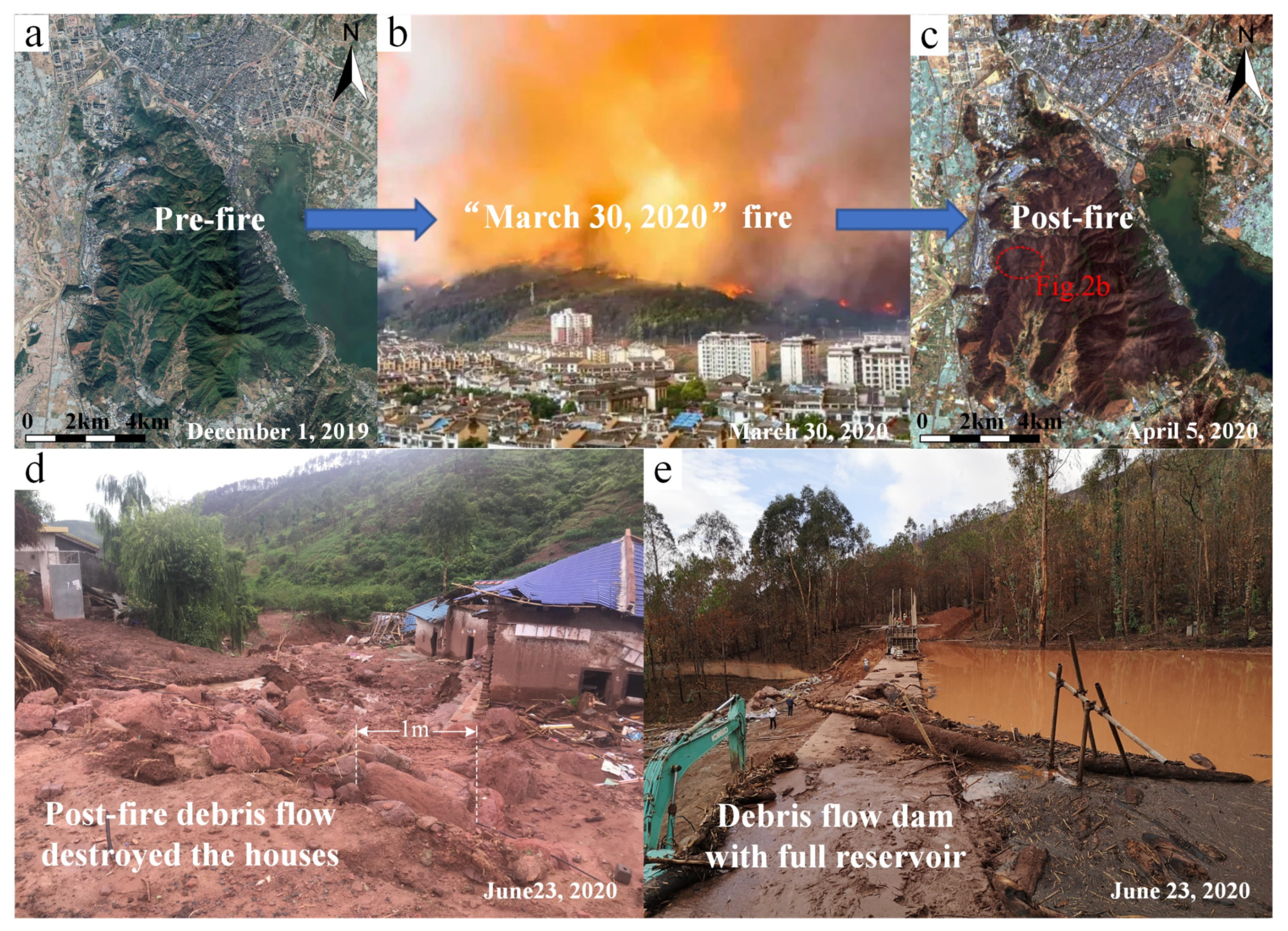
On 30 March 2020, a catastrophic wildfire occurred in the research area (Figure 2b). The wildfire lasted for three days, and the burned area was over 30 km2, accounting for approximately 75% of the total watershed area of Lushan Mountain, and 84.7% of the burned area was moderately or highly burned (Figure 2c). After the fire, the vegetation coverage of the burned area was reduced to about 15%, and the ground surface was exposed. A large amount of ash was accumulated on the hillslope surfaces (Figure 4a,b), and a large number of dead branches and trunks were scattered on the hillslope surfaces and in the main channel (Figure 4c). The possibility of PFDFs in the burned area is very high during rainstorms, which seriously threaten important facilities such as schools, gas stations, township government offices, and the Lushan–Qionghai scenic area near the foot of the hillslope. In addition, the fire killed 19 people and caused economic losses of approximately 100 million yuan.
In the first rainy season after the fire, the PFDF disasters did not cause casualties due to timely evacuations. However, in many watersheds, as shown in Figure 2d, houses and roads in the lower reaches were seriously damaged by the sudden debris flow due to a lack of treatment works. Most of the emergency prevention and control engineering facilities that were not completely developed were also buried or damaged by the debris flow (Figure 2e), resulting in total economic losses of approximately 140 million yuan.

3. Materials and Methods

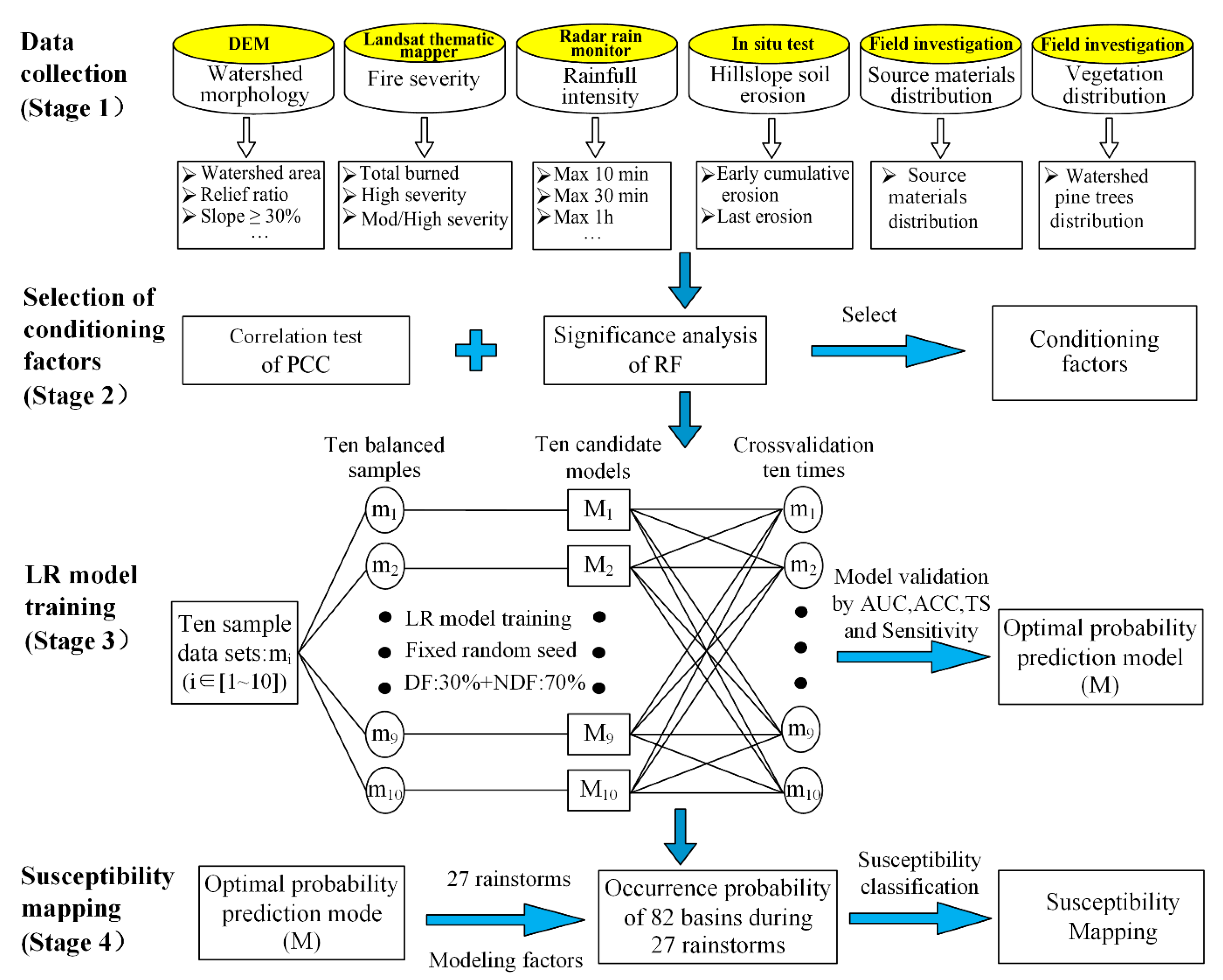
A flow chart of this study is shown in Figure 5; the study is divided into four steps: (1) Data preparation: compilation of PFDF inventory and conditional factors affecting PFDF initiation. (2) By performing Pearson correlation test and random forest (RF) significance analysis, the controlling factors of PFDF were extracted and the database was constructed. (3) The database was randomly and evenly divided into 10 balanced datasets of positive and negative samples. The LR model was used to train the model and the optimal model for predicting the probability of PFDF was obtained through 10 cross-validations. (4) The prediction model of the optimal PFDF probability was used to calculate the occurrence probability of PFDFs in different post-fire periods for each watershed in the study area. Susceptibility was graded according to different probability intervals. PFDF susceptibility maps were generated for different periods (1 May, 1 June, 1 July, 1 August, 1 September, and 1 October).

3.1. Database preparation

3.1.1. Post-Fire Debris Flow Inventory

Herein, using watersheds as assessment units, our field observations following each significant rainfall identified which watersheds produced debris flows or sediment-containing floods, based on the sedimentological and physical criteria described by Pierson [47]. The burned area was divided into 82 potential debris flow watersheds based on remote-sensing interpretations and field investigations conducted immediately after the fire (4 April 2020). A PFDF inventory was compiled based on the on-site investigation and aerial interpretation of the occurrence of debris flows during the 27 rainstorm events of the first rainy season after the fire (May–October 2020). Finally, we obtained 2214 hydrological response events, comprising 181 (~8.2%) debris flow events and 2033 non-debris flow events (all floods).

3.1.2. Post-Fire Debris Flow Conditioning Factors

No clear consensus is proposed on the PFDF-conditioning factors that should be involved in the modeling because the provenance initiation and movement mechanisms of PFDFs are extremely complex. According to previous studies and the data availability in the research site [7,17,21,42], 17 conditioning factors (including temporal and spatial factors) closely related to the formation process of PFDFs are selected, as shown in Table 1. Spatial factors include the following: six watershed morphological characteristic factors {watershed area (Area), relief ratio: the elevation change of the watershed divided by the length of the main ditch (RR), watershed average gradient (Gradient), proportion of watershed area with slope greater than or equal to 30% (Slope ≥ 30%), proportion of watershed area with slope greater than or equal to 50% (Slope ≥ 50%), and watershed shape factor: the ratio of the actual length of the watershed to the circumference of the same area circle of the watershed (WS)}; three characteristic factors of burning severity {proportion of moderately and severely burned area in the watershed (M/HS), proportion of the watershed burned at high severity (HS), and proportion of watershed area that has been burned (Total burned)}; four characteristic factors of rainfall intensity {maximum 10 min rainfall intensity (max 10 min), maximum 30 min rainfall intensity (max 30 min), maximum 1 h rainfall intensity (max 1 h), and maximum 24 h rainfall intensity (max 24 h)}; one vegetation-distribution characteristic factor (VD); and one source materials distribution characteristic factor (SMD). Temporal factors include the following two hillslope soil erosion factors {early cumulative erosion depth of the hillslope soil (ECE) and erosion depth of the hillslope soil during the last rainfall (LE)}. The method is as follows.
Watershed morphology characteristic factors: The steep topography directly affects the erosion rate of hillslopes and channels as well as the stability of sediments and leads to the surface runoff transited to a debris flow in the burned zone [8,48,49]. Based on the 12.5-m-resolution Digital Elevation Model (DEM), originated from the Alaska Satellite Facility (https://search.asf.alaska.edu/, accessed on 12 April 2020), ArcGIS spatial analysis tools were used to calculate the measured values of six watershed morphology factors as potential explanatory variables. These watershed morphological variables include the following: (1) area; (2) RR; (3) gradient; (4) slope ≥ 30%; (5) slope ≥ 50%; (6) WS.
Fire severity characteristic factors: The severity of wildfires is directly related to the reduction of soil protection layer and deterioration of physical soil properties. At the same time, it also increased the hillslope runoff response during rainfall and the hillslope susceptibility to erosion processes [16,50]. Simultaneously, high-intensity wildfires can significantly enhance the peak discharge in a post-fire watershed [16,51]. As shown in Figure 2a,c, the vegetation coverage decreased significantly after the fire. Using monitoring indicators such as the differentially normalized burning ratio (dNBR) constructed in the short-wave infrared (SWIR) and near-infrared (NIR) bands of multispectral remote sensing data, the burning severity of forest fires can be accurately calculated [52,53,54], which is a standard procedure for assessing spectral fire effects [55]. In this research, we obtained L1C-tiles of Sentinel-2 data before (26 March 2020) and after (6 April 2020) fire in the study area via the Earth Explorer (earthexplorer.usgs.gov, accessed on 12 April 2020) website. After atmospheric correction using a standalone version of the Sen2Cor-Processor (ESA) [56], the 8a-band (NIR) and 12-band (SWIR) were used to calculate dNBR by Equations (1) and (2) [55].
NBR = NIR SWIR NIR + SWIR
dNBR = NBR pre fire NBR post fire
Then, according to the fire intensity criterion proposed by Parsons, a field investigation was carried out and dNBR boundary values of different fire intensities were adjusted [26]. The fire severity in the watersheds was divided into four grades (Figure 6, Table 2): unburned, slight severity, moderate severity, and high severity [26,52,53,54]. Finally, using the ArcGIS spatial analysis tools, the three fire severity variables, M/HS, HS, and Total burned, were calculated for each watershed as potential explanatory variables which influence the initiation process of PFDF.
Rainfall intensity characteristic factors: PFDFs are usually triggered by short-term heavy rainfall [8,49,57,58]. Cannon et al. (2008) also pointed out that defining the rainfall thresholds for the rainfall intensity measured in a shorter duration (<20 h; Cannon et al., 2008) is necessary. Therefore, we selected four rainfall intensity variables having different durations (max 10 min, max 30 min, max 1 h, and max 24 h) as explanatory variables of rainfall conditions. These data derived from the radar rainfall monitor stations located within the 2-km radius of each watershed are interpolated using the ArcGIS10.5 software inverse distance weighting method to obtain rainfall data for each watershed in the study area [49,59].
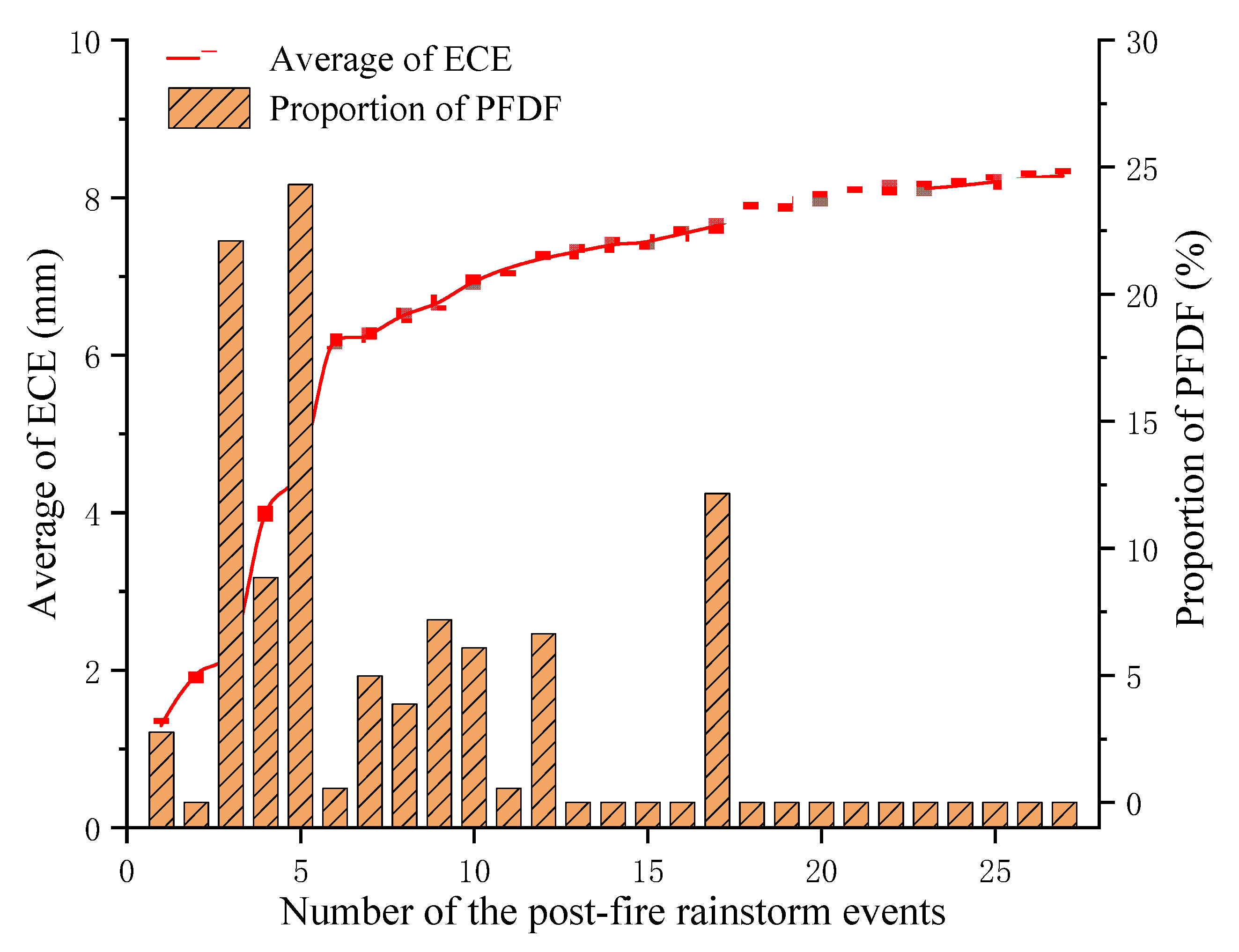
Hillslope soil erosion characteristic factors: After a wildfire, the rate of runoff and sediment transport on a hillslope will increase significantly compared with similar unburned areas [60,61]. The primary cause for this is that wildfires severely damage vegetation, causing the vegetation canopy, surface litter, and root layer to be partially or completely burned [62], and the high temperature of the burning causes the deterioration of soil properties making the surface soil of the hillslope loose, fragile, and easily eroded [54,63]. Generally, wildfires only affect soil to a depth of a few centimeters below the surface. Slope runoff scour and rill erosion after wildfires can thin or disappear fire-affected soil during heavy rains [64]. The resulting decrease in slope sediment availability may reduce the likelihood of debris flow [2,65,66]. Meanwhile, with the gradual restoration of vegetation after a fire, the properties of the hillslope surface soil will be improved and the soil permeability and erosion resistance will be enhanced. The hillslope runoff and erosion amount of the burned area will gradually decrease with time, thus reducing the susceptibility to PFDFs [2,25,28]. Figure 7 illustrates that the average of early cumulative erosion depth (ECE) increases while the PFDF occurrence frequency decreases with the increase of post-fire rainfall events (or time). Hence, ECE shows a negative correlation with PFDF susceptibility, which can be considered a temporal factor affecting the formation of PFDFs. We selected two hillslope soil erosion factors (ECE and LE) as potential explanatory variables that affect the initiation of PFDFs. The soil erosion factors of the hillslope are obtained from in situ tests. We first set the experimental plots in a hillslope of some watersheds in the study area, where the geological environmental conditions were similar, and the slope surface was relatively undamaged; set up erosion monitoring plots in areas with various fire severity, hillslope gradient, and hillslope length; and placed a total of 1600 erosion pins. Then, we measured the hillslope erosion depth after each rainstorm and obtained a total of twelve sets of data through continuous in situ tests during the entire rainy season (May to October 2020). Using a nonlinear fitting method, the computing model of hillslope erosion on different fire severities of the burned area is obtained (Equation (3)), which quantitatively describes the hillslope soil erosion depth in different watersheds of the research area. Finally, the spatial analysis tool in the ArcGIS platform is conducted to calculate the ECE and LE of each watershed.
D = 0.1753 · E X P dNBR · ln R · S 0.2176 · L 0.1302
n = 985 ,   R 2 = 0.6558 , P < 0.001
where D is the hillslope erosion depth (mm), R refers to the accumulated rainfall erosivity (MJ · mm/(ha · h)), S is the slope gradient (°) and L is the slope length (m) (Note: The derivation Equation (3) was presented in the paper titled: “Characteristics and calculation of the dynamic reserves of hillslope erosion materials in burned areas in Xichang, China, on 30 March 2020”, which is currently under minor revision at Catena).
Source materials distribution characteristic factors: Loose solid materials are one of the three basic preconditions for the development of debris flow. Abundant surface ash and a loose sand layer formed on the hillslope after the wildfire destroyed the tree canopy and surface deciduous layer (Figure 4a,b). The soil structure of the hillslope is disturbed by high-temperature baking. During a rainstorm, the ash and loose sediment on the hillslope will be easily initiated to cause a PFDF. Simultaneously, the ash flow increases the bulk density of the mud and rock fluid, which in turn increases its ability to carry larger rocks [67]. The dynamic material sources distributed near the gully, such as loose sediment, ash, fragments of gravel, dead branches and trunks, and other loose materials (Figure 4b–d), are easy to initiate under the influence of an ash flow, which will increase the erosive capacity of the debris flow and easily block the gully, resulting in the amplification effect of debris flow blocking. Therefore, through a 20-day field measurement (GPS fixed point measurement) on the burned area immediately after the fire, the Dynamic material source distribution in each watershed was recorded and the specific value between the supply length of the sediment along the main channel and the main channel length in the watershed was selected as the potential explanatory variable for the initiation of PFDF, which is a variable that can be divided into four types according to the Investigation Standard of Specification of Geological Investigation for Debris Flow Stabilization [68]. Categories 1–4 characterize this variable as <10%, 10–30%, 30–60%, and >60%, respectively [21].
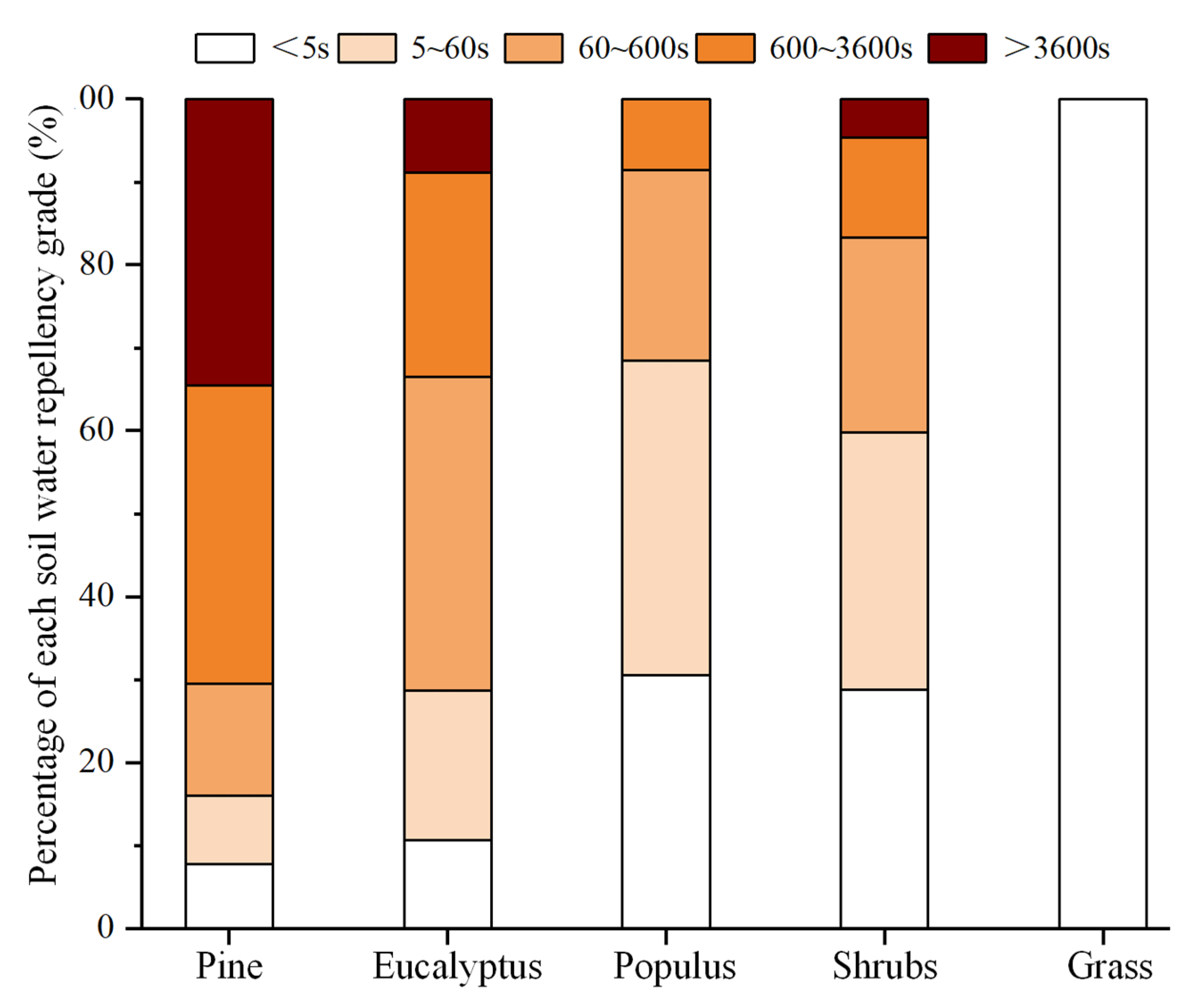
Vegetation distribution characteristic factors: Wildfire induces the manufacture or improvement of soil water repellency. It decreases the soil permeability and enhances the hillslope runoff, thus, aggrandizing the susceptibility to PFDFs [31,32]. The water repellency of soil in a pine forest increases considerably after wildfires compared with other forest vegetation [69]. During the field survey of the burned area, we tested the water repellency of soil through Water Drop Penetration Time (WDPT) and found that soil water repellency of pine forest fire areas significantly increased (most are severe to extreme in water repellency) [70]. For other vegetation types, such as eucalyptus, populus, and shrubs, the soil water repellency is mostly light to severe whereas the soil under grass has no water repellency (Figure 8). Concurrently, the content of pine oil is higher and the branches are flammable and burn more violently, resulting in more serious burns to the soil structure and vegetation roots and increasing the soil’s erodibility [54]. Hence, through aerial image interpretations and field investigations, combined with data provided by the local forestry department, the species and vegetation distribution in each watershed were obtained and the percentage of the primordial pine covered area (before the fire) in the watershed was selected as the potential explanatory variable for the initiation of PFDF, which was allocated into five categories and the categories 1–5 represent the variable in the watershed as <20%, 20–40%, 40–60%, 60–80%, and 80–100%, respectively [21].

3.2. Selecting the Post-Fire Debris Flow Conditioning Factors

Owing to the fact that redundant information may generate noise in modeling and reduce the prediction ability, selecting appropriate conditioning factors for PFDF susceptibility modeling is vital. Therefore, the Pearson correlation coefficient (PCC) and the RF method were employed to select the PFDF conditioning factors herein.
PCC is usually used to measure the linear correlation of two variables as an efficient method. Its value ranges from −1 to 1, and the absolute value will exceed 0.5 if the two variables have a strong correlation. The RF algorithm developed by Breiman (2001) is a nonparametric statistical technique utilized for regression and classification and has been widely used in the modeling of debris flows, landslides, and other disasters [9,21,71,72]. Furthermore, the RF model can play an important role in ranking the importance of variables and measuring the importance of selected conditioning factors by obtaining the Gini coefficient [73]. This study is based on the Scikit-Learn library in the Python3.6.5 environment for RF modeling. The main model parameters “n_estimators”, “max_features” and “max_depth” were set as “500”, “17” and “10”, respectively. Besides, the output value of “feature_importances” showed the importance of each conditioning factor [21,72].
Therefore, we first modeled all sample data (2214) and calculated the “feature_importances” (importance or contribution) of each PFDF conditioning factor based on the RF model (repeating 10 times and taking the average). Then PCC was utilized to precisely describe the correlation of all the conditioning factors. If one of them shows a strong correlation with other factors (absolute value >0.5), it will be regarded as an unnecessary redundant factor. If two or more two factors show a significant correlation, only the factors with higher importance could remain. Finally, the LR model was established according to the remaining conditioning factors.

3.3. Model

The LR algorithm is a classical machine learning algorithm, which is usually used for modeling the statistical likelihood of a binary response variable. Especially, it has been widely used to predict the occurrence possibility of PFDFs in the Western United States [7,8,38,44,45,74,75]. The LR approach is advantageous because it is computationally simple and can provide the statistical possibility for the occurrence of debris flows for different magnitudes of a storm in a geospatial format at the scale of a stream segment or watershed [8]. In addition, the predictive model can be presented more intuitively compared with other machine learning methods, which is convenient for engineering applications. The probability of occurrence (P) of PFDFs according to LR is given as
P = e x 1 + e x ,
where P is a number ranging from 0 to 1, representing the statistical possibility of the occurrence of PFDFs (where values approaching 1 indicate an increasing possibility) and x is determined by the link function:
x = β + C 1 X 1 + C 2 X 2 + + C n X n ,
where β and C1, C2, …, Cn are empirically derived parameters and X1, X2, …, Xn represent independent explanatory variables that impact the occurrence of the PFDF event.

3.4. Model Training and Validation

Herein, the LR model is used to model the susceptibility to PFDF. First, 2033 monitored non-debris flow events were evenly and randomly divided into 10 negative samples, which were combined with 181 debris flow events to form 10 sample datasets. The 70% data of each dataset were divided into the training samples, and the remaining 30% data were divided into validation samples. The unbalanced binary results were interpreted using stratified random sampling [76]. Then, the LR model was adopted (different random seed numbers were selected) to conduct the same modeling training for 10 sample datasets in the following two steps: (1) Through 100 iterations of model training (10 sample datasets × 10 times of random training), the training model Mij that simultaneously reaches the maximum values of TS, Sensitivity, AUC, and Accuracy in each sample dataset is screened and named as candidate model Mi (where i represents the ith sample data set, j represents the number of random seeds of the jth LR model, and i and j are integers ranging from 1 to 10). (2) Each candidate model Mi is cross validated in turns with 10 sample datasets 10 times, and an optimal candidate model which has the maximum magnitude of average values of the model evaluation indexes TS, Sensitivity, AUC, and Accuracy is selected, that is, the final prediction model M. Finally, the map of PFDF susceptibility is generated. The Python language with a 3.6.5 environment was used for developing the predicted model and preprocessing geospatial data.
To evaluate the model performance, the contingency table (Table 3) was employed to measure the number of correct and false events in the predicted outcomes. True positive (TP) is the sum of the outcomes that correctly predict debris flow events, and true negative (TN) is the number of the non-debris flow events correctly predicted. False positive (FP) represents the falsely predicted number of all debris flow events, and false negative (FN) indicates the number of the non-debris flow events which were wrongly predicted in debris flow. According to Table 3, the metrics, such as accuracy, sensitivity, TS, and AUC were calculated herein to evaluate the predictive performance of the model. Those indexes were widely used to evaluate and validate the PFDF prediction models in the previous study and can be obtained from the following equations [8,10,42].
A c c u r a c y = T P + T N T P + F P + T N + T P
S e n s i t i v i t y = T P T P + F N
T S = T P T P + F N + F P
Among them, accuracy (ACC) represents the number of samples with correct classification/the number of all samples; sensitivity (also known as true positive rate) corresponds to the number of positive samples predicted to be positive/the actual number of positive samples. TS (critical success index) represents a measure of the overall performance of the classifier model where a perfect model score would equal one, and each incorrect prediction (FP or FN) will reduce the value of TS [77]. The area under the curve (AUC) value is the common index to evaluate the overall performance of the prediction model, which can be classed as follows: poor (50–60%), moderated (60–70%), good (70–80%), very good (80–90%), and excellent (90–100%) [8,10,42,72].

4. Results

4.1. Modeling Factor Selection

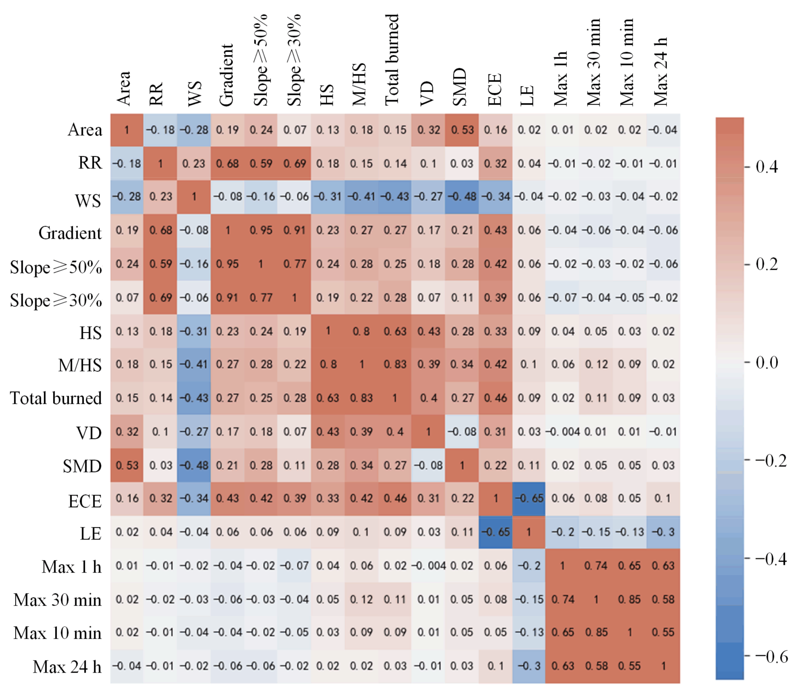
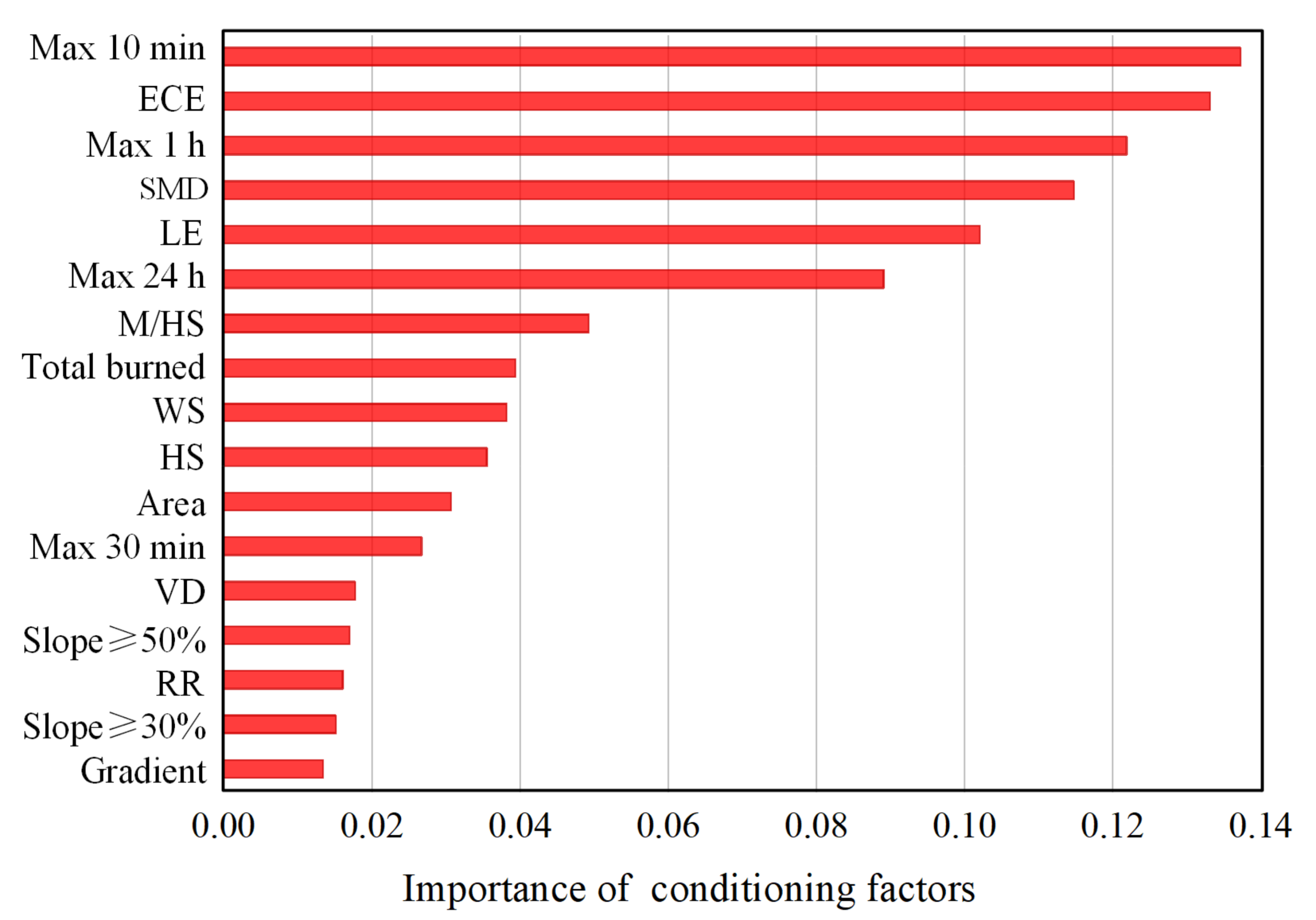
Figure 9 illustrates the correlation coefficients among the 17 initial conditioning factors, and Figure 10 illustrates the importance (or contribution) ranking of each conditioning factor using the RF method (the average of 10 calculations). Based on the results obtained from importance analysis, max 10 min is the primary conditioning factor (0.1375) impacting the prediction the occurrence of PFDFs, followed by ECE (0.1334), max 1 h (0.1221), SMD (0.1150), LE (0.1022), max 24 h (0.0893), M/HS (0.0494), total burned (0.0395), WS (0.0383), HS (%) (0.0357), area (0.0308), max 30 min (0.0268), VD (0.0179), slope ≥ 50% (0.0171), RR (0.0162), slope ≥ 30% (0.0152), and gradient (0.0135). Therefore, in addition to the rainfall factors, ECE, SMD, LE, and M/HS are the main controlling factors affecting the formation of PFDFs.
According to the results of correlation analysis, there are three groups of multiple factors in the initial conditioning factors that are strongly correlated with each other. These groups include four watershed morphology factors (RR, gradient, slope ≥ 50%, and slope ≥ 30%), three fire severity factors (HS, M/HS, and total burned), and four rainfall intensity factors (max 10 min, max 30 min, max 1 h, and max 24 h). Based on the importance of the conditioning factors (Figure 10), we only retained the conditioning factor that contributed the most to the prediction of the PFDF among the three groups of conditioning factors: slope ≥ 50%, M/HS, and max 10 min. Furthermore, the correlations between area and SMD and between ECE and LE are extremely significant. Similarly, we retained SMD and ECE, which have a greater contribution to the prediction of PFDF. The remaining factors, WS and VD, are not significantly related to any other factors; thus, they were also retained. The seven remaining conditioning factors are the final PFDF susceptibility modeling factors: max 10 min, ECE, M/HS, SMD, WS, VD, and slope ≥ 50%.

4.2. Optimal Probability Prediction Model Selection

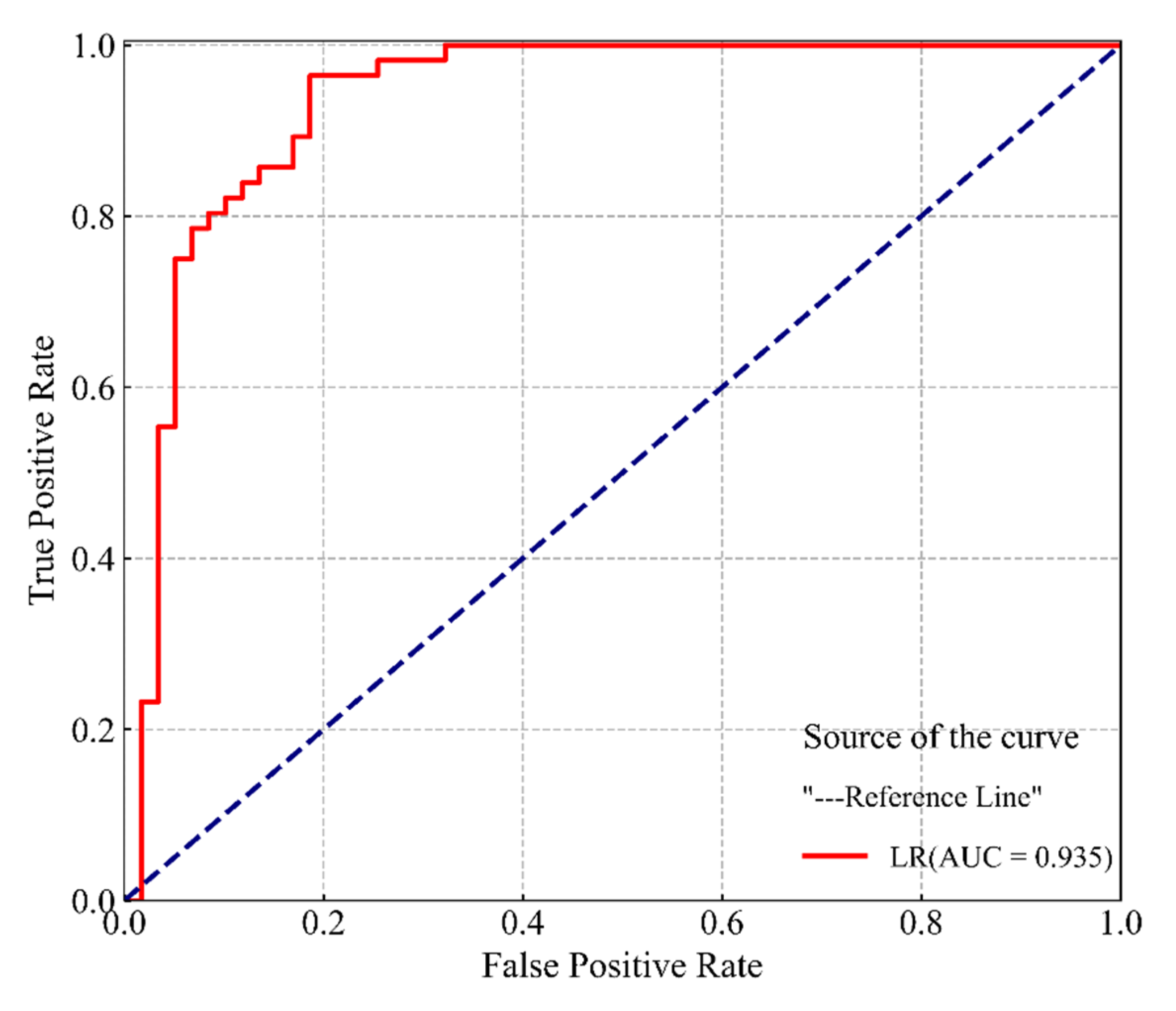
To obtain the optimal training model for the prediction of PFDF susceptibility, we fixed the number of random seeds to perform the same modeling training on 10 sample datasets. First, 10 candidate models Mi were selected through 100 repetitions of model training (10 sample datasets × 10 times of random training). Then, each candidate model was cross-validated with 10 sample datasets, 10 times each. The cross-validation results are shown in Figure 11, which shows that the 10 candidate models all show good predictive performance, indicated by the AUC and ACC that are greater than 0.915 and 0.83, respectively. M1 performed the best, with average values of AUC, sensitivity, ACC, and TS in the cross-validation results being 0.924, 0.89, 0.859, and 0.749, respectively, which were the maximum values among the 10 candidate models. Therefore, M1 is determined as the final PFDF probability prediction model (Equation (9)), and the verification results of the prediction performance of M1 are shown in Figure 12 and Table 4. The results show that the M1 exhibits a good predictive performance for which the AUC is 0.935, the sensitivity is 0.964, the accuracy is 0.887, and the TS is 0.806.
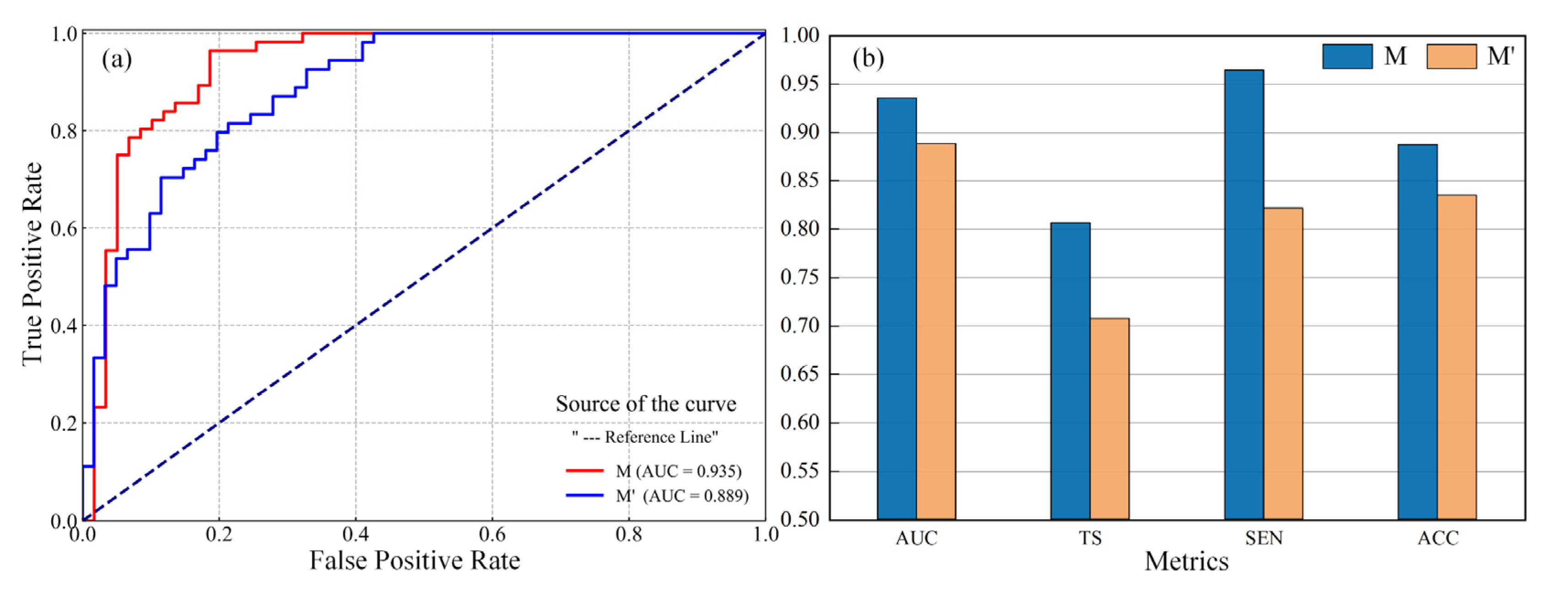
In order to verify the advantages of the modeling method in this study, we compared the prediction effects of the spatiotemporal prediction model (the optimal prediction model of this study, named M) with a spatial prediction model (the modeling factors do not include ECE; however, the model uses the same training, named M′) during the modeling process. We also directly conducted model training on unbalanced samples (total sample dataset) and verified the training with the total sample dataset. The results show that the prediction performance of the spatial prediction model without considering the temporal factor is significantly lower than that of the spatiotemporal prediction model, in which Sensitivity, AUC, TS, and ACC are decreased by 14.3%, 1.4%, 10%, and 5.2%, respectively (Figure 13). Compared with the balanced sample modeling, the accuracy of the unbalanced sample model is increased by 8.7%; however, its sensitivity, TS, and AUC are lowered by 61.9%, 8.9%, and 1.5%, respectively (Table 5). This implies that the model built with unbalanced samples not only reduces the overall prediction performance of the prediction model but also greatly increases the false-negative rate of debris flows. Rather than reducing the false positive rate, it is more practical to avoid the increase of the false-negative rate.
P = e 0.393 1.314 X 1 + 2.357 X 2 + 2.744 X 3 + 0.448 X 4 + 0.182 X 5 0.51 X 6 + 0.035 X 7 1 + e 0.393 1.314 X 1 + 2.357 X 2 + 2.744 X 3 + 0.448 X 4 + 0.182 X 5 0.51 X 6 + 0.035 X 7 ,
where P represents the occurrence probability of a PFDF; X1 is the watershed shape coefficient (WS); X2 is the proportion of burn watershed area with slope ≥ 50% (slope ≥ 50%); X3 is the proportion of the watershed area burned at moderate and high severity (M/HS); X4 is the ratio of the supply length of the sediment along the main channel in the watershed (SMD); X5 is the original pine tree coverage area in the watershed (VD); X6 is the cumulative erosion depth of the hillslope soil before the PFDF occurs (ECE (mm)); X7 is the maximum 10 min rainfall intensity (max 10 min (mm/h)).

4.3. Susceptibility Mapping

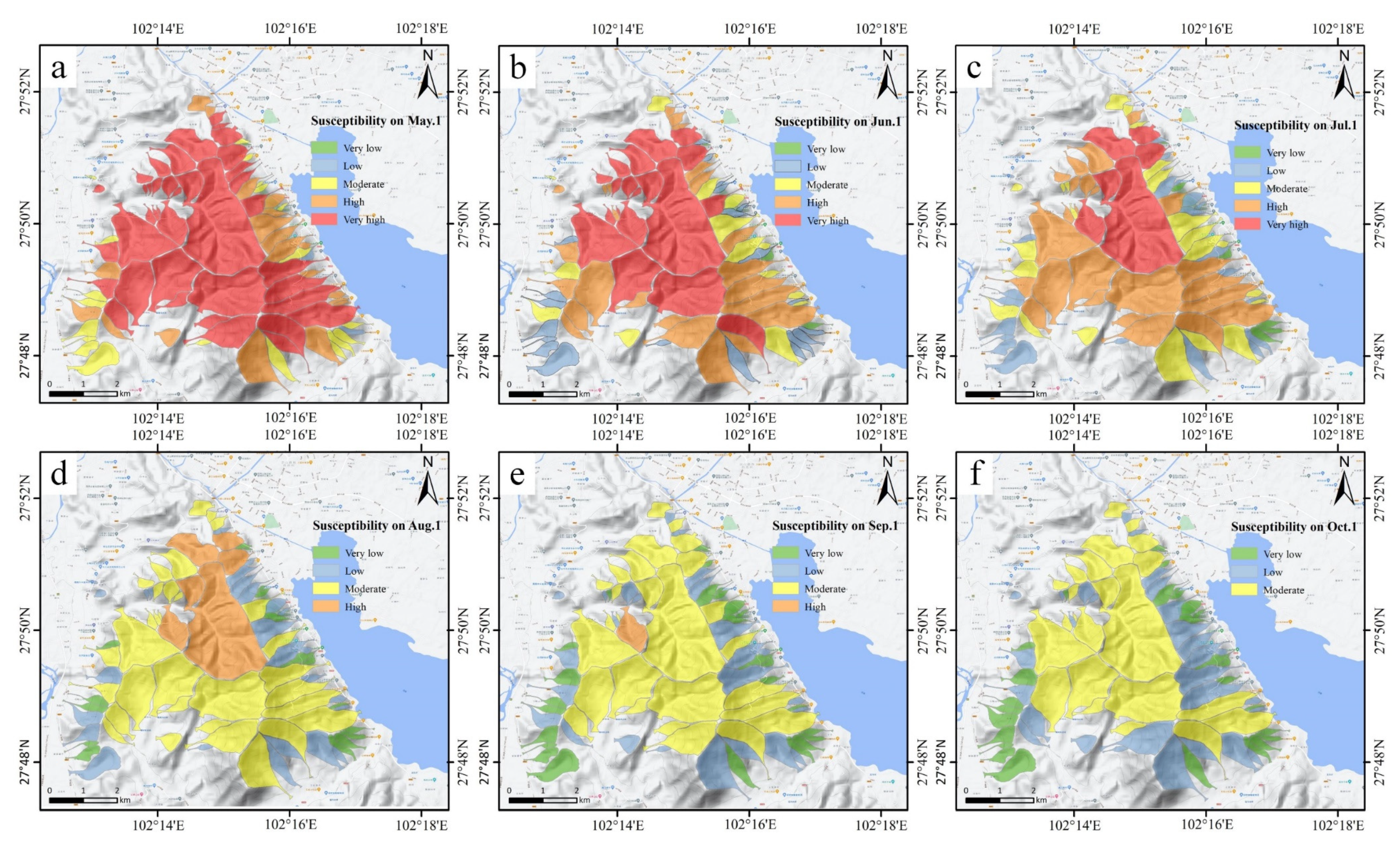
To explore the evolution behaviors of PFDF susceptibility over time and space, this study is based on the optimal prediction model (M1) of the occurrence probability for PFDF, and all PFDF conditioning factors (rainfall intensity set as the average value of max 10 min in 27 rainstorm events) are substituted into M1 during the 27 rainstorm events after the fire. The occurrence probability (P) of PFDF in each watershed is calculated for different post-fire periods. Then, P is equally divided into five levels corresponding to susceptibility to PFDF: very low (0–0.2), low (0.2–0.4), moderate (0.4–0.6), high (0.6–0.8), and very high (0.8–1.0). Finally, ArcGIS is used to map the susceptibility to PFDF in 82 watersheds in the research area at different post-fire periods (1 May, 1 June, 1 July, 1 August, 1 September, and 1 October; see Figure 14 and Table 6). Figure 15 shows the behavior of the percentages of each PFDF susceptibility level over time. As is shown in Figure 14 and Figure 15, the susceptibility to PFDF decreases with the increase of the number of post-fire rainfall events (i.e., the increase of time). At the beginning of the rainy season (Figure 14a), among the 82 potential PFDF watersheds in the study area, the numbers of very low, low, moderate, high, and very high susceptibility watersheds were 1, 3, 20, 19, and 39, respectively, accounting for 1.2%, 3.7%, 24.4%, 23.2%, and 47.6%, respectively. At the end of the rainy season (Figure 14f), the proportion of very high and high susceptibility watersheds decreased to 0 whereas the proportion of very low, low, and moderate susceptibility watersheds increased to 35.4%, 35.6%, and 28.1%, respectively. May–July (about the first six rainstorm events after the fire) was a period of significant attenuation of PFDF susceptibility in each watershed (Figure 14a–c), almost all watersheds moved to a lower susceptibility level (except those that were already very low). By 1 August, the very high susceptibility watersheds had completely disappeared (Figure 14d) and most of the high susceptibility watersheds had turned into low to moderate susceptibility. As of 1 October, all the high and very high susceptibility watersheds have been transformed into very low to moderate susceptibility watersheds (Figure 14f).

4.4. Validation of Susceptibility Evaluation Results

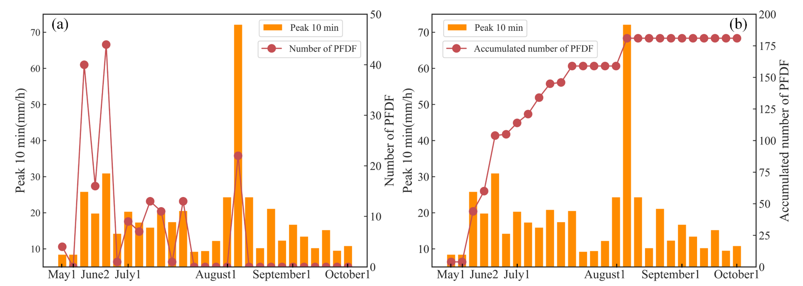
Figure 3 and Figure 16 show the in-site investigation of the PFDF occurrence regularity in the first rainy season following the fire. As shown in Figure 3 and Figure 16, May–July is the peak rainfall stage of the rainy season, and it is also the high susceptibility period for PFDFs. Approximately 50% of the watershed has high or very high susceptibility (Figure 15). Therefore, the rainfall threshold for PFDF in this stage is not high (the average max 10 min rainfall intensity reaches 19.3 mm/h, and the lowest max 10 min rainfall intensity is about 8.4 mm/h), and the incidence of PFDFs is as high as 85.6% of all PFDFs in the entire rainy season. Although August is still the peak rainfall stage of the rainy season, the early rainstorms not only mobilized a large number of material sources on the hillslope but also moisturized the soil and enabled the vegetation to quickly recover. This will significantly increase the permeability and erosion resistance of the hillslope soil and greatly weaken the susceptibility to PFDFs. As shown in Figure 14 and Figure 15, the watersheds with very high susceptibility to PFDFs had completely disappeared by 1 August (Figure 14d) and most of the high susceptibility watersheds had become low to moderate susceptibility. Therefore, the occurrences of PFDFs in August only accounted for 14.4% of the total occurrences and the rainfall threshold (max 10 min) was as high as 72 mm/h. From September to October, almost all of the high and very high susceptibility watersheds were transformed into very low to moderate susceptibility watersheds and approximately 72% of the watersheds were very low to low susceptibility watersheds (Figure 14e, f). Therefore, there were no PFDFs even when the max 10 min rainfall intensity reached 24.4 mm/h at this stage. In summary, the temporal evolution of PFDF susceptibility in different watersheds presented by the prediction model is basically consistent with the development behavior of on-site PFDFs.

5. Discussion

In this paper, based on the logistic regression (LR) model, a quantitative prediction model of PFDF susceptibility in each watershed at different post-fire periods was established. It gives insight into the evolution law of PFDF susceptibility after wildfire and further improves our ability to predict and mitigate PFDF disasters according to the following aspects: (1) We analyzed all the modeling variables and found the most influential variables. (2) The modeling variables of the prediction model include one temporal factor and six spatial factors, which endow the model with spatio-temporal prediction ability; (3) The prediction accuracy of the model is improved by using balanced positive and negative sample data.
The difference between our study and previous similar studies is how to introduce the temporal factors (ECE) into the traditional susceptibility mapping method. This study used the in-situ tests during the entire rainy season (May to October 2020) to obtain the data containing a total of 1600 erosion pins. Based on these data, we obtained the average of early cumulative erosion depth (ECE) in the different post-fire periods. The ECE is defined as Equation (3), which is associated with the cumulative rainfall, fire intensity, hillslope gradient, and hillslope length. The different period of ECE after the fire is shown in Figure 7. Compared with other temporal factors (e.g., hillslope surface vegetation recovery rate, soil water repellency and permeability) [29,36,78,79], ECE data is easier to obtain, quantify, and apply to other burned watersheds. As the integrated factor, ECE can directly reflect the response of runoff to changes in hillslope soil characteristics and the availability of hillslope sediment [2,65]. According to the above advantage, this study selected the ECE as the temporal factor to reflect the tendency of PFDF susceptibility over time, which is generally ignored in the previous models [6,7,8,10]. The importance analysis based on the RF model shows that the ECE is the most important factor except the rainfall (Figure 10). In addition, the ECE factors can effectively improve the predictive model performance, as shown in Figure 13. Compared to the M′ model, the sensitivity, AUC, TS, and ACC of the M model increase 14.3%, 1.4%, 10%, and 5.2%, respectively.
The study area is located at the junction of town and forest and has been seriously threatened by the PFDF after the fire. In a traditional prevention strategy, the high-risk area can be identified but the duration of the threat of PFDF is unclear. During the whole rainy season after the fire, as soon as it rained, downstream communities were forced to evacuate. The proposed model by this study can help decision-makers to plan specific and improved prevention strategies in different post-fire periods.
A review of discharge-based recovery times following wildfire found a typical range of two to seven years for watershed hydrologic recovery [29]. However, the hydrological recovery of the watershed in the study area is very rapid. From Figure 14 and Figure 15, it can be seen that the PFDF in the study area has a short duration, about 85.6% of the debris flow occurred in the first three months after the fire (in the first six rainfall events). About 4.5 months after the fire, the ECE value of the watershed became basically stable (Figure 7). After that and until the end of the second rainy season, the recorded hydrologic response events in the study area are dominated by floods. This study suggested that human activities play an important role in the recovery of watersheds after the fire, which caused this phenomenon [29]. For example, the drone seeding of grass seeds and artificial planting of trees accelerated the natural recovery of vegetation and soil, which significantly reduced the duration of PFDF disasters in the study area. In addition, suitable climatic environments, such as moderate altitude, sufficient sunshine, and rain, moderate rainfall in the first month of the rainy season also accelerated the natural recovery of vegetation and soil properties after a fire.
According to statistics, the majority of PFDFs are initiated by hillslope runoff [38], almost 85% of PFDFs occurred within the first 12 months following a wildfire, and 71% occurred within the first six months [80]. In general, the recovery of vegetation and soil in the watershed may need two years or more. Although the data used by this study only contains seven months, the proposed model also has the potential to predict more than one rainy season after fires. In the follow-up study, we will continue to monitor the temporal evolution of hillslope erosion in burned areas and add new experimental sample plots to obtain more test data for the medium- to long-term prediction model development. Lithology, soil thickness, and other factors were not taken into account due to the limitations of data availability, which will consider in the following study.
To ensure the prediction accuracy of the model, the high spatial resolution of DEM and remote sensing images should be used to calculate the topographic data (Slope ≥ 50% and WS) and the fire severity data (M/HS). The accuracy of rainfall intensity (max 10 min) depends on the rainfall monitoring equipment. It is better to collect rainfall data per minute and set the rainfall monitoring station within 1 km from the watershed. VD and SMD should be acquired through on-site investigation and classified and quantified, so there may be certain challenges and subjective errors in the data acquisition process. In future research, the higher resolution remote sensing image will be used to eliminate the error of data acquisition. In addition to the fitting function (Equation (3)), the acquisition of ECE can also be used to monitor the average cumulative erosion of hillslope soil via high-resolution change detection technologies [81]. To sum up, most of the modeling variables of the prediction model in this study are composed of publicly available geospatial data and rainfall data. The method proposed in this study can be applied to the development of spatio-temporal prediction models for the susceptibility of post-fire debris flows in other regions.

6. Conclusions

In this paper, 82 watershed areas burned by the “30 March 2020” fire in Xichang City, Sichuan Province are selected as an illustrative example. Seven conditioning factors consist of temporal factors and spatial factors are extracted by the remote sensing interpretation, field investigations, and situ test, after correlation and importance analysis. The logistic regression (LR) is adopted to establish prediction models through 10 cross-validations. The main conclusions are as follows:
(1)
Max 10 min is the primary factor impacting the initiation of post-fire debris flow (weight: 0.1375), ECE (0.1334), SMD (0.1150), and M/HS (0.0494) are the primary controlling factors affecting the initiation of post-fire debris flow except for rainfall.
(2)
The validation results show that the LR has good prediction performance, in which the AUC is 0.935, the Sensitivity is 0.964, the Accuracy is 0.887, and the TS is 0.806.
(3)
The susceptibility of PFDF has significantly reduced over time. After two months of wildfire, the proportions of very low, low, moderate, high, and very high susceptibility are 1.2%, 3.7%, 24.4%, 23.2%, and 47.6%, respectively. After seven months of wildfire, the proportions of high and very high susceptibility decreased to 0, while the proportions of very low to medium susceptibility increased to 35.4%, 35.6%, and 28.1%, respectively.
(4)
Human activity plays an important role in the recovery of watersheds after the wildfire. The drone seeding of grass seeds and artificial planting of trees accelerated the natural recovery of vegetation and soil, which significantly reduced the duration of PFDF disasters in the study area.
This study can give insight into the evolution mechanism of PFDF over time and reflect the important influence of human activity after the wildfire. Although the study focuses on the specific area, the method proposed by this study can guide the planning of mitigating the PFDF risk on the other burned area.

Author Contributions

Conceptualization, T.J. and C.X.; methodology, X.H. and B.L.; software, C.X. and T.J.; validation, T.J. and K.H.; investigation, T.J., C.X., Y.Y. and Y.W.; resources, X.H.; data curation, T.J. and C.X.; writing—original draft preparation, T.J. and C.X.; writing—review and editing, B.L., G.M., G.L., K.H. and X.C.; supervision, X.H. and M.H.; project administration, X.H.; funding acquisition, X.H. All authors have read and agreed to the published version of the manuscript.

Funding

We gratefully acknowledge the financial support of the National Natural Science Foundation of China (Grant No. 41731285).

Data Availability Statement

This paper has uploaded the code of LR modeling, and PFDF conditional factor importance analysis based on the RF model. Please refer to https://github.com/JinduoduoGitHub/LR-model (accessed on 1 March 2022).

Acknowledgments

We are grateful to Engineers Wanqing Yin of Xichang Natural Resources Bureau and Engineer Zhubei Huo of Southwest Nuclear Industry 281 Geological Team for their help in field investigations. We are also grateful to the reviewers of this manuscript for their good suggestions and useful comments.

Conflicts of Interest

The authors declare that they have no known conflict interests or personal relationships that could have appeared to influence the work reported in this paper.

References

  1. Wall, S.A.; Roering, J.J.; Rengers, F.K. Runoff-initiated post-fire debris flow Western Cascades, Oregon. Landslides 2020, 17, 1649–1661. [Google Scholar] [CrossRef]
  2. Thomas, M.A.; Rengers, F.K.; Kean, J.W.; Mcguire, L.A.; Ebel, B.A. Postwildfire soil-hydraulic recovery and the persistence of debris flow hazards. J. Geophys. Res. Earth Surf. 2021, 126, e2021JF006091. [Google Scholar] [CrossRef]
  3. Lancaster, J.T.; Swanson, B.J.; Lukashov, S.G.; Oakley, N.S.; Lee, J.B.; Spangler, E.R. Observations and analyses of the 9 January 2018 debris-flow disaster, Santa Barbara County, California. Environ. Eng. Geosci. 2021, 27, 3–27. [Google Scholar] [CrossRef]
  4. Shakesby, R.A.; Doerr, S.H. Wildfire as a hydrological and geomorphological agent. Earth-Sci. Rev. 2006, 74, 269–307. [Google Scholar] [CrossRef]
  5. Diakakis, M. Flood seasonality in Greece and its comparison to seasonal distribution of flooding in selected areas across southern Europe. J. Flood Risk Manag. 2017, 10, 30–41. [Google Scholar] [CrossRef]
  6. Addison, P.; Oommen, T. Post-fire debris flow modeling analyses: Case study of the post-Thomas Fire event in California. Nat. Hazards 2020, 100, 329–343. [Google Scholar] [CrossRef] [Green Version]
  7. Cannon, S.H.; Gartner, J.E.; Rupert, M.G.; Michael, J.A.; Rea, A.H.; Parrett, C. Predicting the probability and volume of postwildfire debris flows in the intermountain western United States. Geol. Soc. Am. Bull. 2010, 122, 127–144. [Google Scholar] [CrossRef]
  8. Staley, D.M.; Negri, J.A.; Kean, J.W.; Laber, J.L.; Tillery, A.C.; Youberg, A.M. Prediction of spatially explicit rainfall intensity–duration thresholds for post-fire debris-flow generation in the western United States. Geomorphology 2017, 278, 149–162. [Google Scholar] [CrossRef]
  9. Napoli, M.D.; Marsiglia, P.; Martire, D.D.; Ramondini, M.; Calcaterra, D. Landslide susceptibility assessment of wildfire burnt areas through earth-observation techniques and a machine learning-based approach. Remote Sens. 2020, 12, 2505. [Google Scholar] [CrossRef]
  10. Nikolopoulos, E.I.; Destro, E.; Bhuiyan, M.A.E.; Borga, M.; Anagnostou, E.N. Evaluation of predictive models for post-fire debris flows occurrence in the western United States. Nat. Hazards Earth Syst. Sci. Discuss. 2018, 18, 2331–2343. [Google Scholar] [CrossRef] [Green Version]
  11. Cannon, S.H.; Powers, P.S.; Savage, W.Z. Fire-related hyperconcentrated and debris flows on Storm King Mountain, Glenwood Springs, Colorado, USA. Environ. Geol. 1998, 35, 210–218. [Google Scholar] [CrossRef]
  12. Hu, X.W.; Wang, Y.; Yang, Y. Research actuality and evolution mechanism of post-fire debris flow. J. Eng. Geol. 2018, 26, 1562–1573. [Google Scholar]
  13. Cannon, S.H. Debris-flow generation from recently burned watersheds. Environ. Eng. Geosci. 2001, 7, 321–341. [Google Scholar] [CrossRef]
  14. Gartner, J.E.; Cannon, S.H.; Bigio, E.R.; Davis, N.K.; Parrett, C.; Pierce, K.L.; Rupert, M.G.; Thurston, B.L.; Trebish, M.J.; Garcia, S.P. Compilation of data relating to the erosive respose of 606 recently-burned basins in the Western United States. US Geol. Surv. Open-File Rep. 2005, 1218. Available online: https://pubs.usgs.gov/of/2005/1218/ (accessed on 1 March 2022).
  15. Nyman, P.; Sheridan, G.J.; Smith, H.G.; Lane, P. Evidence of debris flow occurrence after wildfire in upland catchments of south-east Australia. Geomorphology 2011, 125, 383–401. [Google Scholar] [CrossRef]
  16. Nyman, P.; Smith, H.G.; Sherwin, C.B.; Langhans, C.; Lane, P.; Sheridan, G.J. Predicting sediment delivery from debris flows after wildfire. Geomorphology 2015, 250, 173–186. [Google Scholar] [CrossRef]
  17. Hu, X.W.; Jin, T.; Yin, W.Q.; Huo, Z.B.; Song, Y.P.; Zhang, S.K.; Wang, Y.; Yang, Y. The characteristics of forest fire burned area and susceptibility assessment of post-fire debris flow in Jingjiu Township, Xichang City. J. Eng. Geol. 2020, 28, 762–771, (In Chinese with English abstract). [Google Scholar]
  18. Flannigan, M.D.; Krawchuk, M.A.; De Groot, W.J.; Wotton, B.M.; Gowman, L.M. Implications of changing climate for global wildland fire. Int. J. Wildland Fire 2009, 18, 483–507. [Google Scholar] [CrossRef]
  19. Westerling, A.L.; Hidalgo, H.G.; Cayan, D.R.; Swetnam, T.W. Warming and earlier spring increase western US forest wildfire activity. Science 2006, 313, 940–943. [Google Scholar] [CrossRef] [Green Version]
  20. Oakley, N.S. A Warming Climate Adds Complexity to Post-Fire Hydrologic Hazard Planning. Earth’s Future 2021, 9, e2021EF002149. [Google Scholar] [CrossRef]
  21. Jin, T.; Hu, X.W.; Xi, C.J.; He, K.; Yang, Y.; Cao, X.C. Susceptibility assessment of “2020.3.30” Xichang post-fire debris flow using a machine learning method. IOP Conf. Ser. Earth Environ. Sci. 2021, 861, 062039. [Google Scholar] [CrossRef]
  22. Wang, Y.; Hu, X.W.; Jin, T.; Yang, Y.; Cao, X.C. Material initiation of debris flow generation processes after hillside fires. J. Eng. Geol. 2019, 27, 1415–1423. [Google Scholar]
  23. Yang, Y.; Hu, X.W.; Wang, Y.; Jin, T.; Cao, X.C.; Han, M. Spatial Development Characteristics of Post-Fire Debris Flow in Ba-jiaolou Town. J. Southwest Jiaotong Univ. 2021, 56, 818–827. [Google Scholar]
  24. Santi, P.M.; Rengers, F.K. Wildfire and landscape change. In Reference Module in Earth Systems and Environmental Sciences; Elsevier: Amsterdam, The Netherlands, 2020. [Google Scholar] [CrossRef]
  25. Hoch, O.J.; McGuire, L.A.; Youberg, A.M.; Rengers, F.K. Hydrogeomorphic Recovery and Temporal Changes in Rainfall Thresholds for Debris Flows Following Wildfire. J. Geophys. Res. Earth Surf. 2021, 126, e2021JF006374. [Google Scholar] [CrossRef]
  26. Parsons, A.; Robichaud, P.R.; Lewis, S.A.; Napper, C.; Clark, J.T. Field Guide for Mapping Post-Fire Soil Burn Severity; Gen. Tech. Rep. RMRS-GTR-243; U.S. Department of Agriculture, Forest Service, Rocky Mountain Research Station: Fort Collins, CO, USA, 2010; Volume 243, p. 49. Available online: https://www.fs.usda.gov/treesearch/pubs/36236 (accessed on 1 March 2022).
  27. Moody, J.A.; Martin, D.A. Initial hydrologic and geomorphic response following a wildfire in the Colorado Front Range. Earth Surf. Process. Landf. 2001, 26, 1049–1070. [Google Scholar] [CrossRef]
  28. Moody, J.A.; Ebel, B.A. Infiltration and runoff generation processes in fire-affected soils. Hydrol. Process. 2014, 28, 3432–3453. [Google Scholar] [CrossRef]
  29. Ebel, B.A.; Martin, D.A. Meta-analysis of field-saturated hydraulic conductivity recovery following wildland fire: Applications for hydrologic model parameterization and resilience assessment. Hydrol. Process. 2017, 31, 3682–3696. [Google Scholar] [CrossRef]
  30. Kean, J.W.; Staley, D.M.; Lancaster, J.T.; Rengers, F.K.; Swanson, B.J.; Coe, J.A.; Hernandez, J.L.; Sigman, A.J.; Allstadt, K.E.; Lindsay, D.N. Inundation, flow dynamics, and damage in the 9 January 2018 Montecito debris-flow event, California, USA: Opportunities and challenges for post-wildfire risk assessment. Geosphere 2019, 15, 1140–1163. [Google Scholar] [CrossRef] [Green Version]
  31. Raymond, C.A.; McGuire, L.A.; Youberg, A.M.; Staley, D.M.; Kean, J.W. Thresholds for post wildfire debris flows: Insights from the Pinal Fire, Arizona, USA. Earth Surf. Process. Landf. 2020, 45, 1349–1360. [Google Scholar] [CrossRef]
  32. Weninger, T.; Filipović, V.; Mešić, M.; Clothier, B.; Filipović, L. Estimating the extent of fire induced soil water repellency in Mediterranean environment. Geoderma 2019, 338, 187–196. [Google Scholar] [CrossRef]
  33. DeGraff, J.V. Improvement in quantifying debris flow risk for post-wildfire emergency response. Geoenviron. Disasters 2014, 1, 5. [Google Scholar] [CrossRef] [Green Version]
  34. Gartner, J.E.; Cannon, S.H.; Helsel, D.R.; Bandurraga, M. Multivariate Statistical Models for Predicting Sediment Yields from Southern California Watersheds. U. S. Geol. Surv. Open-File Rep. 2009, 1200, 42. Available online: https://citeseerx.ist.psu.edu/viewdoc/download?doi=10.1.1.593.192&rep=rep1&type=pdf (accessed on 1 March 2022).
  35. McGuire, L.A.; Youberg, A.M. What drives spatial variability in rainfall intensity-duration thresholds for post-wildfire debris flows? Insights from the 2018 Buzzard Fire, NM, USA. Landslides 2020, 17, 2385–2399. [Google Scholar] [CrossRef]
  36. Liu, T.; Mcguire, L.A.; Wei, H.; Rengers, F.K.; Gupta, H.; Ji, L.; Goodrich, D.C. The timing and magnitude of changes to Hortonian overland flow at the watershed scale during the post-fire recovery process. Hydrol. Process. 2021, 35, e14208. [Google Scholar] [CrossRef]
  37. Staley, D.M.; Gartner, J.E.; Smoczyk, G.M.; Reeves, R.R. Emergency assessment of post-fire debris-flow hazards for the 2013 Mountain fire, southern California. U. S. Geol. Surv. Open-File Rep. 2013, 1249, 13. Available online: https://pubs.usgs.gov/of/2013/1249/ (accessed on 1 March 2022).
  38. Cannon, S.H.; Gartner, J.E.; Wilson, R.; Bowers, J.; Laber, J. Storm rainfall conditions for floods and debris flows from recently burned areas in southwestern Colorado and southern California. Geomorphology 2008, 96, 250–269. [Google Scholar] [CrossRef]
  39. Ren, Y.; Hu, X.W.; Wang, Y.; Yang, Y. Disaster mechanism of the Sejiao post-fire debris flow in Jiulong County of Sichuan. Hydrogeol. Eng. Geol. 2018, 45, 150–156. [Google Scholar]
  40. Johnson, P.A.; McCuen, R.H.; Hromadka, T.V. Magnitude and frequency of debris flows. J. Hydrol. 1991, 123, 69–82. [Google Scholar] [CrossRef]
  41. Hungr, O.; Morgan, G.C.; Kellerhals, R. Quantitative analysis of debris torrent hazards for design of remedial measures. Can. Geotech. J. 1984, 21, 663–677. [Google Scholar] [CrossRef]
  42. Kern, A.N.; Addison, P.; Oommen, T.; Salazar, S.E.; Coffman, R.A. Machine learning based predictive modeling of debris flow probability following wildfire in the intermountain Western United States. Math. Geosci. 2017, 49, 717–735. [Google Scholar] [CrossRef]
  43. Addison, P.; Addison, P.; Oommen, T. Assessment of post-wildfire debris flow occurrence using classifier tree. Geomat. Nat. Haz. Risk. 2019, 10, 505–518. [Google Scholar] [CrossRef] [Green Version]
  44. Rupert, M.G.; Cannon, S.H.; Gartner, J.E.; Michael, J.A.; Helsel, D.R. Using logistic regression to predict the probability of debris flows in areas burned by wildfires, southern California, 2003–2006. U. S. Geol. Surv. Open-File Rep. 2008, 1370, 9. Available online: https://pubs.usgs.gov/of/2008/1370/ (accessed on 1 March 2022).
  45. Staley, D.M.; Negri, J.A.; Kean, J.W.; Laber, J.L.; Tillery, A.C.; Youberg, A.M. Updated Logistic Regression Equations for the Calculation of Post-Fire Debris-Flow Likelihood in the Western United States. U. S. Geol. Surv. Open-File Rep. 2016, 1106, 13. Available online: https://pubs.usgs.gov/of/2016/1106/ofr20161106 (accessed on 1 March 2022).
  46. Wang, X.; Wang, R.T. Temporal and Spatial Characteristics of Forest Fire in Sichuan and Its Climate Background. Chin. Agric. Sci. Bull. 2014, 30, 155–160, (In Chinese with English abstract). [Google Scholar]
  47. Pierson, T.C. Distinguishing between Debris Flows and Floods from Field Evidence in Small Watersheds. U. S. Geol. Surv. Fact Sheet. 2005, 2004–3142, 4. Available online: https://pubs.er.usgs.gov/publication/fs20043142 (accessed on 1 March 2022).
  48. Gabet, E.J. Post-fire thin debris flows: Sediment transport and numerical modelling. Earth Surf. Process. Landf. 2003, 28, 1341–1348. [Google Scholar] [CrossRef]
  49. Kean, J.W.; Staley, D.M.; Cannon, S.H. In situ measurements of post-fire debris flows in southern California: Comparisons of the timing and magnitude of 24 debris-flow events with rainfall and soil moisture conditions. J. Geophys. Res. Earth Surf. 2011, 116, F04019. [Google Scholar] [CrossRef]
  50. Hyde, K.D.; Wilcox, A.C.; Jencso, K. Effects of vegetation disturbance by fire on channel initiation thresholds. Geomorphology 2014, 214, 84–96. [Google Scholar] [CrossRef]
  51. Mitsopoulos, I.D.; Mironidis, D. Assessment of post fire debris flow potential in a Mediterranean type ecosystem. Wit Trans. Ecol. Environ. 2006, 90, 221–229. [Google Scholar]
  52. Key, C.H.; Benson, N.C. Landscape Assessment: Ground Measure Severity, the Composite Burn Index; and Remote Sensing of Severity, the Normalized Burn Ratio; RMRS-GTR-164-CD; U.S. Department of Agriculture-Forest Service, Rocky Mountain Research Station: Fort Collins, CO, USA, 2006; pp. 1–51. Available online: https://pubs.er.usgs.gov/publication/2002085 (accessed on 1 March 2022).
  53. Miller, J.D.; Thode, A.E. Quantifying burn severity in a heterogeneous landscape with a relative version of the delta Normalized Burn Ratio (dNBR). Remote Sens. Environ. 2007, 109, 66–80. [Google Scholar] [CrossRef]
  54. Wang, Y.; Hu, X.W.; Yang, Y.; Yu, Z.J.; Cao, X.C. Research on the change in soil water repellency and permeability in burned areas. Hydrogeol. Eng. Geol. 2019, 46, 40–45. [Google Scholar]
  55. Fassnacht, F.E.; Schmidt-Riese, E.; Kattenborn, T.; Hernandez, J. Explaining sentinel 2-based dNBR and RdNBR variability with reference data from the bird’s eye (USA) perspective. Int. J. Appl. Earth Obs. Geoinf. 2021, 95, 102262. [Google Scholar] [CrossRef]
  56. Mousivand, A.; Verhoef, W.; Menenti, M.; Gorte, B. Modeling top of atmosphere radiance over heterogeneous non-Lambertian rugged terrain. Remote Sens. 2015, 7, 8019–8044. [Google Scholar] [CrossRef] [Green Version]
  57. Kean, J.W.; Staley, D.M.; Leeper, R.J.; Schmidt, K.M. A low-cost method to measure the timing of post-fire flash floods and debris flows relative to rainfall. Water Resour. Res. 2012, 48, W05516. [Google Scholar] [CrossRef]
  58. Staley, D.M.; Kean, J.W.; Cannon, S.H.; Schmidt, K.M.; Laber, J.L. Objective definition of rainfall intensity–duration thresholds for the initiation of post-fire debris flows in southern California. Landslides 2013, 10, 547–562. [Google Scholar] [CrossRef]
  59. Yang, P.; Liu, X.H.; Liang, S.X. The application of the mathematical model of Distance Weighted Mean to rainfall isoline in Haihe River Basin. Hydrology 2003, 23, 42–45. [Google Scholar]
  60. Wohlgemuth, P.M.; Hubbert, K.R.; Robichaud, P.R. The effects of log erosion barriers on post-fire hydrologic response and sediment yield in small forested watersheds, southern California. Hydrol. Process. 2001, 15, 3053–3066. [Google Scholar] [CrossRef]
  61. McGuire, L.A.; Kean, J.W.; Staley, D.M.; Rengers, F.K.; Wasklewicz, T.A. Constraining the relative importance of raindrop and flow driven sediment transport mechanisms in post-wildfire environments and implications for recovery time scales. J. Geophys. Res. Earth Surf. 2016, 121, 2211–2237. [Google Scholar] [CrossRef] [Green Version]
  62. Neary, D.G.; Klopatek, C.C.; Debano, L.F.; Ffolliott, P.F. Fire effects on belowground sustainability: A review and synthesis. For. Ecol. Manag. 1999, 122, 51–71. [Google Scholar] [CrossRef]
  63. Yang, Y.; Hu, X.W.; Wang, Y.; Jin, T.; Cao, X.C.; Han, M. Preliminary study on the methods to calculate the dynamic reserves of slope erosioning materials transported by the post-fire debris flow. J. Eng. Geol. 2021, 29, 151–161. [Google Scholar]
  64. Staley, D.M.; Wasklewicz, T.A.; Kean, J.W. Characterizing the primary material sources and dominant erosional processes for post-fire debris-flow initiation in a headwater basin using multi-temporal terrestrial laser scanning data. Geomorphology 2014, 214, 324–338. [Google Scholar] [CrossRef]
  65. Tang, H.; McGuire, L.A.; Rengers, F.K.; Kean, J.W.; Staley, D.M.; Smith, J.B. Evolution of debris-flow initiation mechanisms and sediment sources during a sequence of postwildfire rainstorms. J. Geophys. Res. Earth Surf. 2019, 124, 1572–1595. [Google Scholar] [CrossRef] [Green Version]
  66. DiBiase, R.A.; Lamb, M.P. Dry sediment loading of headwater channels fuels post-wildfire debris flows in bedrock landscapes. Geology 2020, 48, 189–193. [Google Scholar] [CrossRef] [Green Version]
  67. Gabet, E.J.; Sternberg, P. The effects of vegetative ash on infiltration capacity, sediment transport, and the generation of progressively bulked debris flows. Geomorphology 2008, 101, 666–673. [Google Scholar] [CrossRef]
  68. Ministry of Land and Resources of the People’s Republic of China 2006 Specification of Geological Investigation for Debris Flow Stabilization: DZ/T 0220-2006; Standards Press of China: Beijing, China, 2006. (In Chinese)
  69. Badía, D.; Aguirre, J.A.; Martí, C.; Márquez, M.A. Sieving effect on the intensity and persistence of water repellency at different soil depths and soil types from ne-spain. Catena 2013, 108, 44–49. [Google Scholar] [CrossRef]
  70. Doerr, S.H.; Shakesby, R.S.; Walsh, R.P.D. Spatial variability of soil hydrophobicity in fire-prone eucalyptus and pine forests, Portugal. Soil Sci. 1998, 163, 313–324. [Google Scholar] [CrossRef]
  71. Breiman, L. Random forests. Mach. Learn. 2001, 45, 5–32. [Google Scholar] [CrossRef] [Green Version]
  72. Wang, Y.M.; Feng, L.W.; Li, S.J.; Ren, F.; Du, Q.Y. A hybrid model considering spatial heterogeneity for landslide susceptibility mapping in Zhejiang Province, China. Catena 2020, 188, 104425. [Google Scholar] [CrossRef]
  73. Boulesteix, A.L.; Bender, A.; Lorenzo Bermejo, J.; Strobl, C. Random forest Gini importance favours SNPs with large minor allele frequency: Impact, sources and recommendations. Brief. Bioinform. 2012, 13, 292–304. [Google Scholar] [CrossRef] [Green Version]
  74. Gartner, J.E.; Cannon, S.H.; Santi, P.M.; Dewolfe, V. Empirical models to predict the volumes of debris flows generated by recently burned basins in the western U.S. Geomorphology 2008, 96, 339–354. [Google Scholar] [CrossRef]
  75. Gartner, J.E.; Cannon, S.H.; Santi, P.M. Empirical models for predicting volumes of sediment deposited by debris flows and sediment-laden floods in the transverse ranges of southern California. Eng. Geol. 2014, 176, 45–56. [Google Scholar] [CrossRef]
  76. Kotsiantis, S.; Kannellopoulos, D.; Pintelas, P. Data preprocessing for supervised learning. Int. J. Comput. Sci. 2006, 1, 111–117. [Google Scholar]
  77. Schaefer, J.T. The critical success index as an indicator of warning skill. Weather Forecast. 1990, 5, 570–575. [Google Scholar] [CrossRef] [Green Version]
  78. Prosser, I.P.; Williams, L. The effect of wildfire on runoff and erosion in native eucalyptus forest. Hydrol. Processes 1998, 12, 251–265. [Google Scholar] [CrossRef]
  79. Kim, Y.; Kim, C.G.; Lee, K.S.; Choung, Y. Effects of Post-Fire Vegetation Recovery on Soil Erosion in Vulnerable Montane Regions in a Monsoon Climate: A Decade of Monitoring. J. Plant Biol. 2021, 64, 123–133. [Google Scholar] [CrossRef]
  80. DeGraff, J.V.; Cannon, S.H.; Gartner, J.E. The timing of susceptibility to post-fire debris flows in the Western United States. Environ. Eng. Geosci. 2015, 21, 277–292. [Google Scholar] [CrossRef]
  81. Guilinger, J.J.; Gray, A.B.; Barth, N.C.; Fong, B.T. The evolution of sediment sources over a sequence of postfire sediment-laden flows revealed through repeat high-resolution change detection. J. Geophys. Res. 2020, 125, e2020JF005527. [Google Scholar] [CrossRef]
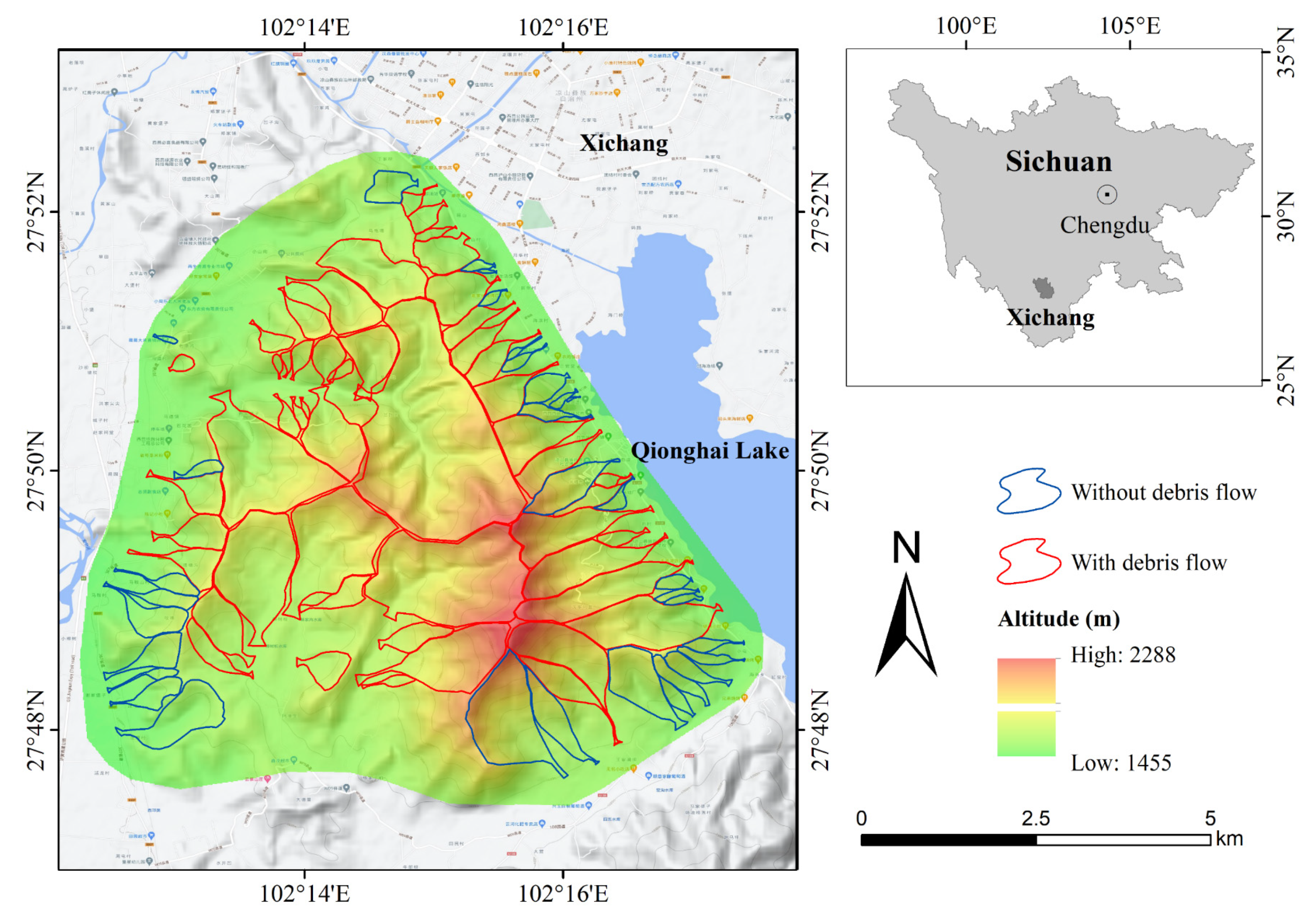
Figure 1. Location of the “30 March 2020” fire burned area and distribution of 82 burned watersheds in Xichang, in which the red line represents the watersheds with post-fire debris flow (greater than or equal to once) and the blue line represents the watersheds without post-fire debris flow (only floods), and the monitoring time is the first post-fire rainy season (May to October 2020).
Remotesensing 14 01306 g001
Figure 2. Fire and PFDFs scene photos of “30 March 2020” in Xichang. (a) Satellite image of the study area before the fire on 1 December 2019 (after Google Earth); (b) forest fire scene photo on 30 March 2020; (c) Satellite image of the study area after the fire on 5 April 2020. The red dotted line is the shooting location of the fire scene in (b), and also the original location of the “30 March 2020” fire in Xichang; (d) The PFDF destroyed downstream houses and roads due to the lack of prevention works in the river watershed on 23 June 2020; (e) The uncompleted debris flow dam is filled due to the debris flow containing large rocks, tree trunks and sediment accumulation blocking the drainage holes on 23 June 2020.
Remotesensing 14 01306 g002
Figure 3. Monthly distribution of rainfall and PFDF occurrence ratio in the study area in 2020.
Remotesensing 14 01306 g003
Figure 4. Characteristics of burned areas: (a) hillslope ash and loose soil layer formed by vegetation burning and high-temperature baking; (b) a large amount of ash and loose sediment deposited at channels and the junction of steep and gentle hillslopes; (c) distribution of dead branches and trunks on channels and hillslopes; (d) distribution of gravel on channels and hillslopes.
Remotesensing 14 01306 g004
Figure 5. The flowchart of this study.
Remotesensing 14 01306 g005
Figure 6. Characteristics and spatial distribution of fire severity in the study area.
Remotesensing 14 01306 g006
Figure 7. The temporal evolution laws of the average of ECE and occurrence frequency of PFDF in 27 rainfall events of the first rainy season after the fire in the study area.
Remotesensing 14 01306 g007
Figure 8. Field investigation of soil water repellence under different vegetation types in burned areas in the study area. WDPT was all measured one hundred times in the soil under different vegetation with the same burned severity. The five water repellency levels in this figure are: wettable (WDPT ≤ 5 s), slightly water repellency (5 s < WDPT ≤ 60 s), strongly water repellency (60 s < WDPT ≤ 600 s), severely water repellency (600 s < WDPT ≤ 3600 s), extremely water repellency (WDPT > 3600 s).
Remotesensing 14 01306 g008
Figure 9. Pearson’s correlation coefficient results, where red represents positive correlation and blue represents negative correlation with increasing magnitude as each color darkens respectively.
Remotesensing 14 01306 g009
Figure 10. The importance of the post-fire debris flow conditioning factors based on the RF method.
Remotesensing 14 01306 g010
Figure 11. Comparison of cross-validation results of 10 candidate models. (a) Validation metrics: AUC and Accuracy, (b) Validation metrics: TS and Sensitivity.
Remotesensing 14 01306 g011
Figure 12. ROC curve and prediction rate for LR model.
Remotesensing 14 01306 g012
Figure 13. Comparison of prediction performance between spatial-temporal prediction model (M) and spatial prediction model (M′). (a) ROC curve comparison, (b) model evaluation metrics comparison.
Remotesensing 14 01306 g013
Figure 14. PFDF susceptibility mapping results of 82 watersheds in the study area in different post-fire periods. (af): susceptibility mapping results of 1 May, 1 June, 1 July, 1 August, 1 September, and 1 October respectively.
Remotesensing 14 01306 g014
Figure 15. Evolution law of percentage of each PFDF susceptibility level in 82 watersheds in the study area over time (number of the post-fire rainstorm events).
Remotesensing 14 01306 g015
Figure 16. Field survey results of PFDF development laws in the first rainy season after the fire. (a) The temporal evolution law of occurrence number of PFDF and its rainfall threshold (max 10 min), (b) the temporal evolution law of cumulative occurrence number of PFDF and its rainfall threshold (max 10 min).
Remotesensing 14 01306 g016
Table 1. Description and source of the influence variables of post-fire debris flow.
VariableDescriptionSource
Watershed morphology charactersArea (km2)Watershed area12.5 m DEM
(ASF, https://search.asf.alaska.edu/, accessed on 12 April 2020)
RR (‰)Relief ratio
WSWatershed shape coefficient
Gradient (°)Watershed average gradient
Slope ≥ 30%Proportion of watershed area with slopes ≥ 30%
Slope ≥ 50%Proportion of watershed area with slopes ≥ 50 %
Fire severityHSProportion of the watershed area burned at high severitySentinel-2 data (20 m pixel size)
M/HSProportion of the watershed area burned at moderate and high severity
Total burnedProportion of watershed area that has been burned
Rainfall
intensity
Max 10 min (mm/h)Maximum 10 min rainfall intensityRadar rain gauges of Xichang Meteorological Bureau
(Every 5 min)
Max 30 min (mm/h)Maximum 30 min rainfall intensity
Max 1 h (mm/h)Maximum 1 h rainfall intensity
Max 24 h (mm)Maximum 24 h rainfall intensity
Hillslope
soil erosion
ECE (mm)The cumulative erosion depth of the hillslope soil
before the PFDF occurs
Field soil erosion monitoring test (5 months, measured after each rainfall)
LE (mm)The erosion depth of the hillslope soil during the
last rainfall
Source
materials
distribution
SMDThe ratio of the supply length of the sediment along the main channel in the watershedField
Investigation
(1 m resolution)
Vegetation distributionVDThe original pine tree coverage area in the watershedField
Investigation
(1 m resolution)
Table 2. Identification criteria of fire intensity in the burnt area: remote sensing interpretation and field investigation of fire intensity characteristics.
Fire SeverityRemote Sensing
Interpretation (dNBR)
Field Characteristics
Unburned<0.12There was no change in the surface cover before and after the wildfire
Low0.12–0.33More than 50% of the litter is incompletely burned
Moderate0.33–0.48Most of the litter is burned; however, most of the crude fuel is incompletely burned
High>0.48Litter and crude fuel are completely burned and the surface is covered with ashes
Table 3. Contingency table.
Observed
Debris FlowNo Debris Flow
PredictedDebris flowTPFP
No debris flowFNTN
Table 4. Validation results of LR model prediction performance.
MetricsAUCSensitivityAccuracyTS
Result0.9350.9640.8870.806
Table 5. Comparison of prediction performance evaluation results of the models established by the balanced and unbalanced sample datasets.
MetricsBalanced Sample ModelUnbalanced Sample ModelD-Value
Sensitivity0.8780.2590.619
AUC0.9220.9070.015
TS0.3030.2150.089
ACC0.8350.922−0.087
Table 6. Percentage of each PFDF susceptibility level in 82 watersheds in the study area in different post-fire periods.
DateNumber of the Post-Fire Rainstorm EventsVery Low
(%)
Low
(%)
Moderate
(%)
High
(%)
Very High
(%)
1 May11.223.6624.3923.1747.56
1 June21.2229.2717.0729.2723.17
1 July78.5426.8328.0534.152.44
1 August1621.9531.7139.027.320.00
1 September2134.1531.7132.931.220.00
1 October2735.3736.5928.050.000.00
Publisher’s Note: MDPI stays neutral with regard to jurisdictional claims in published maps and institutional affiliations.