Article

Smoothing Linear Multi-Target Tracking Using Integrated Track Splitting Filter

1
Department of Defense Systems Engineering, Sejong University, 209 Neungdong-ru, Gwangjin-gu, Seoul 05006, Korea
2
Department of Electrical and Computer Engineering, COMSATS University Islamabad, Abbottabad 22060, Pakistan
3
Department Electronic Systems Engineering, Hanyang University, Ansan 15588, Korea
*
Author to whom correspondence should be addressed.
These authors contributed equally to this work.
Remote Sens. 2022, 14(5), 1289; https://doi.org/10.3390/rs14051289
Submission received: 14 January 2022 / Revised: 26 February 2022 / Accepted: 3 March 2022 / Published: 6 March 2022
(This article belongs to the Special Issue Radar Signal Processing for Target Tracking)

Abstract

:
Multi-target tracking (MTT) is a challenging issue due to an unknown number of real targets, motion uncertainties, and coalescence behavior of sensor (such as radar) measurements. The conventional MTT systems deal with intractable computational complexities because they enumerate all feasible joint measurement-to-track association hypotheses and recursively calculate the a posteriori probabilities of each of these joint hypotheses. Therefore, the state-of-art MTT system demands bypassing the entire joint data association procedure. This research work utilizes linear multi-target (LM) tracking to treat feasible target detections followed by neighbored tracks as clutters. The LM integrated track splitting (LMITS) algorithm was developed without a smoothing application that produces substantial estimation errors. Smoothing refines the state estimation in order to reduce estimation errors for an efficient MTT. Therefore, we propose a novel Fixed Interval Smoothing LMITS (FIsLMITS) algorithm in the existing LMITS algorithm framework to improve MTT performance. This algorithm initializes forward and backward tracks employing LMITS separately using measurements collected from the sensor in each scan. The forward track recursion starts after the smoothing. Therefore, each forward track acquires backward multi-tracks that arrived from upcoming scans (future scans) while simultaneously associating them in a forward track for fusion and smoothing. Thus, forward tracks become more reliable for multi-target state estimation in difficult cluttered environments. Monte Carlo simulations are carried out to demonstrate FIsLMITS with improved state estimation accuracy and false track discrimination (FTD) in comparison to the existing MTT algorithms.

1. Introduction

The target tracking problem in general is a challenging problem due to measurement origin uncertainty. In a multi-target tracking (MTT) system, this complexity is further increased by the problem of measurement coalescence. The measurement origin uncertainty along with coalescence results in producing inaccurate estimates of targets [1]. The MTT system uses moving target indicator sensors such as radar but due to unknown object’s sources (such as real targets, clouds, birds, terrain reflections, etc.) existing in the surveillance region, it is often difficult to identify and detect target source. Thus, target measurements are often misinterpreted because the majority of measurements received by a radar belong to clutters. In this unreliable cluttered environment, the targets have low detection probabilities P D . In addition, tracking filter cannot determine the target trajectories without prior information on position measurements.
A target tracking system initializes tracks using measurements received from the radar. The tracks are recognized as either true (which follow real targets) or false (which follow clutter). Initially, all initialized tracks are referred as false tracks until the suitable tracking algorithm updates the tracks based on the radar measurements in each scan. Therefore, the tracking algorithms use the false track discrimination (FTD) method to measure track quality [2]. An FTD attempts to identify true tracks based on the updated target existence probability (TEP) and eliminate false tracks in each scan. The conventional integrated probabilistic data association (IPDA) algorithm uses TEP as the track quality measure, but it was developed only for single target tracking (STT) situations [3]. The IPDA algorithm propagates and updates only one track state probability density function (pdf) using the single-scan data association procedure. Compared to this, the integrated track splitting (ITS) algorithm produces an exponentially increasing number of track state components with their pdfs and obtains their estimates using multi-scan data association [4]. Thus, ITS is a complex filter, but it is more efficient than IPDA in terms of track retention. The ITS algorithm also provides FTD based on TEP.
The MTT algorithms process measurements originating from multi-targets as well as clutter. In such situations, one measurement of target is often associated with another target (i.e., joint association). Therefore, MTT applies multi-target data association to decide a correct track-to-measurement association assignment in each scan. To incorporate MTT scenario, IPDA and ITS were extended using joint data association based algorithms such as JIPDA [5] and JITS [6], respectively. These algorithms utilize a group of clusters consisting of multi-tracks and associated measurements. Multiple tracks often share measurements. Thus, these algorithms form all measurement-to-track association hypotheses and recursively calculate their a posteriori probabilities of the measurements in each scan. The combinatorial representation in terms of the number of tracks and cluster measurements increases numerical complexities so that these MTT algorithms often exceed the possible computational resources. Similarly to JITS, the multiple hypothesis tracking algorithm evaluates an increasing number of multiple hypotheses followed by a global association that considers all tracks and measurements over a period of scans [7]. Thus, the computation complexity of the multiple hypothesis tracker is greater than JITS algorithm. Moreover, it does not provide any FTD technique. To cope with intractable computational complexities, the linear multi-target (LM) tracking technique was developed based on IPDA (LMIPDA) in [8,9] and based on ITS (LMITS) in [6,8]. The LM method modifies the detected measurements followed by neighbor tracks as clutter measurements in order to obtain state estimates of the current track in each scan cycle. Thus, both LMIPDA and LMITS algorithms allow the MTT system to avoid computations related to the joint measurement hypothesis and joint data association procedure. Therefore, computational complexities in LMIPDA and LMITS algorithms are reasonably limited, even in some scenarios similar to that of STT algorithms. These algorithm employ TEP for track quality measure as well.
The algorithms cited above are referred as non-smoothing algorithms that use only current scan measurements received from a radar to estimate the target state. However, this class of tracking algorithm results in high estimation errors and often limits the accuracy of track quality measures. Smoothing is used to refine the state estimate in current scan k based on state predictions evaluated beyond scan k [2,10]. This involves fusion of forward and backward predictions followed by a two-way tracking from future scan measurements up to and including kth scan measurement. Thus, estimation accuracy and FTD can be significantly improved. The traditional smoothing MTT algorithms, for example, smoothing joint PDA [11], smoothing probability density algorithm [12], and smoothing multiple hypothesis filter [13], do not provide a measure of track quality required for FTD. The fixed interval smoothing based on JIPDA was developed in [14], which extends smoothing data association procedures of previously published algorithms [15,16] to improve multi-target state estimations as well as the FTD. In [17], the authors have used the conventional Rauch–Tung–Striebel [10] in JIPDA, which utilizes forward track measurements to generate corresponding backward tracks for smoothing. As an example of smoothing based on JITS (sJITS), the authors have applied the two-way pass filtering method of the Fraser and Potter algorithm [18] in [19]. In [20], the fixed interval smoothing based on JITS (FIsJITS) was developed for MTT, which outperformed the algorithms developed in [14,17,19]. However, due to involvement of clusters as well as ITS multi-track components, the joint data association procedure in FIsJITS and sJITS is computationally intensive and complex. With the development of state-of-art MTT systems, fixed interval smoothing based on LMIPDA (FLsLMIPDA) algorithm was developed with the integration of the LM technique in [21,22].
In order to incorporate an extended number of unknown targets, we propose fixed interval smoothing using LMITS (FIsLMITS). Assuming fixed interval [ k , N ] , where k is the first scan and N is the last scan index of subsequent intervals, FIsLMITS initializes and estimates backward multi-tracks using measurements collected by sensor in each scan (from Nth scan up to kth scan), which does not correspond to any forward tracks. This implies that target state estimate is calculated up to and including scan k. For smoothing, FIsLMITS initializes tentative forward multi-tracks using the measurements received from the sensor and develops the validation gate in scan k assuming backward multi-track–multi-components state prediction as measurements in the forward path track. Thus, backward multi-tracks are not fused until they fall in the validation gate of the forward track. Each forward track state component fuses with the associated backward state components to obtain multiple smoothing components prediction. The a posteriori probabilities of these predicted smoothing components are evaluated using modified clutter measurement density to obtain smoothing component data association probabilities in each scan k. The predicted smoothing components select the smoothing validation measurements from the set of sensor measurements to obtain multi-target state estimation of FIsLMITS track as well as forward track in each scan k. This implies that a forward track is also refined using the smoothing, and it becomes robust due to the smoothing in each subsequent scan in the fixed interval. The smoothing target existence probabilities are also calculated to measure the track quality in each scan k for FTD.
The main contribution of the proposed FIsLMITS algorithm is the integration of LMITS framework with the fixed interval smoothing algorithm, thus improving multi-target state estimation in cluttered environments. Unlike the existing fixed interval smoothing algorithms such as [17,19], the proposed novel FIsLMITS algorithm fetches radar measurements from future scans by employing a backward-running LMITS filter so that a priori smoothing platforms could be anticipated for a forward track in past scan k. With the proposed method, smoothing is achieved only when the backward multi-track–multi-components fall in the validation gate of the forward track. Thus, the proposed smoothing idea refines the state estimate of forward track for a significant improvement in FTD.
The target and sensor models are developed in Section 2. Section 3 proposes the novelty and method of the FIsLMITS algorithm. The statistical analysis of the FIsLMITS algorithm is compared to the existing MTT algorithms based on the ITS family such as FIsJITS, sJITS, LMITS, and FIsLMIPDA and LMIPDA in Section 4. Finally, the discussion on the FIsLMITS results is concluded in Section 5.

2. Target and Sensor Models

Assume that target existence χ k τ is a random event and target trajectory state x k τ is a random variable, where τ represents an index of a target as well as a track and k indicates an index of a scan. The target source (such as unmanned aerial vehicle (UAV)) produces at most one measurement per scan with detection probability, P D . In the two-dimensional surveillance region, the target (UAV) consists of a two-dimensional position and velocity vectors. The motion equation of the target trajectory state is derived using state transition matrix F k , which is used to propagate the state vector from scan k 1 to scan k, which is as follows:
x k τ = F k x k 1 τ + v k 1 ,
where v k 1 is the target white Gaussian noise, which has a zero-mean and a known covariance matrix Q k . The matrices of F k and Q k are expressed in [2,10], and they are repeated here for clarity:
F k = I 2 × 2 T I 2 × 2 O 2 × 2 I 2 × 2 ,
Q k = q 0.25 T 4 I 2 × 2 0.5 T 3 I 2 × 2 0.5 T 3 I 2 × 2 T 2 I 2 × 2 ,
where I 2 × 2 is the 2 × 2 identity matrix, O 2 × 2 is the 2 × 2 zeros matrix, T denotes the sensor scan time, and q denotes the white noise acceleration uncertainty that is also known as process noise.
If the target is identified and detected by a radar with P D in scan k, then the equation of sensor position measurement of the target state is derived using a measurement matrix, H k = [ I 2 × 2 , O 2 × 2 ] , in the following:
Z k τ = H k x k τ + w k ,
where w k denotes the white noise of the position measurement which has a zero-mean and a known covariance matrix R k . Other than target measurements, a radar also observes a random number of clutter measurements. These clutter measurements are generated using the nonhomogeneous Poisson distribution process [23]. Let Z k be the set of measurements with cardinality M k received in scan k and Z k = Z k , Z k + 1 , , Z N be the cumulative set of fixed measurement interval which starts from first scan k and ending with last scan N, which is the measurement set of an interval. This fixed interval is the sequence of measurement sets received from consecutive scans. In the cluttered environment, target measurement Z k τ is often misinterpreted because the source of each measurement in Z k is not known. The density of clutter measurements denoted by ρ k is assumed to be known, which is a function of M k measurements specified in the X and Y coordinates of Z k . For example, the density of the ith measurement Z k , i of the measurement set equals ρ k , i ρ Z k , i .

3. Fixed Interval Smoothing in Linear Multi-Target Based on ITS (FIsLMITS)

This manuscript extends the non-smoothing LMITS algorithm by using the smoothing data association idea to improve the weakness of LMITS for tracking the motion of multi-targets in the cluttered environment. The proposed FIsLMITS algorithm applies the fixed measurement interval approach [24] for smoothing. Each fixed interval [ k , N ] has N k + 1 scans, for example, if the first interval starts at k = 1 and ends at N = 8 ; then, the interval length becomes 8. Each fixed interval follows three steps:
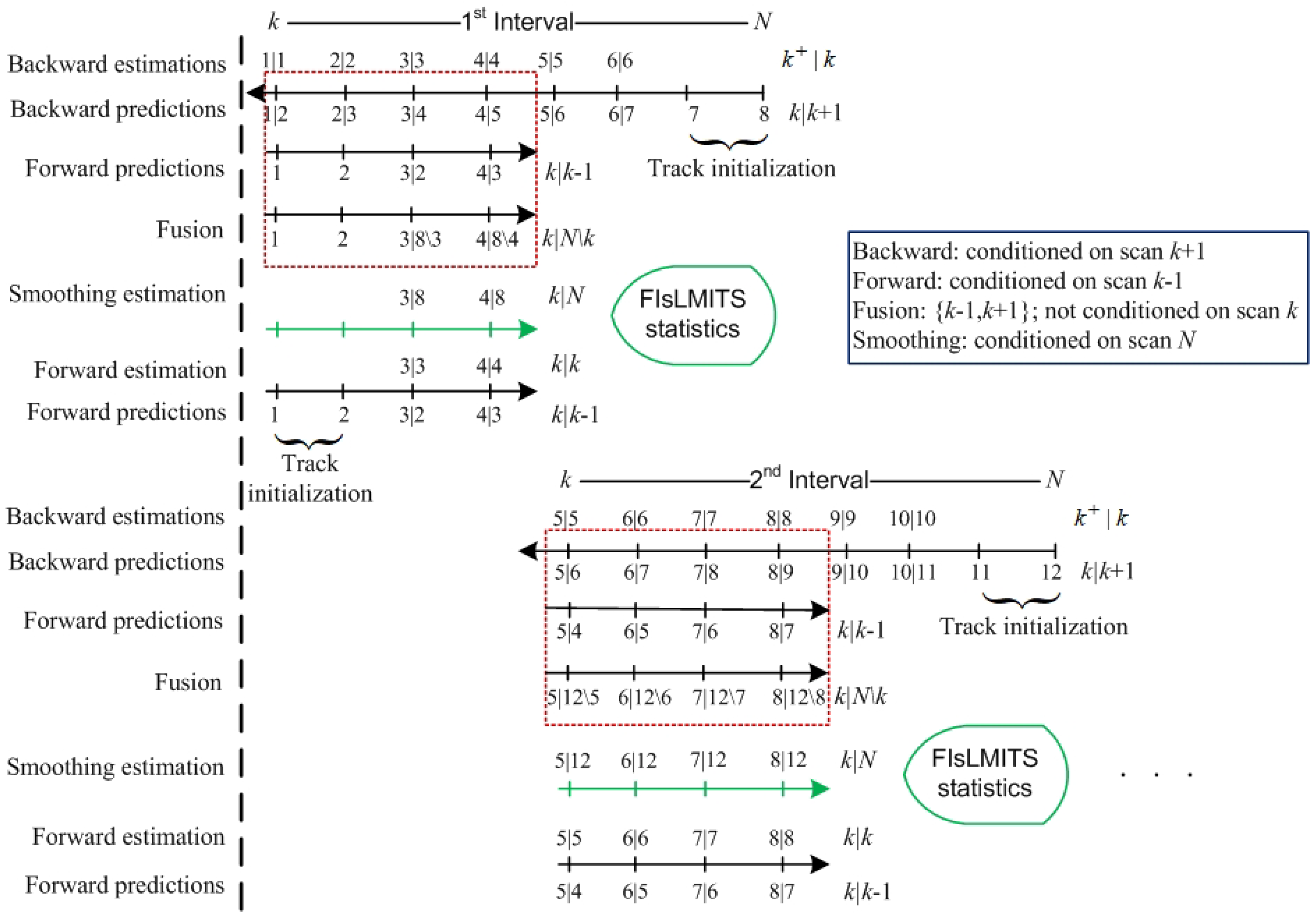
  • Calculate the backward multi-tracks multi-components state estimations from scan N up to scan k based on the measurements Z k + received in each scan k + (where subscript k + on Z k + indicates the backward-time scan).
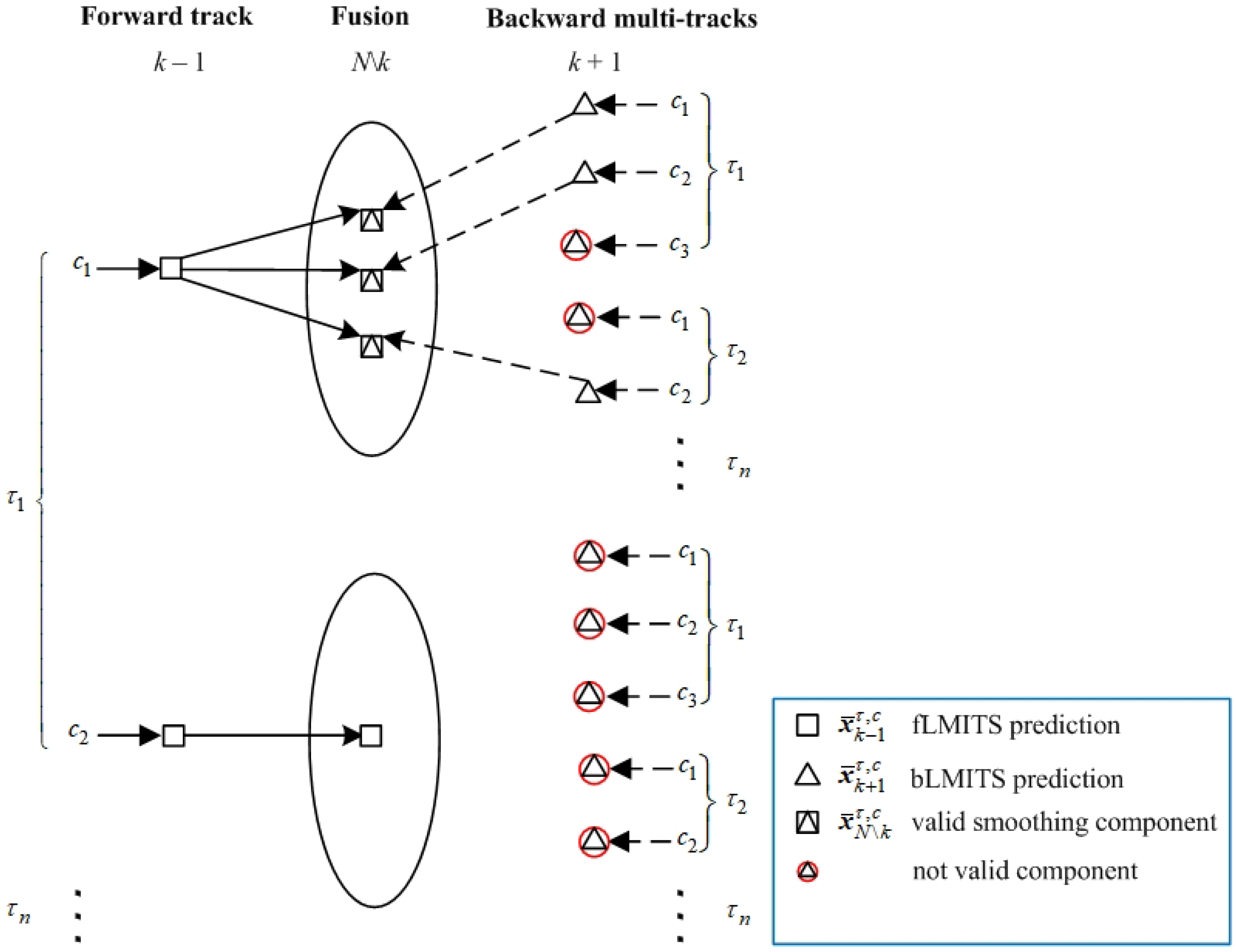
  • After the arrival of the backward multi-tracks at first scan k of an interval, the forward multi-tracks are initialized using the corresponding component pdf measured by the sensor measurements. Each forward track forms a validation gate based on the backward multi-track-multi-components predictions. In the validation gate, each forward component prediction fuses with the associated backward multi-components predictions to obtain the smoothing multi-components predictions in each scan k (for example, x ¯ 3 | 8 \ 3 τ , c ).
  • Calculate the smoothing and forward estimates using the step 2 in each scan k, for example, x ^ 3 | 8 τ and x ^ 3 | 3 , i τ , c , respectively.
Thus, the estimates of forward track components are refined in a smoothing fashion to make the smoothing track more robust for multi-target tracking in clutters. Consequently, the forward and smoothing estimates are computed recursively in each scan k of the fixed interval [ k , N ] . To verify the robustness of FIsLMITS, the smoothing probability of the potential target existence is also calculated in each scan k, which is used as a performance parametric to measure the track quality as well as FTD. Figure 1 illustrates the fixed interval smoothing implementation of the FIsLMITS algorithm.
In each scan k, the existing forward tracks are concatenated with newly initialized forward tracks for subsequent fusion and smoothing. Thus, an FIsLMITS filters two types of information: smoothing and forward state estimates followed by fusion in each scan k. To obtain a maximum smoothing performance, the next interval is overlapped to the current interval, for example, the next interval includes k = 5 , 6 , , 12 scans as depicted in Figure 1. In other words, the FIsLMITS smoothing statistics are accumulated for the first four scans only, and the rest of measurement scans are overlapped to the next four consecutive scans. This smoothing process limits the significant smoothing-time delay and reduces position estimation errors.

3.1. Backward Multi-Track State Estimation

The LMITS algorithm is applied in the reverse-time measurements sequence from Nth scan to kth scan using the fixed interval set Z k . The two-point measurement difference technique [2] is utilized, which uses each pair of measurement from two consecutive scans to generate a backward track. For example, an ith pair of measurement Z N , i , Z N 1 , i initializes a backward track in scan N 1 using a generalized two-point position difference formula expressed in (5). Similarly, an ith pair of measurement Z k , i , Z k + 1 , i initializes a backward track in scan k + 1 using following constraint:
V k + 1 , i = X k + 1 , i X k , i 2 + Y k + 1 , i Y k , i 2 T V m a x ,
where V k + 1 , i is the resultant velocity of the ith measurement calculated in scan k + 1 using coordinates X k + 1 , i , X k , i , Y k + 1 , i , and Y k , i of the ith measurement of the two consecutive scans, V m a x represents the target maximum velocity, and (−) sign with the T implies the reverse-time backward scanning. Thus, backward track recursion starts from scan k + 1 with the updated component state pdf p χ k + 1 τ , x k + 1 τ , c | Z k + 1 = Z k + 1 , V k + 1 and component existence probability ζ k + 1 τ , c (where superscript c denotes a component index), which initially equals to 1. In addition, each track has an initial target existance probability (TEP) and a unique track identity number. The component state pdf is updated using Kalman Filter update equations [25] to obtain the backward track state prediction in scan k conditioning on measurements Z k + 1 and on scan k + 1 , which is as follows:
x ¯ k | k + 1 τ , c = F k 1 x ^ k + 1 | k + 1 τ , c P ¯ k | k + 1 τ , c = F k 1 P ^ k + 1 | k + 1 τ , c F k t + Q k * ,
where the cap-accent on x ^ k + 1 | k + 1 τ , c and on P ^ k + 1 | k + 1 τ , c represents the state estimate and its covariance, respectively, the bar-accent on x ¯ k | k + 1 τ , c and on P ¯ k | k + 1 τ , c represents state prediction and its covariance, respectively, superscript t on F k indicates the inverse transpose, and Q k * = F k 1 Q k F k t denotes the the covariance matrix of the backward state trajectory. It is noted that the inverse and inverse transpose terminologies on matrix F k implies the perception of backward tracking.
The Markov Chain One model of the target existence is applied to update and maintain the track quality measure given the prior probability of target existence with respect to track τ [2,3] expressed as follows:
P { χ k τ Z k + 1 } = α P { χ k + 1 τ Z k + 1 } ,
where α denotes the target state transition probability that is used to update the prior TEP with respect to τ th track from scan k + 1 to current scan k.
The validation measurement criterion [2] is applied to each measurement of set Z k to select the component validation measurement z k , i τ , c associated with a backward component state prediction within a predetermined maximum gating threshold, which is as follows:
Z k , i H k x ¯ k | k + 1 τ , c t S k 1 Z k , i H k x ¯ k | k + 1 τ , c γ ,
where S k = H k P ¯ k | k + 1 τ , c H k t + R k represents the covariance of the measurement innovation and γ denotes the maximum threshold that selects component validation measurements z k , i τ , c from Z k . The value of the selection threshold is determined by the probability of the validation gate, that is, P G = 1 e 0.5 γ , where the value of P G should be at the maximum, such as 0.99. Therefore, the set of selected component measurements corresponding to backward track τ is accumulated by the following.
z k τ = c z k , i τ , c .
The likelihood of the validated component measurement z k , i τ , c with respect to the backward component prediction of the τ th track is calculated by the following.
p k , i τ , c = 1 2 π S k e 0.5 z k , i τ , c H k x ¯ k | k + 1 τ , c t S k 1 z k , i τ , c H k x ¯ k | k + 1 τ , c .
The backward track likelihood p k , i τ of the ith validated measurement z k , i τ (obtained in Equation (9)) is calculated by the following.
p k , i τ = c ζ k + 1 τ , c p k , i τ , c .
For tracking the τ th target, the LM technique avoids the influence of other targets while treating them as clutters. Thus, LM calculates the probabilistic weight P k , i τ of the τ th target to assure that the selected measurement z k , i τ is the τ th target by using the following:
P k , i τ = P D P G P { χ k τ Z k + 1 } p k , i τ / ρ k , i i = 1 m k p k , i τ / ρ k , i ,
where m k denotes the number of validation measurements selected by (8). Equation (12) determines the mutual exclusiveness of the prior probabilities of detected target measurements; thus, only one measurement corresponds to the potential target. If there are no measurements ( i = 0 ) selected by (8), that is, all measurements fall outside the validation gate, then p k , i τ , c = p k , i τ = P k , i τ = 0 . The tracks σ other than the τ th target track are treated as modified clutter-tracks; therefore, they correspond to the modified clutter measurement densities by the following:
μ k , i τ = ρ k , i + σ = 1 σ τ σ = τ n p k , i σ P k , i σ 1 P k , i σ ,
where modified clutter measurement density μ k , i τ is calculated at the coordinates of the detected measurement z k , i τ being observed by a τ th track, τ n denotes the total number of tracks, and the term in parentheses at the denominator represents the probability that the target does not exist in the neighbored tracks σ ( σ τ ) . The backward-running LMITS filter applies Equation (13) to calculate likelihood ratio λ k τ and the multi-target component data association probabilities of measurements z k , i τ corresponding to each track τ . These are expressed, respectively, by the following:
λ k τ = 1 P D P G + P D P G i > 0 p k , i τ μ k , i τ ,
and the following is the case.
β k , i τ , c = P D P G p k , i τ λ k τ μ k , i τ .
However, Equations (14) and (15) become equal to 1 P D P G and 1 P D P G / λ k τ , respectively, for i = 0 . The backward track τ th TEP conditioning on measurements Z k + and on scan k + is estimated by using the following.
P χ k + τ | Z k + = λ k τ P χ k τ | Z k + 1 1 1 λ k τ P χ k τ | Z k + 1 ,
Each feasible validated component measurement z k , i τ , c selected in scan k creates a new track component with a component existence probability expressed as follows.
ζ k + τ , c = β k , i τ , c ζ k + 1 τ , c 1 ; i = 0 p k , i τ , c p k , i τ ; i > 0 ,
The backward LMITS algorithm applies Kalman Filter estimation equations [25] to backward track components based on backward validated component measurements z k , i τ , c in order to calculate its components state estimation with respect to τ th track in scan k by using the following:
x ^ k | k + , i τ , c = x ¯ k | k + 1 τ , c + K k Z k , i τ , c H k x ¯ k | k + 1 τ , c P ^ k | k + , i τ , c = P ¯ k | k + 1 τ , c K k H k P ¯ k | k + 1 τ , c ,
where K k = P ¯ k | k + 1 τ , c H k t S k 1 denotes the gain of the Kalman Filter at scan k. In the next scan k, each estimated backward component with respect to track τ is retrieved from scan k + 1 and updated using Equation (6), which is used to obtain the component state prediction and its covariance represented by x ¯ k | k + 1 τ , c and P ¯ k | k + 1 τ , c , respectively. Similarly, the backward LMITS recursively calculates the multi-track backward state components as well as the TEP of the multi-tracks using Equations (6)–(18) in each scan k.

3.2. Backward Multi-Track State Fusion in a Forward Track

This section discusses the fusion of backward multi-tracks state components in a forward track. Similarly to the initialization process of backward tracks, the tentative forward tracks are initialized based on feasible gated measurements Z k , i selected by (5). Thus, each paired measurement from two consecutive scans Z k = { Z k , Z k 1 } initializes a track in scan k 1 . Thus, each forward LMITS track is initialized with an initial TEP P { χ k 1 τ | Z k 1 } , a state component pdf p { χ k 1 τ , x k 1 τ , c | Z k 1 } , and an initial component existence probability, ζ k 1 τ , c = 1 . The forward track updates and propagates the τ th TEP from scan k 1 to the next scan k and obtains the updated TEP P { χ k τ | Z k 1 } at scan k by shifting the time-sequence subscript from k + 1 to k 1 in (7). The forward track state component pdf is updated based on Z k 1 in scan k 1 , which propagates linearly in each scan using the following Kalman Filter propagation equation.
x ¯ k | k 1 τ , c = F k x ^ k 1 | k 1 τ , c P ¯ k | k 1 τ , c = F k P ^ k 1 | k 1 τ , c F k t + Q k .
Unlike the existing MTT algorithms [17,19,22], the recursion of the forward track is followed by a smoothing estimation, which is obtained by fusing backward multi-tracks components to each tentative forward track component. Thus, a forward component develops a validation gate exploiting the set of backward multi-track-multi-components state prediction p { χ k + 1 τ , x k + 1 τ , c | Z k + 1 } τ n as a set of measurements. This implies that each forward track is conditioned on a set of backward multi-components. Each forward state component forms a certain number of true pairs in association with backward multi-tracks components using the validation measurement selection criterion expressed in (20). This procedure is illustrated in Figure 2.
x ¯ k | k + 1 τ , c x ¯ k | k 1 τ , c T P ¯ k | k + 1 τ , c P ¯ k | k 1 τ , c 1 x ¯ k | k + 1 τ , c x ¯ k | k 1 τ , c γ .
In Figure 2, assume that a forward track τ 1 has two components with state pdf c 1 and c 2 as indicated by ’squares’, whereas backward track τ 1 has three components ( c 1 , c 2 , and c 3 ), τ 2 has two components ( c 1 and c 2 ), and so on, as indicated by ’triangles’. Forward track component c 1 makes a certain number of true pair of fusion components in association with backward components, as depicted in Figure 2.
The forward track component, for example, c 1 (Figure 2), uses information fusion filter equations [26,27] to calculate the a priori smoothing component state prediction with respect to the validated backward track as expressed by:
x ¯ k | N \ k τ , c = P ¯ k | N \ k τ , c P ¯ k | k 1 τ , c 1 x ¯ k | k 1 τ , c + P ¯ k | k + 1 τ , c 1 x ¯ k | k + 1 τ , c ,
where P ¯ k | N \ k τ , c denotes the associated a-priori smoothing component state covariance:
P ¯ k | N \ k τ , c 1 = P ¯ k | k + 1 τ , c 1 + P ¯ k | k 1 τ , c 1 ,
where subscript N \ k indicates that the fused component is not conditioned on sensor measurements (i.e., k is excluded from N). However, if none of the backward multi-track components satisfy (20), then the component fusion state prediction becomes a corresponding forward state component prediction. For example, the forward track component c 2 does not select any backward track component in its validation gate as depicted in Figure 2 so that the a prior smoothing state component prediction and its covariance becomes [ x ¯ k | N \ k τ , c , P ¯ k | N \ k τ , c ] = [ x ¯ k | k 1 τ , c , P ¯ k | k 1 τ , c ] .
The likelihood of fused component p k τ , c associated with τ th validated backward track component is calculated by using the following:
p N \ k , i τ , c = 1 2 π s k e 0.5 x ¯ k | k + 1 τ , c x ¯ k | k 1 τ , c t s k 1 x ¯ k | k + 1 τ , c x ¯ k | k 1 τ , c ,
where s k = P ¯ k | k + 1 τ , c + P ¯ k | k 1 τ , c represents the covariance of fused measurement innovation. Equation (23) is used to calculate the likelihood of the τ th fusion track by the following.
p N \ k , i τ = k 1 c k + 1 c ζ k + 1 τ , c ζ k 1 τ , c p N \ k , i τ , c .
However, if the τ th backward track is not selected by (20), then the fused component and fused track likelihoods become zero (i.e., p N \ k , i τ , c = p N \ k , i τ = 0 ). Assume that P D τ = 1 1 P D N k + 1 denotes the probability that the τ th target is detected by the fusion track and exist either in scan k + 1 or k 1 in the interval [ k , N ] . Furthermore, assume that the density of the backward tracks per cross-sectional area A of the surveillance region is d k , i = τ n / A . Based on these assumptions, the likelihood ratio of the fusion track λ N \ k τ is derived as follows:
λ N \ k τ = 1 P D τ P G + P D τ P G i > 0 p N \ k , i τ d k , i ,
which is used to calculate the a priori smoothing target existence probability as follows.
P χ k τ | Z N \ k = Λ N \ k τ P χ k τ | Z k 1 P χ k + τ | Z k + 1 1 Λ N \ k τ P χ k τ | Z k 1 P χ k + τ | Z k + ,
In Equation (26), the original formulae of TEP [2,3,4] is modified using the proposed FIsLMITS algorithm, which utilizes the τ th backward TEP to update the a priori smoothing TEP (i.e., TEP of the fusion track). Because the potential τ th target was already detected and its state estimate was calculated in the kth scan using (18), each feasible true pair of fusion component has an a priori smoothing component existence probability, which is calculated by using the associated backward component existence probability in Equation (27). Based on the above assumptions, we have the following:
ζ N \ k τ , c = ζ k 1 τ , c Λ N \ k τ 1 P D τ P G ; i f τ i s n o t v a l i d a t e d t r a c k P D τ P G ζ k + 1 τ , c p N \ k , i τ , c d k , i ; i f τ i s v a l i d a t e d t r a c k .

3.3. Forward Track State Estimation Using Smoothing Multi-Target Data Association

This section derives the multi-target state estimations corresponding to the forward tracks that require the smoothing multi-target component state estimations, the component validation measurements, and their data association probabilities. For the sake of simplicity, apply the same notations of current track τ and neighbored tracks σ in the smoothing tracks. The predicted smoothing state component and associated state covariances obtained from Equations (21) and (22) develop a validation gate around the smoothing component validation measurements z ´ k , i τ , c (where an acute accent indicates smoothing) that are selected from sensor measurements Z k in scan k. Utilizing the validation selection method, we have the following:
Z k x ¯ k | N \ k τ , c t S ´ k 1 Z k x ¯ k | N \ k τ , c γ ,
where S ´ k = H k P ¯ k | N \ k τ , c H k t + R k denotes the measurement innovation covariance. Each predicted smoothing component and a feasible smoothing validated measurement produce a smoothing component with component likelihood p ´ k , i τ , c expressed by the following:
p ´ k , i τ , c = 1 2 π S ´ k e 0.5 z ´ k , i τ , c H k x ¯ k | N \ k τ , c t S ´ k 1 z ´ k , i τ , c H k x ¯ k | N \ k τ , c ,
which calculates the smoothing track likelihood p ´ k , i τ of the selected smoothing measurement by using the following.
p ´ k , i τ = c ζ N \ k τ , c p ´ k , i τ , c .
The a priori smoothing probability in which the selected smoothing measurement z ´ k , i τ , c is the detected τ th target measurement being followed by a track τ is evaluated by the following.
P ´ k , i τ = P D P G P { χ k τ Z N \ k } p ´ k , i τ / ρ k , i i = 1 m ´ k p ´ k , i τ / ρ k , i .
In the FIsLMITS smoothing track’s τ update step, smoothing clutter measurement density is modulated by using Equations (30) and (31) in the following:
μ ´ k , i τ = ρ k , i + σ = 1 σ τ σ = τ n p ´ k , i σ P ´ k , i σ 1 P ´ k , i σ ,
which is used to compute the smoothing track likelihood ratio and smoothing multi-target components data association probabilities, as expressed by the following:
λ ´ k τ = 1 P D P G + P D P G i > 0 p ´ k , i τ μ ´ k , i τ ,
and the following is the case.
β ´ k , i τ , c = P D P G p ´ k , i τ λ ´ k τ μ ´ k , i τ .
Each feasible validated smoothing measurement (selected by Equation (28)) and the associated smoothing component predictions (obtained from Equation (21)) produce a new component with a smoothing component existence probability that is calculated by using Equation (34) in the following:
ζ ´ k | N τ , c = ζ N \ k τ , c β ´ k , i τ , c p ´ k , i τ , c p ´ k , i τ ,
where subscript k | N indicates that the component is smoothed in the kth scan using the measurement from Nth scan up to kth scan (i.e., conditioning on measurements Z N ). Equation (26) is modulated by using the smoothing track likelihood ratio to estimate the FIsLMITS-smoothing TEP of the potential τ th target, which is the following.
P χ k τ | Z N = λ ´ k τ P χ k τ | Z N \ k 1 1 λ ´ k τ P χ k τ | Z N \ k .
FIsLMITS utilizes Kalman Filter estimation equations ( KF est ) to estimate the smoothing component state in scan k conditioning on measurement Z N by using the validated smoothing component measurements z ´ k , i τ , c in the following:
x ^ k | N , i τ , c , P ^ k | N , i τ , c = x ¯ k | N \ k τ , c , P ¯ k | N \ k τ , c ; i = 0 KF est Z ´ k , i τ , c , R k , x ¯ k | N \ k τ , c , P ¯ k | N \ k τ , c ; i > 0 ,
which is approximated by one Gaussian state pdf mean and its covariance using the Equation (35) in the following:
x ^ k , N τ = c ζ ´ k | N τ , c x ^ k | N , i τ , c
and the following is the case:
P ^ k , N τ = c ζ ´ k | N τ , c P ^ k | N , i τ , c + x ^ k | N , i τ , c x ^ k | N , i τ , c t x ^ k , N τ x ^ k , N τ t ,
where subscript k , N implies that the smoothing track state pdf is obtained at scan k given the measurements up to N scans. The above smoothing Equations (38) are used recursively for FIsLMITS track output statistic computation in each scan k.
The recursion of the forward-running LMITS filter starts after the smoothing achieved in the kth scan. The proposed FIsLMITS algorithm does not apply the LM method for multi-target data association evaluations in the forward tracks. Hence, it minimizes computational time and resources. In fact, FIsLMITS utilizes the validated smoothing measurements, modulated smoothing clutter measurement densities, and smoothing multi-target data association probabilities to calculate the forward track likelihoods, state estimations, and TEPs. Thus, the forward tracks become more robust with the help of smoothing measurements collected up to kth scan so that they become applicable even for the toughest MTT situations. To deal with multi-target data association situations in the forward tracks, the track component measurement likelihood of z ´ k , i τ , c corresponding to the propagated forward component state prediction (obtained from Equation (19)) is calculated by using the weighted product of the smoothing component data association probabilities in the following:
p k , i τ , c = β ´ k , i τ , c 2 π S k e 0.5 z ´ k , i τ , c H k x ¯ k | k 1 τ , c t S k 1 z ´ k , i τ , c H k x ¯ k | k 1 τ , c ,
where S k = H k P ¯ k | k 1 τ , c H k t + R k represents the measurement innovation covariance of a forward track in scan k. To avoid the use of repeated equations, consider the same nomenclature in forward tracking as that used in backward tracking.
Equation (11) is applied with subscript k 1 on ζ k 1 τ , c (replacing the subscript k + 1 on ζ k + 1 τ , c ) to obtain the forward track likelihood p k , i τ . For forward track updates, the track likelihood ratio λ k , i τ is calculated using μ ´ k , i τ (replacing μ k , i τ ) in Equation (14), which is used to compute the a posteriori TEP P { χ k τ | Z k } corresponding to the potential τ th target in forward-time scan k. Replacing the time-sequence subscript k + 1 by k 1 on p { χ k τ | Z k 1 } in Equation (16), we obtain the a posteriori TEP P { χ k τ | Z k } in scan k. Each feasible smoothing validated component measurement and a predicted forward track state component develops a new component with component existence probability that is calculated in a similar fashion as in Equation (35), and we have the following.
ζ k τ , c = ζ k 1 τ , c β ´ k , i τ , c p k , i τ , c p k , i τ ,
Finally, Equation (37) is used with the time-sequence subscript k 1 on x ¯ k | k 1 τ , c and on P ¯ k | k 1 , i τ , c (replacing x ¯ k | N \ k τ , c and P ¯ k | N \ k τ , c ) to calculate the forward track multi-components state estimates and their covariances represented by x ^ k | k , i τ , c and P ^ k | k , i τ , c , respectively. Similarly, Equation (19) is applied to propagate the state estimates of the forward track components to the next scan k, where the consequence of fusion and smoothing is to be performed in smoothing interval [ k , N ] . Thus, the FIsLMITS smoothing track state estimates obtained from (38) becomes significantly improved for an efficient tracking of the potential targets in each scan k, following the recursive equations from (5) to (41).

4. Numerical and Technical Analysis Using Simulations

This section discusses the numerical and technical analysis of the proposed FIsLMITS algorithm in comparison to existing MTT smoothing/non-smoothing algorithms such as FLsLMIPDA, FIsJITS, sJITS, LMITS, and LMIPDA.

4.1. Technical Considerations

The FIsLMITS algorithm utilizes track component pruning and merging techniques [2,28,29] in forward and backward tracks in order to limit the exponentially increasing number of components. It is not required to apply these techniques in smoothing tracks because they do not propagate. The FIsLMITS algorithm uses a predetermined pruning threshold to eliminate track components corresponding to their low component existence probabilities. In addition, the component merging technique compares the component measurement histories accumulated in the last four scans in order to merge identical components. Identical track components are merged to one Gaussian pdf mean accompanying by its covariance, thereby reducing the computational complexities in multi-target data association evaluation. The FIsLMITS, FIsJITS, and sJITS algorithms apply the same pruning threshold as well as same merging technique in this manuscript for a fair comparison.
Since, a track is always tentative; therefore, the confirmation of the tracks is required. The FIsLMITS uses predetermined track confirmation and termination thresholds to determine the nature of the forward, backward, and smoothing tracks based on their updated TEPs. In the case of smoothed tracks, it uses smoothing TEP as a track quality measure for FTD evaluation. A confirmed track should exceed a confirmation threshold; otherwise, it could be terminated if its updated TEP falls below a termination threshold value. Moreover, a confirmed track remains confirmed regardless of the updated TEP until its termination. Therefore, the TEP of forward, backward, and smoothing tracks is updated recursively in each scan k to determine track quality measures. In the cluttered environment, a confirmed track may often follow the clutters. FIsLMITS applies the chi-squared statistical test [2,10] to verify the confirmed tracks that is defined by the following:
x ^ k , N τ x k τ T P 0 | 0 τ 1 x ^ k , N τ x k τ < η ,
where P 0 | 0 τ represents the initial covariance of target measurement noise sequence and η denotes the true track selection threshold of the statistical condition, which depends on the false-alarm probability distribution [2,10]. If a confirmed track satisfies Equation (42) with a threshold 20 ; then, it is referred to as a confirmed true track (CTT); otherwise, it is a confirmed false track (CFT). Moreover, a CTT may become a CFT due to the presence of clutters and other targets if it exceeds false condition threshold 40 . These threshold values are dependent on the target model, target velocities, and area of surveillance region. This statistical test is evaluated between each confirmed track state estimate (Equation (38)) and each target state (Equation (1)) in each scan k.
Moreover, it is also possible that a potential target is followed by more than one CTT, although only one CTT is required for tracking the corresponding targets. Therefore, the FIsLMITS algorithm utilizes the auction algorithm [30], which is used to bid for asynchronous CTTs. The auction algorithm measures the benefit score which calculates the minimum normalized distance squared value ( x ^ k , N τ x k τ ) with respect to each CTT τ . Then, the benefit score evaluates the winning bid with respect to each CTT. A bid is placed when the τ th benefit score is greater than any other bid of CTT. Therefore, the auction algorithm is explicitly used for selecting only one CTT corresponding to the potential target with the highest winning bid.

4.2. Simulation Parameters and Scenario

Assume that the smoothing algorithms FIsLMITS, FIsLMIPDA, FIsJITS, and sJITS have the same measurement interval length. Each smoothing/non-smoothing algorithm was initialized with the same TEP (i.e., 0.01 ) and has a same track termination threshold (same value as initial TEP) for a fair comparison. However, only the confirmation threshold was tuned to obtain a similar number of CFTs (≈25).
This research work was conducted using 200 Monte Carlo simulation runs in the two-dimensional surveillance region that has a [ 700 ; 700 ] m dimension along X and Y axes. Each simulation run consists of 36 scans with sampling interval time T = 1 s. In this region, the sensor (e.g., radar) returns the random number of clutters processed by the Poisson distribution in each scan with a measurement density of ρ k , i τ = 0.0001 . These measurements are additionally corrupted by sensor noise with known covariance R k = 25 I 2 × 2 m 2 . Thus, the average number of clutters observed in each scan k equals 48. In this cluttered environment, each algorithm generated around 120,548 (603 per run) forward tracks. In addition to this, the backward tracks of FIsLMITS, FIsLMIPDA, and FIsJITS were initialized roughly around 167,380 (837 per run); therefore, they consumed more computational time in comparison to that of non-smoothing algorithms. We assumed a maximum target velocity of 25 m / s for track initialization using Equation (5) (i.e., two-point initialization process). Each algorithm applies target model state transition probability ( α = 0.98 ) followed by Markov Chain One target existence event [3] in order to update and maintain track propagation in each scan k. Moreover, the target model was also corrupted with a process noise of q = 0.75 m 2 / s 4 and has a detection probability, P D = 0.9 . We assumed that each target is untagged and has been shuffled by clutter measurements with density ρ k , i τ . Only the target initial position without its velocity information is known to each algorithm. Given the Table 1, we have the following.
The FIsLMITS algorithm is implemented for tracking and estimating the state of six targets in clutters, as shown in Figure 3. For reasons of simplicity and clarity, this figure illustrates the smoothing trajectories of targets from one simulation run. The targets are moving very closely near the intersection point of the coordinates and certainly crossing at approximately [ 387 ; 300 ] m at different times. It is assumed that each target moves uniformly at a different corresponding velocity and has a different flight angle. Due to this, the measurement of one target is often associated with other targets near the intersection point.
Table 2 shows the statistics of the multi-track retention accounting from 200 simulation runs that are accumulated before and after crossing of the multi-targets. Each algorithm preserves the index of multi-track for statistics evaluation. The track retention has following important parameters:
  • nCases: It is the number of CTTs following a potential target that was counted in scan 15;
  • nOk: The number of CTTs that keep pursuing the original target (without switching to other target track) in scan 30;
  • nSwitched: It counts the number of CTTs that swapped the original target and are now pursuing a different target in scan 30;
  • nLost: The number of CTTs accounted from nCases that are not pursuing any target in scan 30 because they were terminated due to low track TEP or low track component existence probabilities or they became confirmed false tracks;
  • nResult: It counts the number of CTTs that is retained until the last scan k = 36 .
Table 2 shows that the proposed FIsLMITS algorithm produces the highest number of nCases and nOk, and the lowest number of nSwitched and nLost. It is noted that the number of nLost is not necessarily the same as the number of CFTs. Table 2 also compares the algorithms in terms of execution time per run. The standard ITS filter is computationally expensive due to an exponentially increasing number of track components. Additionally, under the joint measurement assumption, the FIsJITS and sJITS consumed a large amount of computation time in each run as compared to the linear multi-target based algorithms. The proposed FIsLMITS algorithm invested only 1.52 s in each run and earned significant performance in terms of multi-track retention. The LMIPDA algorithm is the simplest among the existing algorithms, which utilizes the standard IPDA algorithm; therefore, it has a lowest execution time per run. Moreover, operating the FIsJITS and sJITS for the estimation of more than six targets in clutters broken the simulation in the middle of the scanning because the evaluation of the FIsJITS and sJITS algorithms exceeded the available memory of resources. The numerical and technical analyses of FIsLMITS, FIsLMIPDA, FIsJITS, sJITS, LMITS, and LMIPDA were carried out using MatLab R2020b software in the 11th Intel Core TM i7-1165G7 (@2.80GHz, 2.80 GHz) platform. This software was manufactured by MathsWorks at Natick, MA, USA, 20 September 2020.

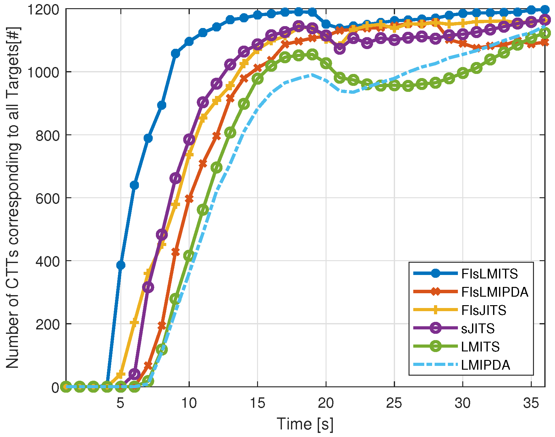
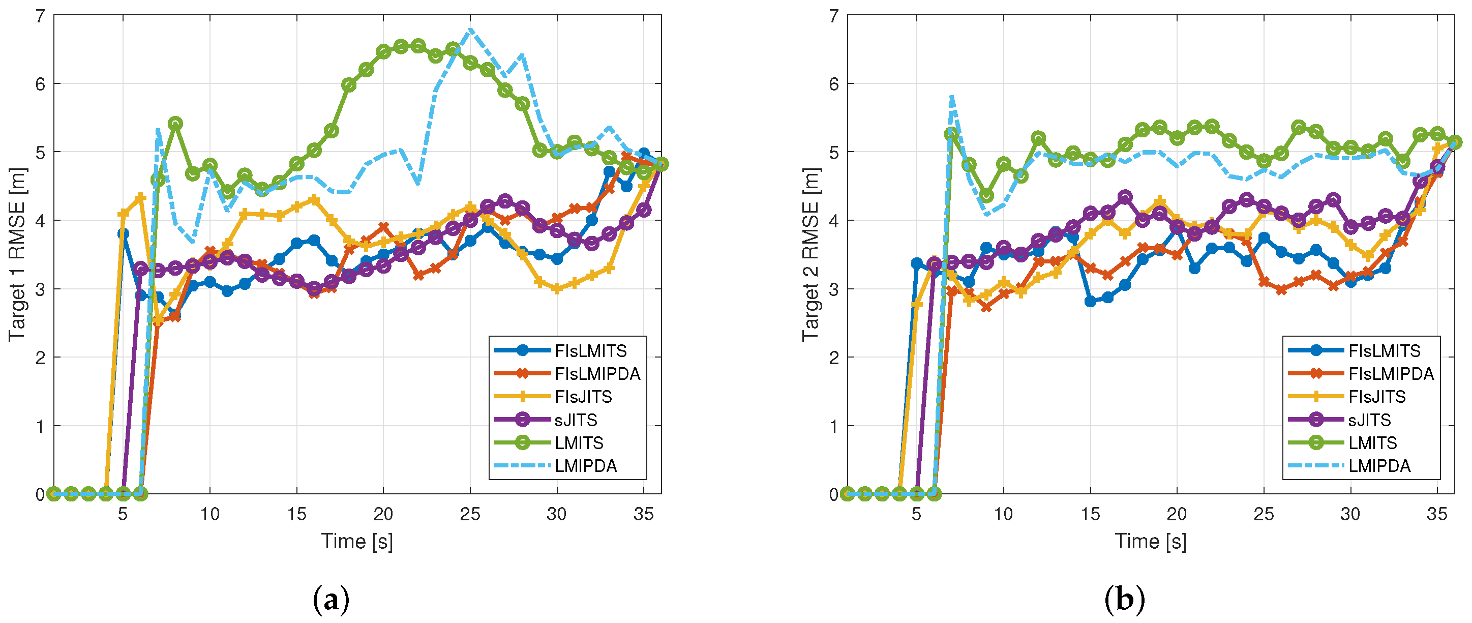
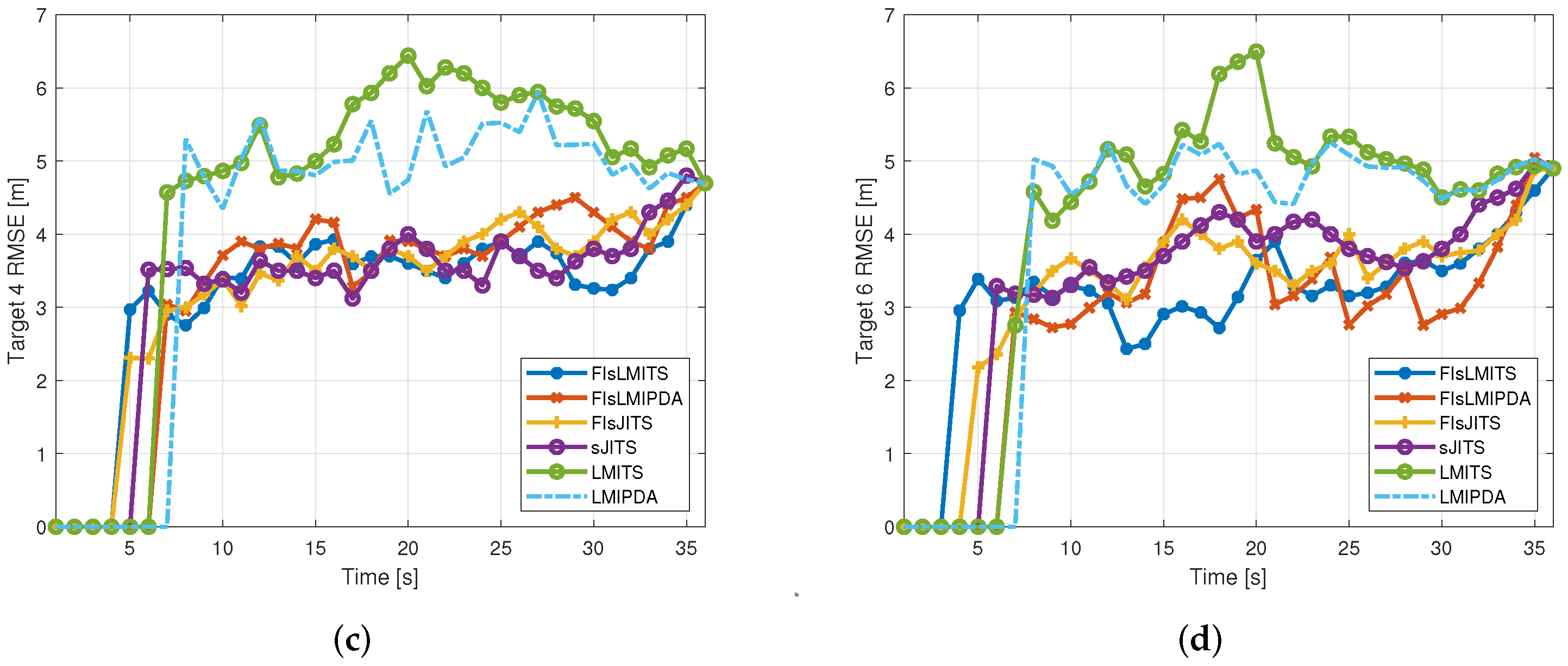
4.3. Illustrative Results

Figure 4 compares the performance of FIsLMITS against the existing algorithms in terms of the number of CTTs corresponding to all targets. The FIsLMITS algorithm confirmed the true track of the potential target quite earlier in scan k = 5 and provided the highest number of CTTs compared to other algorithms. Each smoothing algorithm lost some CTTs near the intersection of multi-targets. However, LMITS and LMIPDA lost the majority of the CTTs in scans k = 20 to 25. It was observed that both FIsJITS and sJITS have almost similar rates of track confirmation. Thus, the proposed FIsLMITS algorithm demonstrates improved estimation accuracy and FTD in comparison to the existing algorithms.
The position root-mean square errors (RMSEs) statistics of the targets with respect to CTTs were calculated using the FIsLMITS, FIsLMIPDA, FIsJITS, sJITS, LMITS, and LMIPDA algorithms for comparison. Since the RMSE trend of the algorithms is almost the same, the RMSE results of only four targets 1, 2, 4, and 6 are shown in Figure 5a, Figure 5b, Figure 5c, and Figure 5d, respectively. LMITS and LMIPDA are non-smoothing algorithms; therefore, they have produced the high estimation errors as compared to smoothing algorithms. The fluctuating RMSE statistics of the FIsJITS and sJITS algorithms corresponding to targets 1, 2, and 6 are observed mainly due to the regular distraction of shared tracks within the vicinity of the neighbored measurements that reflected the highest number of nSwitched (Table 2). In the situation of target 6, FIsLMIPDA, FIsJITS, sJITS, LMITS, and LMIPDA algorithms consistently produced high RMSEs than compared to FIsLMITS algorithms due to the weak growth of smoothing/non-smoothing target existence probabilities in each scan k. In the case of target 4, all smoothing algorithms have almost the same RMSE statistics; however, FIsLMIPDA and sJITS resulted in some peak errors observed at different scans, as depicted in Figure 5c. The FIsLMITS algorithm provides a significant RMSEs reduction compared to the existing algorithms, as shown in Figure 5a–d.
The proposed FIsLMITS algorithm demonstrated the optimum performance in multi-targets cluttered environment in terms of improved state estimation accuracies, track quality measure for FTD, RMSEs, and multi-track retention statisticsm as shown in Figure 3, Figure 4 and Figure 5 and Table 2, respectively.

5. Conclusions

The FIsLMITS extended the LMITS algorithm by utilizing fixed interval smoothing, which significantly improved multi-target state estimation and FTD. In this study, FIsLMITS was implemented for tracking six targets within the 1.67 s execution time per run (each run comprised 36 scans). In view of the simulation setting and algorithm performance, FIsLMITS can feasibly track more than six targets within a bearable execution time. Because the LM-based method avoided the entire joint data association procedure of FIsJITS and sJITS, it saved a huge amount of execution time for multi-target state estimations. To obtain novelty findings, forward track recursion was followed by smoothing multi-tracks estimation. For smoothing, the forward tracks acquired backward multi-tracks predictions that played as a set of measurements in the forward-path track. The fusion of each individual forward track state component with all associated backward multi-track–multi-components consequently calculates the smoothing multi-components and their validation measurements. Each forward track was supported by smoothing multi-component measurements and their component existence probabilities, which significantly improved forward multi-component state estimation, making an efficient forward track for fusion and smoothing in subsequent scans. The Monte Carlo simulation demonstrated the FIsLMITS algorithm to be a useful asset for practical implantation with the highest multi-track retention statistics comprising the highest number of nCases, nOk, and nResult, as well as lowest number of nSwitched and nLost, at the cost of the limited smoothing-time delay.

Author Contributions

S.A.M. has worked for software, methodology, and investigation; I.U. has worked for methodology and writing; U.K. has worked for methodology and editing; T.L.S. has worked as project administration, funding acquisition, and validation of the research. All authors have read and agreed to the published version of the manuscript.

Funding

This work was supported by LIG-Nex1 under the contract LIGNEX1-2021-0966(00).

Institutional Review Board Statement

Not applicable.

Informed Consent Statement

Not applicable.

Data Availability Statement

The research data presented in this study is available on request from the first author.

Acknowledgments

We thank Hanyang University ERICA campus for the provided instruments and laboratory facility for research.

Conflicts of Interest

The authors declare no conflict of interest.

Abbreviations

The following abbreviations are used in this manuscript:
FTDFalse track discrimination
TEPTarget existence probability
MTTMulti-target tracking
STTSingle target tracking
LMLinear multi-target
IPDAIntegrated probabilistic data association
ITSIntegrated track splitting
JIPDAJoint integrated probabilistic data association
JITSJoint integrated track splitting
LMIPDALinear multi-target integrated probabilistic data association
LMITSLinear multi-target integrated track splitting
FIsJIPDAFixed interval smoothing joint integrated probabilistic data association
sJITSSmoothing joint integrated track splitting
FIsJITSFixed interval smoothing joint integrated track splitting
FIsLMIPDAFixed interval smoothing Linear multi-target integrated probabilistic data association
FIsLMITSFixed interval smoothing Linear multi-target integrated track splitting

References

  1. Khaleghi, B.; Khamis, A.; Karray, F.O.; Razavi, S.N. Multisensor data fusion: A review of the state-of-the-art. Inf. Fusion 2013, 14, 28–44. [Google Scholar] [CrossRef]
  2. Challa, S.; Evans, R.; Morelande, M.; Mušicki, D. Fundamentals of Object Tracking; Cambridge University Press: New York, NY, USA, 2011. [Google Scholar]
  3. Mušicki, D.; Evans, R.; Stankovic, S. Integrated probabilistic data association. IEEE Trans. Autom. Control 1994, 39, 1237–1241. [Google Scholar] [CrossRef]
  4. Song, T.L.; Mušicki, D. Target tracking with target state dependent detection. IEEE Trans. Signal Process. 2011, 59, 1063–1074. [Google Scholar] [CrossRef]
  5. Mušicki, D.; Evans, R. JIPDA: Automatic target tracking avoiding track coalescence. IEEE Trans. Aerosp. Electron. Syst. 2015, 51, 962–974. [Google Scholar]
  6. Song, T.L.; Mušicki, D.; Yong, K. Multi-target tracking with state dependent detection. IET Radar Sonar Navig. 2015, 9, 10–18. [Google Scholar] [CrossRef]
  7. Sathyan, T.; Chin, T.; Arulampalam, S.; Suter, D. A Multiple Hypothesis Tracker for Multitarget Tracking with Multiple Simultaneous Measurements. IEEE J. Sel. Top. Signal Process. 2013, 7, 448–460. [Google Scholar] [CrossRef]
  8. Mušicki, D.; Scala, B.L. Multi-target tracking in clutter without measurement assignment. IEEE Trans. Aerosp. Electron. Syst. 2008, 44, 877–896. [Google Scholar] [CrossRef]
  9. Mušicki, D.; Song, T.L.; Lee, H. Linear multitarget finite resolution tracking in clutter. IEEE Trans. Aerosp. Electron. Syst. 2014, 50, 1798–1812. [Google Scholar] [CrossRef]
  10. Bar-Shalom, Y.; Li, X.R.; Kirubarajan, T. Estimation with Applications to Tracking and Navigation: Theory Algorithms and Software; Wiley and Sons, Inc.: New York, NY, USA, 2004. [Google Scholar]
  11. Jason, S.; Travis, B.; Mark, R.; Jason, B.; Moriba, J.; Keric, H. Joint Probabilistic Data Association and Smoothing Applied to Multiple Space Object Tracking. J. Guid. Control. Dyn. 2017, 41, 1–15. [Google Scholar]
  12. Nagappa, S.; Delande, E.D.; Clark, D.E.; Houssineau, J. A Tractable Forward– Backward CPHD Smoother. IEEE Trans. Aeorsp. Electron. Syst. 2017, 53, 201–217. [Google Scholar] [CrossRef]
  13. Koch, W. Fixed-interval retrodiction approach to Bayesian IMM-MHT for maneuvering multiple targets. IEEE Trans. Aerosp. Electron. Syst. 2000, 36, 2–14. [Google Scholar] [CrossRef]
  14. Memon, S.A.; Kim, M.; Shin, M.; Daudpoto, J.; Pathan, D.M.; Son, H. Extended Smoothing Joint Data Association for Multi-target Tracking in Cluttered Environments. IET Radar Sonar Navig. 2020, 14, 564–571. [Google Scholar] [CrossRef]
  15. Memon, S.; Song, T.L.; Kim, T.H. Smoothing Data Association for Target Trajectory Estimation in Cluttered Environments. Eurasip J. Adv. Signal Process. 2016, 21, 1–21. [Google Scholar] [CrossRef] [Green Version]
  16. Memon, S.A.; Song, T.L.; Memon, K.H.; Ullah, I.; Khan, U. Modified Smoothing Data Association for Target Tracking in Clutter. Expert Syst. Appl. 2020, 141, 112969. [Google Scholar] [CrossRef]
  17. Kim, T.H.; Mušicki, D.; Song, T.L.; Lee, C.M. Smoothing joint integrated probabilistic data association. IET Radar Sonar Navig. 2015, 9, 62–66. [Google Scholar] [CrossRef]
  18. Fraser, D.; Potter, J. The optimum linear smoother as a combination of two optimum linear filters. IEEE Trans. Automat. Cont. 1969, 14, 387–390. [Google Scholar] [CrossRef]
  19. Kim, T.H.; Song, T.L. Multi-target multi-scan smoothing in clutter. IET Radar Sonar Navig. 2016, 10, 1270–1276. [Google Scholar] [CrossRef]
  20. Memon, S.A.; Kim, M.; Son, H. Tracking and Estimation of Multiple Cross-over Targets in Clutter. Sensors 2019, 19, 741. [Google Scholar] [CrossRef] [Green Version]
  21. Memon, S.A.; Ullah, I. Detection and tracking of the trajectories of dynamic UAVs in restricted and cluttered environment. Expert Syst. Appl. 2021, 183, 115309. [Google Scholar] [CrossRef]
  22. Memon, S.A.; Kim, W.-G.; Park, M.; Attique, M. Rauch-Tung-Striebel Smoothing Linear Multi-Target Tracking in Clutter. IEEE Access 2021, 10, 3007–3016. [Google Scholar] [CrossRef]
  23. Song, T.L.; Musicki, D. Adaptive clutter measurement density estimation for improved target tracking. IEEE Trans. Aerosp. Electron. Syst. 2011, 47, 1457–1466. [Google Scholar] [CrossRef]
  24. Kim, M.; Memon, S.A.; Shin, M.; Son, H. Dynamic based trajectory estimation and tracking in an uncertain environment. Expert Syst. Appl. 2021, 177, 114919. [Google Scholar] [CrossRef]
  25. Grewal, M.S.; Andrews, A.P. Kalman filtering: Theory and Practice with MATLAB; John Wiley and Sons: New York, NY, USA, 2014. [Google Scholar]
  26. Memon, S.; Son, H.; Memon, A.A.; Ahmed, S. Track Split Smoothing for Target Tracking in Clutter. In Proceedings of the 5th International Conference on Mechanical and Aerospace Engineering (ICASE), Islamabad, Pakistan, 14–16 November 2017. [Google Scholar]
  27. Memon, S.; Son, H.; Memon, K.H.; Ansari, A. Multi-scan smoothing for tracking manoeuvering target trajectory in heavy cluttered environment. IET Radar Sonar Navig. 2017, 11, 1815–1821. [Google Scholar] [CrossRef]
  28. Blackman, S.; Popoli, R. Design and Analysis of Modern Tracking Systems; Artech House: Boston, MA, USA; London, UK, 1999. [Google Scholar]
  29. Salmond, D.J. Mixture Reduction Algorithms for Target Tracking in Clutter. SPIE 1990, 1305, 434–445. [Google Scholar]
  30. Jia, B.; Pham, K.; Blasch, E.; Shen, D.; Chen, G. Consensus-based auction algorithm for distributed sensor management in space object tracking. In Proceedings of the 2017 IEEE Aerospace Conference, Big Sky, MT, USA, 4–11 March 2017. [Google Scholar]
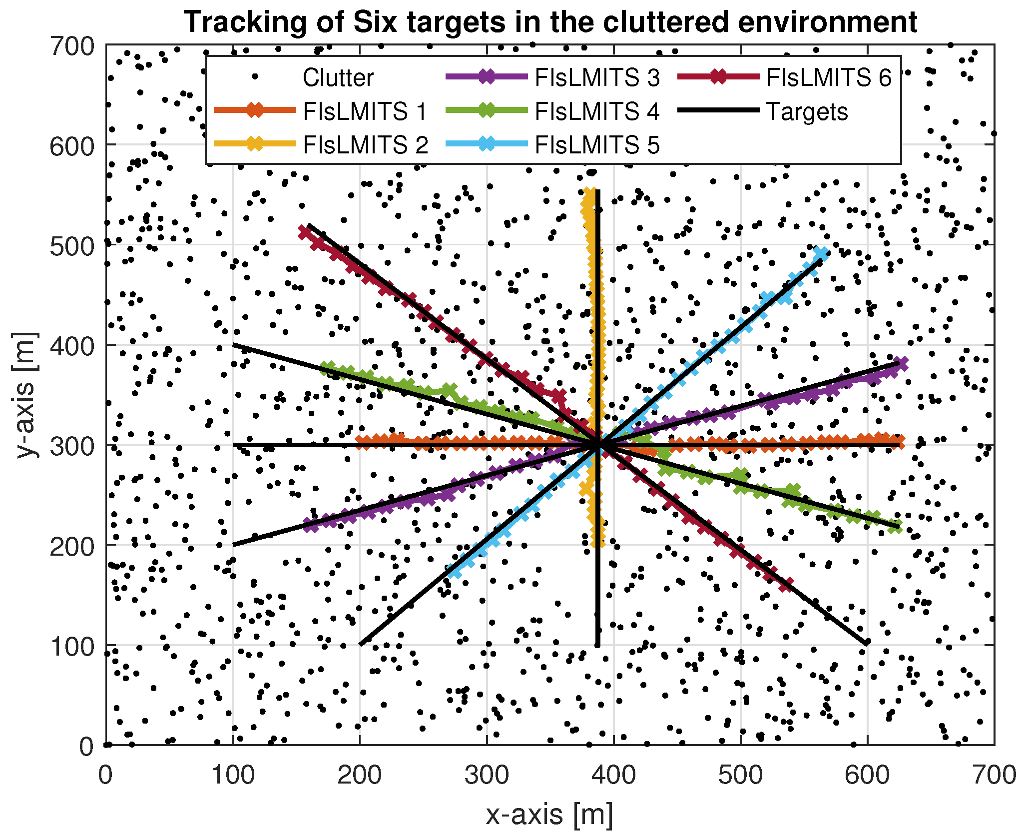
Figure 1. Fixed measurement interval smoothing.
Remotesensing 14 01289 g001
Figure 2. Forward track fusion components associated with backward multi-track components.
Remotesensing 14 01289 g002
Figure 3. Multi-target tracking scenario in the cluttered environment.
Remotesensing 14 01289 g003
Figure 4. Number of CTTs produced by FIsLMITS, FIsLMIPDA, FIsJITS, sJITS, LMITS, and LMIPDA.
Remotesensing 14 01289 g004
Figure 5. Root mean square errors (RMSEs). (a) RMSE of Target 1; (b) RMSE of Target 2; (c) RMSE of Target 4; (d) RMSE of Target 6.
Remotesensing 14 01289 g005aRemotesensing 14 01289 g005b
Table 1. Initial position of targets in meters.
Target No.Position
1[100; 300]
2[387; 100]
3[100; 200]
4[100; 400]
5[200; 100]
6[600; 100]
Table 2. Multi-track retention statistics.
AlgorithmnCasesnOknSwitchednLostnResultExecution Time
FIsLMITS118597819215119711.2
FIsLMIPDA109072026011010945.4
FIsJITS115461149746116316.3
sJITS111964839081116516.8
LMITS99659519720411237.2
LMIPDA105562228814511450.7
Publisher’s Note: MDPI stays neutral with regard to jurisdictional claims in published maps and institutional affiliations.

