
Monitoring the Spatio-Temporal Dynamics of Shale Oil/Gas Development with Landsat Time Series: Case Studies in the USA


Abstract
:1. Introduction
2. Materials and Methods
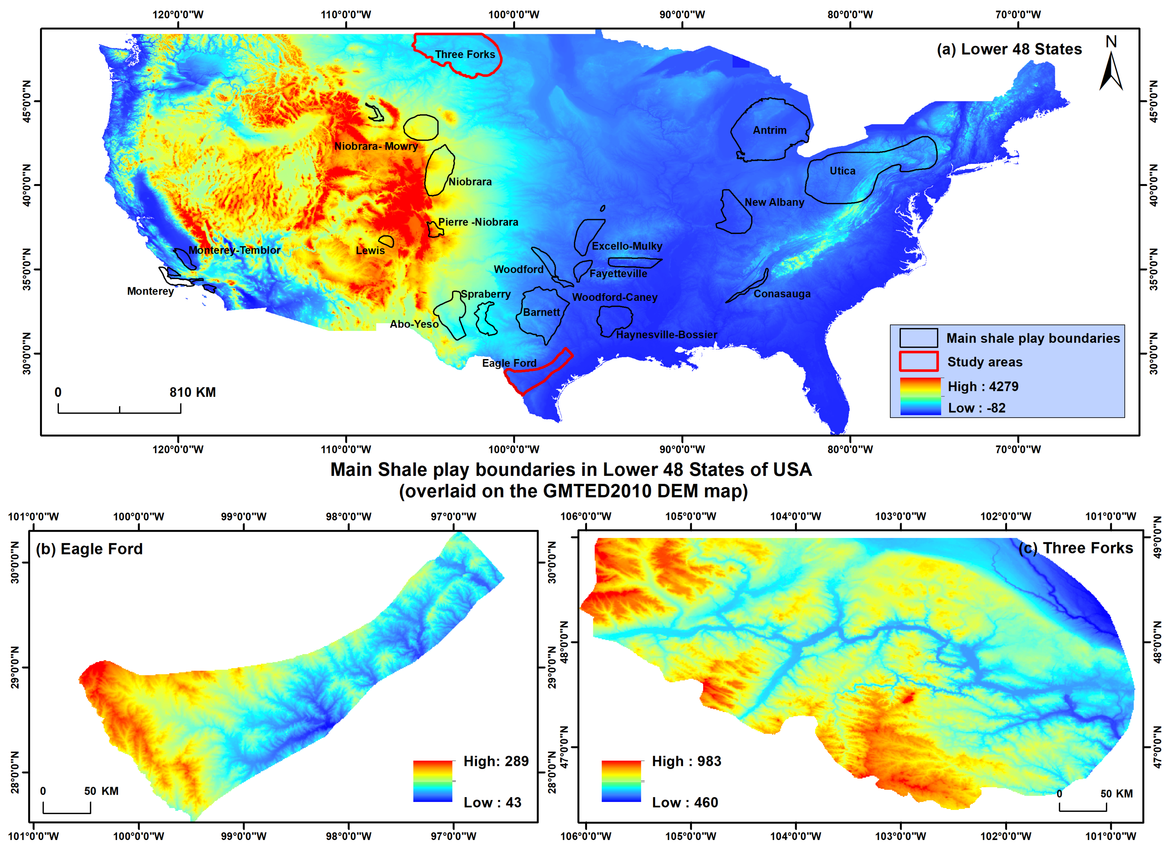
2.1. Study Areas
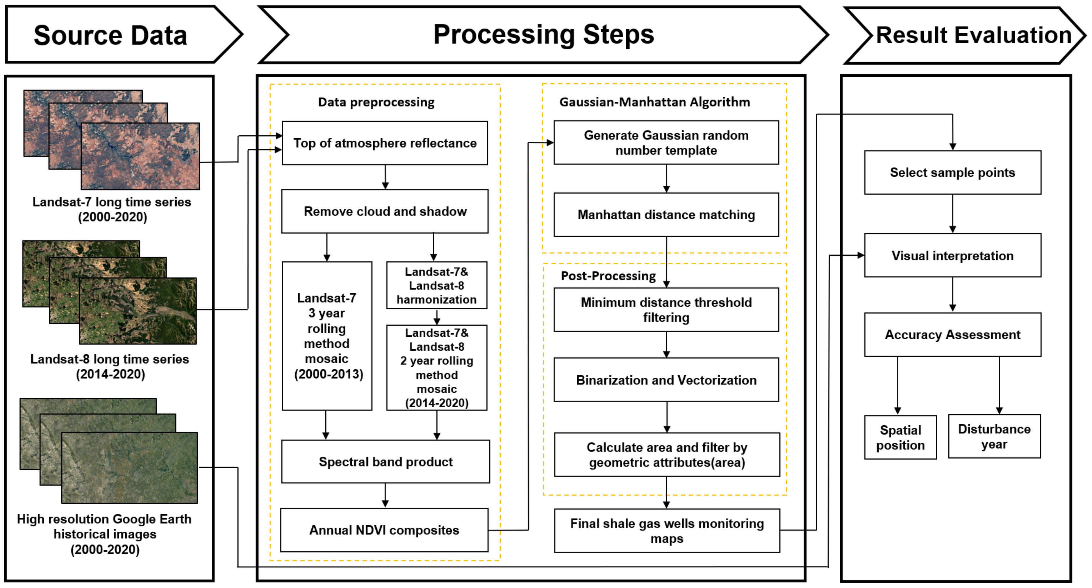
2.2. Workflow
2.3. Data Preprocessing
2.3.1. Data
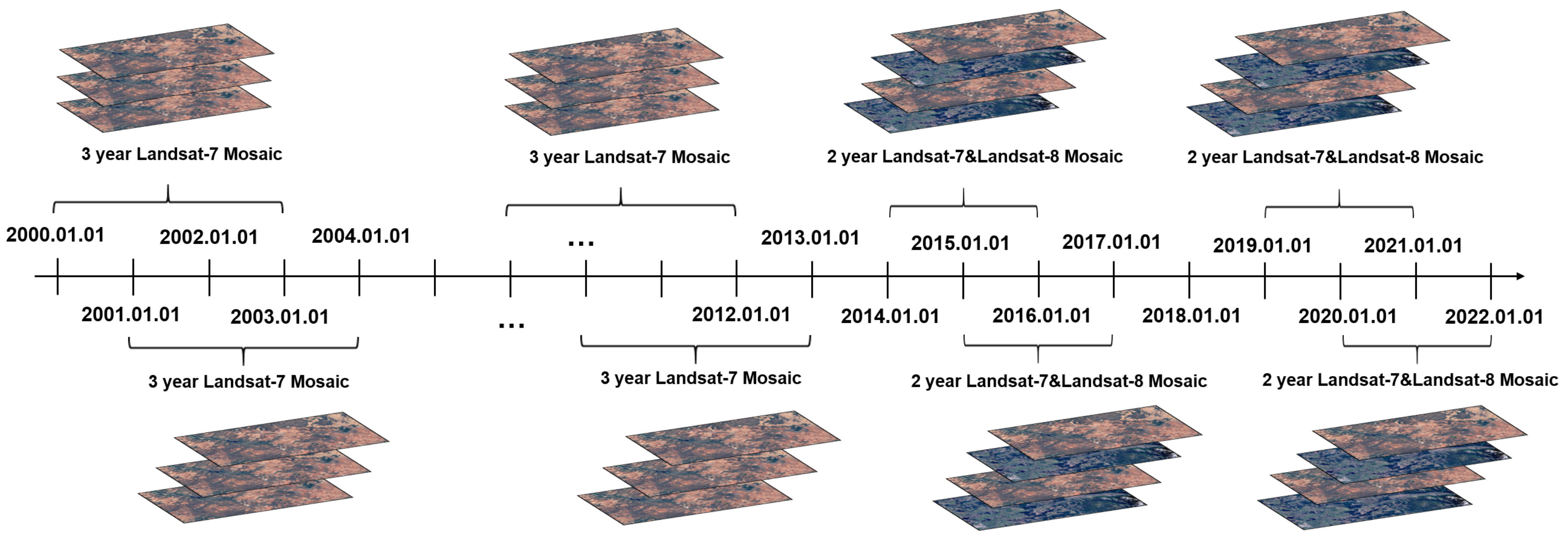
2.3.2. Data Preparation
2.3.3. Annual NDVI Composite
2.4. Shale Oil/Gas Platforms Appearance in Remote Sensing Images
2.5. The Gaussian-Manhattan Models
2.5.1. Simulated NDVI Trajectory Templates
2.5.2. Model Matching with the Minimum Manhattan Distance
2.6. Post-Processing
2.6.1. The Minimum Distance Threshold
2.6.2. Filtering with the Geometric Area Property
3. Results
3.1. Multi-Year Disturbance Detection Map
3.2. Detection Accuracy Analysis
3.2.1. Classification Accuracy
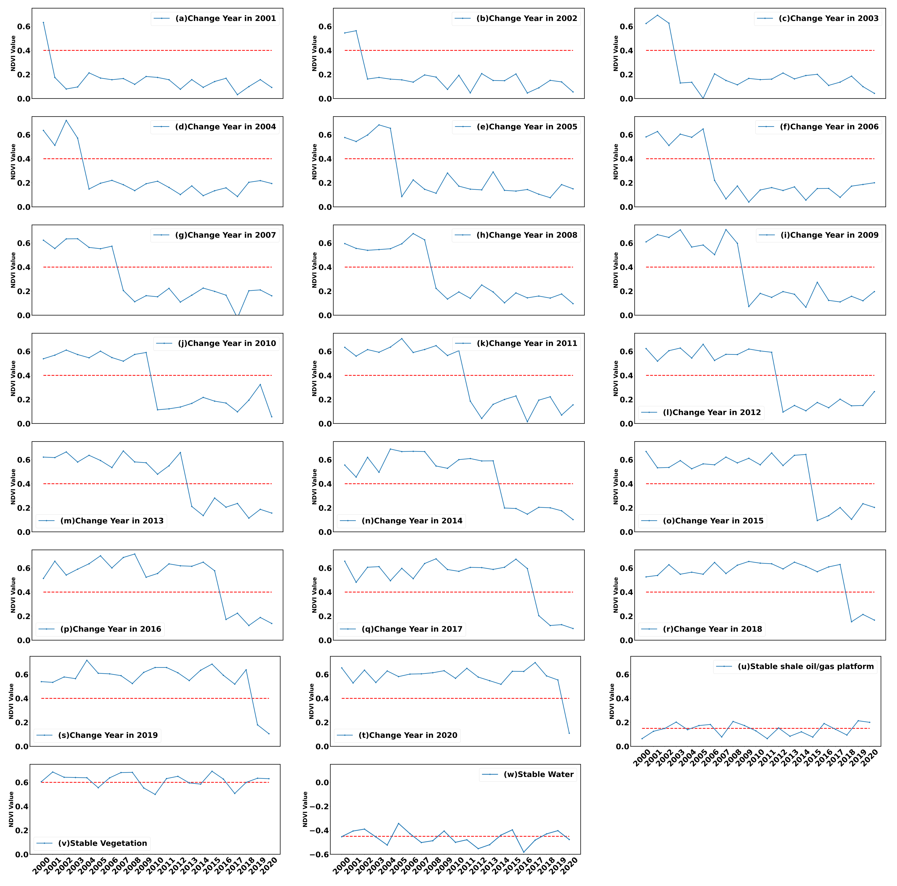
3.2.2. Disturbance Year Accuracy
4. Discussion
4.1. Comparison with Other Algorithms
4.2. Influence of Different Vegetation Growth Conditions
4.3. Limitations of the Shale Oil/Gas Research
5. Conclusions
Author Contributions
Funding
Institutional Review Board Statement
Informed Consent Statement
Data Availability Statement
Conflicts of Interest
References
- Murphy, T. Financial Times. Available online: https://www.ft.com/content/a5292644-958d-4065-92e8-ace55d766654 (accessed on 23 November 2021).
- Duan, H.; Liu, Y. Research on a grey prediction model based on energy prices and its applications. Comput. Ind. Eng. 2021, 162, 107729. [Google Scholar] [CrossRef]
- Hussain, M.; Chen, D.; Cheng, A.; Wei, H.; Stanley, D. Change detection from remotely sensed images: From pixel-based to object-based approaches. ISPRS J. Photogramm. Remote Sens. 2013, 80, 91–106. [Google Scholar] [CrossRef]
- Dean, N. Energy policy: Guiding green lighting. Nat. Energy 2017, 2, 17146. [Google Scholar] [CrossRef]
- Pradhan, R.P.; Arvin, M.B.; Nair, M.; Bennett, S.E.; Hall, J.H. The dynamics between energy consumption patterns, financial sector development and economic growth in Financial Action Task Force (FATF) countries. Energy 2018, 159, 42–53. [Google Scholar] [CrossRef]
- Hu, H.; Lin, J.; Liu, L.; Wu, Y. Cognitive Biases in Understanding the Influence of Shale Gas Exploitation: From Environmental and Economic Perspectives. Front. Energy Res. 2021, 9, 730526. [Google Scholar] [CrossRef]
- Güney, T. Renewable energy consumption and sustainable development in high-income countries. Int. J. Sustain. Dev. World Ecol. 2021, 28, 376–385. [Google Scholar] [CrossRef]
- Alexander, T.; Baihly, J.; Boyer, C.; Clark, B.; Waters, G.; Jochen, V.; Le Calvez, J.; Lewis, R.; Miller, C.K.; Thaeler, J.; et al. Shale gas revolution. Oilfield Rev. 2011, 23, 40–57. [Google Scholar]
- Le, M.T. An assessment of the potential for the development of the shale gas industry in countries outside of North America. Heliyon 2018, 4, e00516. [Google Scholar] [CrossRef] [Green Version]
- Oil, T.R.S. Shale Gas Resources: An Assessment of 137 Shale Formations in 41 Countries Outside the United States; Independent Statistics & Analysis and US Department of Energy: Washington, DC, USA, 2013.
- Jordan, C.; Bateson, L.; Novellino, A. Environmental baseline monitoring for shale-gas development: Insights for monitoring ground motion using InSAR analysis. Sci. Total Environ. 2019, 696, 134075. [Google Scholar] [CrossRef]
- Yifang, B.; Gong, P.; Gini, C. Global land cover mapping using Earth observation satellite data: Recent progresses and challenges. ISPRS J. Photogramm. Remote Sens. 2015, 103, 1–6. [Google Scholar]
- Zhao, Q.; Yu, L.; Li, X.; Peng, D.; Zhang, Y.; Gong, P. Progress and Trends in the Application of Google Earth and Google Earth Engine. Remote Sens. 2021, 13, 3778. [Google Scholar] [CrossRef]
- Dayal, A.M. Environmental concerns of shale gas production. In Shale Gas; Elsevier: Amsterdam, The Netherlands, 2017; pp. 137–144. [Google Scholar]
- Liu, Y. Remote Sensing of Forest Structural Changes Due to the Recent Boom of Unconventional Shale Gas Extraction Activities in Appalachian Ohio. Remote Sens. 2021, 13, 1453. [Google Scholar] [CrossRef]
- Seto, K.C.; Fragkias, M.; Güneralp, B.; Reilly, M.K. A meta-analysis of global urban land expansion. PLoS ONE 2011, 6, e23777. [Google Scholar] [CrossRef]
- Gong, P.; Li, X.; Wang, J.; Bai, Y.; Chen, B.; Hu, T.; Liu, X.; Xu, B.; Yang, J.; Zhang, W.; et al. Annual maps of global artificial impervious area (GAIA) between 1985 and 2018. Remote Sens. Environ. 2020, 236, 111510. [Google Scholar] [CrossRef]
- Liu, X.; Huang, Y.; Xu, X.; Li, X.; Li, X.; Ciais, P.; Lin, P.; Gong, K.; Ziegler, A.D.; Chen, A.; et al. High-spatiotemporal-resolution mapping of global urban change from 1985 to 2015. Nat. Sustain. 2020, 3, 564–570. [Google Scholar] [CrossRef]
- Zhu, Z.; Zhang, J.; Yang, Z.; Aljaddani, A.H.; Cohen, W.B.; Qiu, S.; Zhou, C. Continuous monitoring of land disturbance based on Landsat time series. Remote Sens. Environ. 2020, 238, 111116. [Google Scholar] [CrossRef]
- Xu, H.; Wei, Y.; Liu, C.; Li, X.; Fang, H. A scheme for the long-term monitoring of impervious- relevant land disturbances using high frequency Landsat archives and the Google Earth engine. Remote Sens. 2019, 11, 1891. [Google Scholar] [CrossRef] [Green Version]
- Rodman, K.C.; Andrus, R.A.; Veblen, T.T.; Hart, S.J. Disturbance detection in landsat time series is influenced by tree mortality agent and severity, not by prior disturbance. Remote Sens. Environ. 2021, 254, 112244. [Google Scholar] [CrossRef]
- Wang, B.; Choi, S.; Byun, Y.; Lee, S.; Choi, J. Object-based change detection of very high resolution satellite imagery using the cross-sharpening of multitemporal data. IEEE Geosci. Remote Sens. Lett. 2015, 12, 1151–1155. [Google Scholar] [CrossRef]
- Ilsever, M.; Ünsalan, C. Pixel-based change detection methods. In Two-Dimensional Change Detection Methods; Springer: London, UK, 2012; pp. 7–21. [Google Scholar]
- Gu, W.; Lv, Z.; Hao, M. Change detection method for remote sensing images based on an improved Markov random field. Multimed. Tools Appl. 2017, 76, 17719–17734. [Google Scholar] [CrossRef]
- Ma, W.; Xiong, Y.; Wu, Y.; Yang, H.; Zhang, X.; Jiao, L. Change detection in remote sensing images based on image mapping and a deep capsule network. Remote Sens. 2019, 11, 626. [Google Scholar] [CrossRef] [Green Version]
- Ferraris, V.; Dobigeon, N.; Wei, Q.; Chabert, M. Detecting changes between optical images of different spatial and spectral resolutions: A fusion-based approach. IEEE Trans. Geosci. Remote Sens. 2017, 56, 1566–1578. [Google Scholar] [CrossRef]
- Dwyer, J.; Sayler, K.; Zylstra, G. Landsat pathfinder data sets for landscape change analysis. In Proceedings of the IGARSS’96: 1996 International Geoscience and Remote Sensing Symposium, Lincoln, NE, USA, 31–31 May 1996; Volume 1, pp. 547–550. [Google Scholar]
- Byun, Y.; Han, D. Relative radiometric normalization of bitemporal very high-resolution satellite images for flood change detection. J. Appl. Remote Sens. 2018, 12, 026021. [Google Scholar] [CrossRef]
- Gandhi, G.M.; Parthiban, S.; Thummalu, N.; Christy, A. Ndvi: Vegetation change detection using remote sensing and gis—A case study of Vellore District. Procedia Comput. Sci. 2015, 57, 1199–1210. [Google Scholar] [CrossRef] [Green Version]
- Xu, R.; Liu, J.; Xu, J. Extraction of high-precision urban impervious surfaces from sentinel-2 multispectral imagery via modified linear spectral mixture analysis. Sensors 2018, 18, 2873. [Google Scholar] [CrossRef] [Green Version]
- Qi, Z.; Yeh, A.G.O.; Li, X.; Zhang, X. A three-component method for timely detection of land cover changes using polarimetric SAR images. ISPRS J. Photogramm. Remote Sens. 2015, 107, 3–21. [Google Scholar] [CrossRef]
- Asokan, A.; Anitha, J. Change detection techniques for remote sensing applications: A survey. Earth Sci. Inform. 2019, 12, 143–160. [Google Scholar] [CrossRef]
- Deng, J.; Wang, K.; Deng, Y.; Qi, G. PCA-based land-use change detection and analysis using multitemporal and multisensor satellite data. Int. J. Remote Sens. 2008, 29, 4823–4838. [Google Scholar] [CrossRef]
- You, Y.; Cao, J.; Zhou, W. A survey of change detection methods based on remote sensing images for multi-source and multi-objective scenarios. Remote Sens. 2020, 12, 2460. [Google Scholar] [CrossRef]
- Kyere, I.; Astor, T.; Graß, R.; Wachendorf, M. Multi-temporal agricultural land-Cover mapping using single-year and multi-year models based on Landsat imagery and IACS data. Agronomy 2019, 9, 309. [Google Scholar] [CrossRef] [Green Version]
- Im, J.; Jensen, J.R. A change detection model based on neighborhood correlation image analysis and decision tree classification. Remote Sens. Environ. 2005, 99, 326–340. [Google Scholar] [CrossRef]
- Xing, J.; Sieber, R.; Caelli, T. A scale-invariant change detection method for land use/cover change research. ISPRS J. Photogramm. Remote Sens. 2018, 141, 252–264. [Google Scholar] [CrossRef]
- Liu, D.; Qi, Z.; Zhang, H.; Li, X.; Yeh, A.G.O.; Wang, J. Investigation of the capability of multitemporal RADARSAT-2 fully polarimetric SAR images for land cover classification: A case of Panyu, Guangdong province. Eur. J. Remote Sens. 2021, 54, 338–350. [Google Scholar] [CrossRef]
- Mou, L.; Bruzzone, L.; Zhu, X.X. Learning spectral-spatial-temporal features via a recurrent convolutional neural network for change detection in multispectral imagery. IEEE Trans. Geosci. Remote Sens. 2018, 57, 924–935. [Google Scholar] [CrossRef] [Green Version]
- Kong, Y.L.; Huang, Q.; Wang, C.; Chen, J.; Chen, J.; He, D. Long short-term memory neural networks for online disturbance detection in satellite image time series. Remote Sens. 2018, 10, 452. [Google Scholar] [CrossRef] [Green Version]
- Tan, X.; Li, M.; Zhang, P.; Wu, Y.; Jiao, M. Multispectral image change detection with kernel cross-modal factor analysis-based fusion of kernels. J. Appl. Remote Sens. 2018, 12, 035008. [Google Scholar]
- Blaschke, T. Object based image analysis for remote sensing. ISPRS J. Photogramm. Remote Sens. 2010, 65, 2–16. [Google Scholar] [CrossRef] [Green Version]
- Hossain, M.D.; Chen, D. Segmentation for Object-Based Image Analysis (OBIA): A review of algorithms and challenges from remote sensing perspective. ISPRS J. Photogramm. Remote Sens. 2019, 150, 115–134. [Google Scholar] [CrossRef]
- Verbesselt, J.; Hyndman, R.; Newnham, G.; Culvenor, D. Detecting trend and seasonal changes in satellite image time series. Remote Sens. Environ. 2010, 114, 106–115. [Google Scholar] [CrossRef]
- Kennedy, R.E.; Yang, Z.; Cohen, W.B. Detecting trends in forest disturbance and recovery using yearly Landsat time series: 1. LandTrendr—Temporal segmentation algorithms. Remote Sens. Environ. 2010, 114, 2897–2910. [Google Scholar] [CrossRef]
- Bradley, B.A.; Jacob, R.W.; Hermance, J.F.; Mustard, J.F. A curve fitting procedure to derive inter-annual phenologies from time series of noisy satellite NDVI data. Remote Sens. Environ. 2007, 106, 137–145. [Google Scholar] [CrossRef]
- White, M.A.; Nemani, R.R. Real-time monitoring and short-term forecasting of land surface phenology. Remote Sens. Environ. 2006, 104, 43–49. [Google Scholar] [CrossRef]
- Bontemps, S.; Bogaert, P.; Titeux, N.; Defourny, P. An object-based change detection method accounting for temporal dependences in time series with medium to coarse spatial resolution. Remote Sens. Environ. 2008, 112, 3181–3191. [Google Scholar] [CrossRef]
- Fensholt, R.; Rasmussen, K.; Nielsen, T.T.; Mbow, C. Evaluation of earth observation based long term vegetation trends—Intercomparing NDVI time series trend analysis consistency of Sahel from AVHRR GIMMS, Terra MODIS and SPOT VGT data. Remote Sens. Environ. 2009, 113, 1886–1898. [Google Scholar] [CrossRef]
- Arévalo, P.; Olofsson, P.; Woodcock, C.E. Continuous monitoring of land change activities and post-disturbance dynamics from Landsat time series: A test methodology for REDD+ reporting. Remote Sens. Environ. 2020, 238, 111051. [Google Scholar] [CrossRef]
- Kennedy, R.E.; Yang, Z.; Gorelick, N.; Braaten, J.; Cavalcante, L.; Cohen, W.B.; Healey, S. Implementation of the LandTrendr algorithm on google earth engine. Remote Sens. 2018, 10, 691. [Google Scholar] [CrossRef] [Green Version]
- Xiao, W.; Deng, X.; He, T.; Chen, W. Mapping annual land disturbance and reclamation in a surface coal mining region using google earth engine and the landtrendr algorithm: A case study of the shengli coalfield in Inner Mongolia, China. Remote Sens. 2020, 12, 1612. [Google Scholar] [CrossRef]
- Xue, J.; Su, B. Significant remote sensing vegetation indices: A review of developments and applications. J. Sens. 2017, 2017, 1353691. [Google Scholar] [CrossRef] [Green Version]
- Wu, Q.; Jin, Y.; Fan, H. Evaluating and comparing performances of topographic correction methods based on multi-source DEMs and Landsat-8 OLI data. Int. J. Remote Sens. 2016, 37, 4712–4730. [Google Scholar] [CrossRef]
- United Nations Conference on Trade and Development (UNCTAD). Commodities at A Glance: Special Issue on Shale Gas. In Proceedings of the United Nations Conference on Trade and Development, New York, NY, USA, 23–26 April 2018.
- Budge, K.G. Shale Gas. Available online: https://en.wikipedia.org/wiki/Shale_gas (accessed on 15 December 2021).
- EIA. Main Shale Plays. Available online: https://www.eia.gov/maps/images/shale_gas_lower48.pdf (accessed on 1 January 2022).
- Speight, J.G. Shale Oil and Gas Production Processes; Gulf Professional Publishing: Amsterdam, The Netherlands, 2019. [Google Scholar]
- AACOG Natural Resources Department. Oil and Gas Emission Inventory, Eagle Ford Shale. San Antonio: Alamo Area Council of Governments: 260. 2014. Available online: http://www.aacog.com/documentcenter/view/19069 (accessed on 1 January 2022).
- Berwick, B.R.; Hendricks, M.L. Depositional lithofacies of the Upper Devonian Three Forks Formation and the Grassy Butte Member of the Lower Bakken Shale in the Williston Basin. In The Bakken–Three Forks Petroleum System in the Williston Basin; Robinson, J.W., LeFever, J.A., Gaswirth, S.B., Eds.; Rocky Mountain Association of Geologists: Denver, CO, USA, 2011; pp. 159–172. [Google Scholar]
- Gaswirth, S.B.; Marra, K.R. US Geological Survey 2013 assessment of undiscovered resources in the Bakken and Three Forks Formations of the US Williston Basin Province. AAPG Bull. 2015, 99, 639–660. [Google Scholar] [CrossRef]
- Markham, B.L.; Storey, J.C.; Williams, D.L.; Irons, J.R. Landsat sensor performance: History and current status. IEEE Trans. Geosci. Remote Sens. 2004, 42, 2691–2694. [Google Scholar] [CrossRef]
- Liu, Y.; Hu, C.; Sun, C.; Zhan, W.; Sun, S.; Xu, B.; Dong, Y. Assessment of offshore oil/gas platform status in the northern Gulf of Mexico using multi-source satellite time-series images. Remote Sens. Environ. 2018, 208, 63–81. [Google Scholar] [CrossRef]
- Morel, A.C.; Fisher, J.B.; Malhi, Y. Evaluating the potential to monitor aboveground biomass in forest and oil palm in Sabah, Malaysia, for 2000–2008 with Landsat ETM+ and ALOS-PALSAR. Int. J. Remote Sens. 2012, 33, 3614–3639. [Google Scholar] [CrossRef]
- Nooni, I.; Duker, A.; Van Duren, I.; Addae-Wireko, L.; Osei Jnr, E. Support vector machine to map oil palm in a heterogeneous environment. Int. J. Remote Sens. 2014, 35, 4778–4794. [Google Scholar] [CrossRef]
- USGS. What Are the Band Designations for the Landsat Satellites? Available online: https://www.usgs.gov/faqs/what-are-band-designations-landsat-satellites (accessed on 28 December 2021).
- Gorelick, N.; Hancher, M.; Dixon, M.; Ilyushchenko, S.; Thau, D.; Moore, R. Google Earth Engine: Planetary-scale geospatial analysis for everyone. Remote Sens. Environ. 2017, 202, 18–27. [Google Scholar] [CrossRef]
- Chander, G.; Markham, B.L.; Helder, D.L. Summary of current radiometric calibration coefficients for Landsat MSS, TM, ETM+, and EO-1 ALI sensors. Remote Sens. Environ. 2009, 113, 893–903. [Google Scholar] [CrossRef]
- Developers, G. Landsat Algorithms. Available online: https://developers.google.com/earth-engine/guides/landsat#landsat-collection-structure (accessed on 30 December 2021).
- USGS. Landsat Collection 1 Level-1 Quality Assessment Band. Available online: https://www.usgs.gov/landsat-missions/landsat-collection-1-level-1-quality-assessment-band (accessed on 30 December 2021).
- Zhang, Q.; Li, B.; Thau, D.; Moore, R. Building a better urban picture: Combining day and night remote sensing imagery. Remote Sens. 2015, 7, 11887–11913. [Google Scholar] [CrossRef] [Green Version]
- Roy, D.P.; Kovalskyy, V.; Zhang, H.; Vermote, E.F.; Yan, L.; Kumar, S.; Egorov, A. Characterization of Landsat-7 to Landsat-8 reflective wavelength and normalized difference vegetation index continuity. Remote Sens. Environ. 2016, 185, 57–70. [Google Scholar] [CrossRef] [Green Version]
- Runge, A.; Grosse, G. Mosaicking Landsat and Sentinel-2 Data to Enhance LandTrendr Time Series Analysis in Northern High Latitude Permafrost Regions. Remote Sens. 2020, 12, 2471. [Google Scholar] [CrossRef]
- Zuckerkandl, E.; Pauling, L. Evolutionary divergence and convergence in proteins. In Evolving Genes and Proteins; Elsevier: New York, NY, USA, 1965; pp. 97–166. [Google Scholar]
- Oreopoulos, L.; Wilson, M.J.; Várnai, T. Implementation on Landsat data of a simple cloud-mask algorithm developed for MODIS land bands. IEEE Geosci. Remote Sens. Lett. 2011, 8, 597–601. [Google Scholar] [CrossRef] [Green Version]
- Qiu, S.; He, B.; Zhu, Z.; Liao, Z.; Quan, X. Improving Fmask cloud and cloud shadow detection in mountainous area for Landsats 4–8 images. Remote Sens. Environ. 2017, 199, 107–119. [Google Scholar] [CrossRef]
- Yu, L.; Ball, S.B.; Blinn, C.E.; Moeltner, K.; Peery, S.; Thomas, V.A.; Wynne, R.H. Cloud-Sourcing: Using an online labor force to detect clouds and cloud shadows in Landsat images. Remote Sens. 2015, 7, 2334–2351. [Google Scholar] [CrossRef] [Green Version]
- Chai, D.; Newsam, S.; Zhang, H.K.; Qiu, Y.; Huang, J. Cloud and cloud shadow detection in Landsat imagery based on deep convolutional neural networks. Remote Sens. Environ. 2019, 225, 307–316. [Google Scholar] [CrossRef]
- Chen, Y.; He, W.; Yokoya, N.; Huang, T.Z. Blind cloud and cloud shadow removal of multitemporal images based on total variation regularized low-rank sparsity decomposition. ISPRS J. Photogramm. Remote Sens. 2019, 157, 93–107. [Google Scholar] [CrossRef]
- Goodwin, N.R.; Collett, L.J.; Denham, R.J.; Flood, N.; Tindall, D. Cloud and cloud shadow screening across Queensland, Australia: An automated method for Landsat TM/ETM+ time series. Remote Sens. Environ. 2013, 134, 50–65. [Google Scholar] [CrossRef]
- Jin, S.; Homer, C.; Yang, L.; Xian, G.; Fry, J.; Danielson, P.; Townsend, P.A. Automated cloud and shadow detection and filling using two-date Landsat imagery in the USA. Int. J. Remote Sens. 2013, 34, 1540–1560. [Google Scholar] [CrossRef]
- Holben, B.N. Characteristics of maximum-value composite images from temporal AVHRR data. Int. J. Remote Sens. 1986, 7, 1417–1434. [Google Scholar] [CrossRef]
- Julien, Y.; Sobrino, J.A. Comparison of cloud-reconstruction methods for time series of composite NDVI data. Remote Sens. Environ. 2010, 114, 618–625. [Google Scholar] [CrossRef]
- Capoccia, C. Minimum Distance Method. Available online: https://en.wikipedia.org/wiki/Minimum-distance_estimation (accessed on 28 December 2021).
- Xu, Y.; Yu, L.; Peng, D.; Zhao, J.; Cheng, Y.; Liu, X.; Li, W.; Meng, R.; Xu, X.; Gong, P. Annual 30-m land use/land cover maps of China for 1980–2015 from the integration of AVHRR, MODIS and Landsat data using the BFAST algorithm. Sci. China Earth Sci. 2020, 63, 1390–1407. [Google Scholar] [CrossRef]
- Dara, A.; Baumann, M.; Kuemmerle, T.; Pflugmacher, D.; Rabe, A.; Griffiths, P.; Hölzel, N.; Kamp, J.; Freitag, M.; Hostert, P. Mapping the timing of cropland abandonment and recultivation in northern Kazakhstan using annual Landsat time series. Remote Sens. Environ. 2018, 213, 49–60. [Google Scholar] [CrossRef]


| Data Set | Data Name | Spatial Resolution | Date | Source |
|---|---|---|---|---|
| Landsat | Landsat-7/ETM+ | 30 m | 11 January 2000–16 November 2021 | GEE 1 |
| Landsat-8/OLI | 30 m | 15 January 2014–10 December 2021 | GEE | |
| High-resolution data | DigitalGlobe Imagery | / | 2000–2020 | Google Earth |
| Area Interval (m2) | Right Points | False Points | Total Points | Accuracy |
|---|---|---|---|---|
| (0, 3000] | 3 | 97 | 100 | 3% |
| (3000, 30,000] | 94 | 6 | 100 | 94% |
| (30,000, 60,000] | 91 | 9 | 100 | 91% |
| (60,000, 125,426] | 11 | 89 | 100 | 89% |
| Right Vector Spots | False Vector Spots | Total Vector Spots | Accuracy | |
|---|---|---|---|---|
| Eagle Ford | 419 | 81 | 500 | 83.80% |
| Three Forks | 407 | 95 | 500 | 81.40% |
| Year | 2001 | 2002 | 2003 | 2004 | 2005 | 2006 | 2007 | 2008 | 2009 | 2010 | 2011 | 2012 | 2013 | 2014 | 2015 | 2016 | 2017 | 2018 | 2019 | 2020 |
|---|---|---|---|---|---|---|---|---|---|---|---|---|---|---|---|---|---|---|---|---|
| 2000 | 2 | 0 | 0 | 0 | 0 | 0 | 0 | 0 | 0 | 0 | 0 | 0 | 0 | 0 | 0 | 0 | 0 | 0 | 0 | 0 |
| 2001 | 20 | 2 | 0 | 0 | 0 | 0 | 0 | 0 | 0 | 0 | 0 | 0 | 0 | 0 | 0 | 0 | 0 | 0 | 0 | 0 |
| 2002 | 5 | 22 | 3 | 0 | 0 | 0 | 0 | 0 | 0 | 0 | 0 | 0 | 0 | 0 | 0 | 0 | 0 | 0 | 0 | 0 |
| 2003 | 3 | 3 | 26 | 1 | 0 | 0 | 0 | 0 | 0 | 0 | 0 | 0 | 0 | 0 | 0 | 0 | 0 | 0 | 0 | 0 |
| 2004 | 0 | 3 | 1 | 21 | 1 | 0 | 0 | 0 | 0 | 0 | 0 | 0 | 0 | 0 | 0 | 0 | 0 | 0 | 0 | 0 |
| 2005 | 0 | 0 | 0 | 6 | 24 | 3 | 0 | 0 | 0 | 0 | 0 | 0 | 0 | 0 | 0 | 0 | 0 | 0 | 0 | 0 |
| 2006 | 0 | 0 | 0 | 2 | 3 | 22 | 1 | 0 | 0 | 0 | 0 | 0 | 0 | 0 | 0 | 0 | 0 | 0 | 0 | 0 |
| 2007 | 0 | 0 | 0 | 0 | 2 | 4 | 26 | 2 | 0 | 0 | 0 | 0 | 0 | 0 | 0 | 0 | 0 | 0 | 0 | 0 |
| 2008 | 0 | 0 | 0 | 0 | 0 | 1 | 1 | 26 | 3 | 0 | 0 | 0 | 0 | 0 | 0 | 0 | 0 | 0 | 0 | 0 |
| 2009 | 0 | 0 | 0 | 0 | 0 | 0 | 2 | 2 | 23 | 2 | 0 | 0 | 0 | 0 | 0 | 0 | 0 | 0 | 0 | 0 |
| 2010 | 0 | 0 | 0 | 0 | 0 | 0 | 0 | 0 | 4 | 25 | 2 | 0 | 0 | 0 | 0 | 0 | 0 | 0 | 0 | 0 |
| 2011 | 0 | 0 | 0 | 0 | 0 | 0 | 0 | 0 | 0 | 3 | 27 | 1 | 0 | 0 | 0 | 0 | 0 | 0 | 0 | 0 |
| 2012 | 0 | 0 | 0 | 0 | 0 | 0 | 0 | 0 | 0 | 0 | 1 | 22 | 2 | 0 | 0 | 0 | 0 | 0 | 0 | 0 |
| 2013 | 0 | 0 | 0 | 0 | 0 | 0 | 0 | 0 | 0 | 0 | 0 | 3 | 24 | 1 | 0 | 0 | 0 | 0 | 0 | 0 |
| 2014 | 0 | 0 | 0 | 0 | 0 | 0 | 0 | 0 | 0 | 0 | 0 | 4 | 4 | 26 | 0 | 0 | 0 | 0 | 0 | 0 |
| 2015 | 0 | 0 | 0 | 0 | 0 | 0 | 0 | 0 | 0 | 0 | 0 | 0 | 0 | 3 | 25 | 3 | 0 | 0 | 0 | 0 |
| 2016 | 0 | 0 | 0 | 0 | 0 | 0 | 0 | 0 | 0 | 0 | 0 | 0 | 0 | 0 | 3 | 23 | 3 | 0 | 0 | 0 |
| 2017 | 0 | 0 | 0 | 0 | 0 | 0 | 0 | 0 | 0 | 0 | 0 | 0 | 0 | 0 | 2 | 4 | 25 | 3 | 0 | 0 |
| 2018 | 0 | 0 | 0 | 0 | 0 | 0 | 0 | 0 | 0 | 0 | 0 | 0 | 0 | 0 | 0 | 0 | 2 | 26 | 2 | 0 |
| 2019 | 0 | 0 | 0 | 0 | 0 | 0 | 0 | 0 | 0 | 0 | 0 | 0 | 0 | 0 | 0 | 0 | 0 | 1 | 27 | 1 |
| 2020 | 0 | 0 | 0 | 0 | 0 | 0 | 0 | 0 | 0 | 0 | 0 | 0 | 0 | 0 | 0 | 0 | 0 | 0 | 1 | 26 |
| 2021 | 0 | 0 | 0 | 0 | 0 | 0 | 0 | 0 | 0 | 0 | 0 | 0 | 0 | 0 | 0 | 0 | 0 | 0 | 0 | 3 |
| Total | 30 | 30 | 30 | 30 | 30 | 30 | 30 | 30 | 30 | 30 | 30 | 30 | 30 | 30 | 30 | 30 | 30 | 30 | 30 | 30 |
| PA 1 | 66.67 | 73.33 | 86.67 | 70.00 | 80.00 | 73.33 | 86.67 | 86.67 | 76.67 | 83.33 | 90.00 | 73.33 | 80.00 | 86.67 | 83.33 | 76.67 | 83.33 | 86.67 | 90.00 | 86.67 |
| PA[−1] | 73.33 | 80.00 | 96.67 | 73.33 | 83.33 | 83.33 | 90.00 | 93.33 | 86.67 | 90.00 | 96.67 | 76.67 | 86.67 | 90.00 | 83.33 | 86.67 | 93.33 | 96.67 | 90.00 | 90.00 |
| PA[+1] | 83.33 | 83.33 | 90.00 | 90.00 | 90.00 | 86.67 | 90.00 | 93.33 | 90.00 | 93.33 | 93.33 | 83.33 | 93.33 | 96.67 | 93.33 | 90.00 | 90.00 | 90.00 | 93.33 | 96.67 |
| Year | 2001 | 2002 | 2003 | 2004 | 2005 | 2006 | 2007 | 2008 | 2009 | 2010 | 2011 | 2012 | 2013 | 2014 | 2015 | 2016 | 2017 | 2018 | 2019 | 2020 |
|---|---|---|---|---|---|---|---|---|---|---|---|---|---|---|---|---|---|---|---|---|
| 2000 | 1 | 0 | 0 | 0 | 0 | 0 | 0 | 0 | 0 | 0 | 0 | 0 | 0 | 0 | 0 | 0 | 0 | 0 | 0 | 0 |
| 2001 | 21 | 3 | 0 | 0 | 0 | 0 | 0 | 0 | 0 | 0 | 0 | 0 | 0 | 0 | 0 | 0 | 0 | 0 | 0 | 0 |
| 2002 | 5 | 19 | 2 | 0 | 0 | 0 | 0 | 0 | 0 | 0 | 0 | 0 | 0 | 0 | 0 | 0 | 0 | 0 | 0 | 0 |
| 2003 | 3 | 5 | 23 | 1 | 0 | 0 | 0 | 0 | 0 | 0 | 0 | 0 | 0 | 0 | 0 | 0 | 0 | 0 | 0 | 0 |
| 2004 | 0 | 3 | 1 | 25 | 4 | 0 | 0 | 0 | 0 | 0 | 0 | 0 | 0 | 0 | 0 | 0 | 0 | 0 | 0 | 0 |
| 2005 | 0 | 0 | 4 | 2 | 20 | 3 | 0 | 0 | 0 | 0 | 0 | 0 | 0 | 0 | 0 | 0 | 0 | 0 | 0 | 0 |
| 2006 | 0 | 0 | 0 | 2 | 5 | 22 | 2 | 0 | 0 | 0 | 0 | 0 | 0 | 0 | 0 | 0 | 0 | 0 | 0 | 0 |
| 2007 | 0 | 0 | 0 | 0 | 1 | 5 | 24 | 1 | 0 | 0 | 0 | 0 | 0 | 0 | 0 | 0 | 0 | 0 | 0 | 0 |
| 2008 | 0 | 0 | 0 | 0 | 0 | 0 | 3 | 25 | 4 | 0 | 0 | 0 | 0 | 0 | 0 | 0 | 0 | 0 | 0 | 0 |
| 2009 | 0 | 0 | 0 | 0 | 0 | 0 | 1 | 4 | 21 | 2 | 0 | 0 | 0 | 0 | 0 | 0 | 0 | 0 | 0 | 0 |
| 2010 | 0 | 0 | 0 | 0 | 0 | 0 | 0 | 0 | 4 | 26 | 3 | 0 | 0 | 0 | 0 | 0 | 0 | 0 | 0 | 0 |
| 2011 | 0 | 0 | 0 | 0 | 0 | 0 | 0 | 0 | 1 | 2 | 22 | 4 | 0 | 0 | 0 | 0 | 0 | 0 | 0 | 0 |
| 2012 | 0 | 0 | 0 | 0 | 0 | 0 | 0 | 0 | 0 | 0 | 4 | 21 | 2 | 0 | 0 | 0 | 0 | 0 | 0 | 0 |
| 2013 | 0 | 0 | 0 | 0 | 0 | 0 | 0 | 0 | 0 | 0 | 1 | 2 | 25 | 1 | 0 | 0 | 0 | 0 | 0 | 0 |
| 2014 | 0 | 0 | 0 | 0 | 0 | 0 | 0 | 0 | 0 | 0 | 0 | 3 | 2 | 27 | 1 | 0 | 0 | 0 | 0 | 0 |
| 2015 | 0 | 0 | 0 | 0 | 0 | 0 | 0 | 0 | 0 | 0 | 0 | 0 | 1 | 1 | 26 | 2 | 0 | 0 | 0 | 0 |
| 2016 | 0 | 0 | 0 | 0 | 0 | 0 | 0 | 0 | 0 | 0 | 0 | 0 | 0 | 1 | 3 | 24 | 2 | 0 | 0 | 0 |
| 2017 | 0 | 0 | 0 | 0 | 0 | 0 | 0 | 0 | 0 | 0 | 0 | 0 | 0 | 0 | 0 | 4 | 25 | 3 | 0 | 0 |
| 2018 | 0 | 0 | 0 | 0 | 0 | 0 | 0 | 0 | 0 | 0 | 0 | 0 | 0 | 0 | 0 | 0 | 1 | 25 | 1 | 0 |
| 2019 | 0 | 0 | 0 | 0 | 0 | 0 | 0 | 0 | 0 | 0 | 0 | 0 | 0 | 0 | 0 | 0 | 2 | 2 | 28 | 2 |
| 2020 | 0 | 0 | 0 | 0 | 0 | 0 | 0 | 0 | 0 | 0 | 0 | 0 | 0 | 0 | 0 | 0 | 0 | 0 | 1 | 25 |
| 2021 | 0 | 0 | 0 | 0 | 0 | 0 | 0 | 0 | 0 | 0 | 0 | 0 | 0 | 0 | 0 | 0 | 0 | 0 | 0 | 3 |
| Total | 30 | 30 | 30 | 30 | 30 | 30 | 30 | 30 | 30 | 30 | 30 | 30 | 30 | 30 | 30 | 30 | 30 | 30 | 30 | 30 |
| PA 1 | 70.00 | 63.33 | 76.67 | 83.33 | 66.67 | 73.33 | 80.00 | 83.33 | 70.00 | 86.67 | 73.33 | 70.00 | 83.33 | 90.00 | 86.67 | 80.00 | 83.33 | 83.33 | 93.33 | 83.33 |
| PA[−1] | 73.33 | 73.33 | 83.33 | 86.67 | 80.00 | 83.33 | 86.67 | 86.67 | 83.33 | 93.33 | 83.33 | 83.33 | 90.00 | 93.33 | 90.00 | 86.67 | 90.00 | 93.33 | 96.67 | 90.00 |
| PA[+1] | 86.67 | 80.00 | 80.00 | 90.00 | 83.33 | 90.00 | 90.00 | 96.67 | 83.33 | 93.33 | 86.67 | 76.67 | 90.00 | 93.33 | 96.67 | 93.33 | 86.67 | 90.00 | 96.67 | 93.33 |
Publisher’s Note: MDPI stays neutral with regard to jurisdictional claims in published maps and institutional affiliations. |
© 2022 by the authors. Licensee MDPI, Basel, Switzerland. This article is an open access article distributed under the terms and conditions of the Creative Commons Attribution (CC BY) license (https://creativecommons.org/licenses/by/4.0/).
Share and Cite
Wang, Y.; Liu, D.; Zhang, F.; Zhang, Q. Monitoring the Spatio-Temporal Dynamics of Shale Oil/Gas Development with Landsat Time Series: Case Studies in the USA. Remote Sens. 2022, 14, 1236. https://doi.org/10.3390/rs14051236
Wang Y, Liu D, Zhang F, Zhang Q. Monitoring the Spatio-Temporal Dynamics of Shale Oil/Gas Development with Landsat Time Series: Case Studies in the USA. Remote Sensing. 2022; 14(5):1236. https://doi.org/10.3390/rs14051236
Chicago/Turabian StyleWang, Yifang, Di Liu, Fushan Zhang, and Qingling Zhang. 2022. "Monitoring the Spatio-Temporal Dynamics of Shale Oil/Gas Development with Landsat Time Series: Case Studies in the USA" Remote Sensing 14, no. 5: 1236. https://doi.org/10.3390/rs14051236
APA StyleWang, Y., Liu, D., Zhang, F., & Zhang, Q. (2022). Monitoring the Spatio-Temporal Dynamics of Shale Oil/Gas Development with Landsat Time Series: Case Studies in the USA. Remote Sensing, 14(5), 1236. https://doi.org/10.3390/rs14051236