Towards Consistent Soil Moisture Records from China’s FengYun-3 Microwave Observations

Abstract

Soil moisture plays an essential role in the land-atmosphere interface. It has become necessary to develop quality large-scale soil moisture data from satellite observations for relevant applications in climate, hydrology, agriculture, etc. Specifically, microwave-based observations provide more consistent land surface records because they are unhindered by cloud conditions. The recent microwave radiometers onboard FY-3B, FY-3C and FY-3D satellites launched by China’s Meteorological Administration (CMA) extend the number of available microwave observations, covering late 2011 up until the present. These microwave observations have the potential to provide consistent global soil moisture records to date, filling the data gaps where soil moisture estimates are missing in the existing records. Along these lines, we studied the FY-3C to understand its added value due to its unique time of observation in a day (ascending: 22:15, descending: 10:15) absent from the existing satellite soil moisture records. Here, we used the triple collocation technique to optimize a benchmark retrieval model of land surface temperature (LST) tailored to the observation time of FY3C, by evaluating various soil moisture scenarios obtained with different bias-imposed LSTs from 2014 to 2016. The globally optimized LST was used as an input for the land parameter retrieval model (LPRM) algorithm to obtain optimized global soil moisture estimates. The obtained FY-3C soil moisture observations were evaluated with global in situ and reanalysis datasets relative to FY3B soil moisture products to understand their differences and consistencies. We found that the RMSEs of their anomalies were mostly concentrated between 0.05 and 0.15 m³ m⁻³, and correlation coefficients were between 0.4 and 0.7. The results showed that the FY-3C ascending data could better capture soil moisture dynamics than the FY-3B estimates. Both products were found to consistently complement the skill of each other over space and time globally. Finally, a linear combination approach that maximizes temporal correlations merged the ascending and descending soil moisture observations separately. The results indicated that superior soil moisture estimates are obtained from the combined product, which provides more reliable global soil moisture records both day and night. Therefore, this study aims to show that there is merit to the combined usage of the two FY-3 products, which will be extended to the FY-3D, to fill the gap in existing long-term global satellite soil moisture records.

1. Introduction

The introduction of soil moisture (SM), also known as soil water content, is the per unit volume expressed as the dimensionless ratio of soil and water, which forms only a fraction of the world’s freshwater resources [1,2]. SM plays an indispensable role in the global water cycle, including hydrological processes such as precipitation, runoff, infiltration, evapotranspiration [3,4,5], and energy and biogeochemical cycles [6,7]. SM is an essential parameter for developing land–climate models, which is particularly important for improving meteorological forecasts [8], estimating crop yields [9], investigating ecological challenges [10], and water resource management [11,12]. The in situ observations of SM are relatively sparse and unevenly distributed around the globe and, therefore, unable to provide a reliable large-scale picture of soil moisture conditions [13,14]. However, satellite remote sensing technology provides a periodic, global coverage, and multi-temporal earth observation framework, revolutionizing scientific studies and operational services that depend on soil moisture information [15]. Passive microwave satellite observations, usually less affected by atmospheric conditions, allow for large-scale and near-real-time monitoring of SM estimation [16,17,18,19,20]. Passive microwave sensors measure the soil microwave emission intensity (i.e., the observed surface brightness temperatures) linked to the dielectric constant. Various schemes consider the influence of vegetation, soil roughness, and other factors to retrieve SM from microwave radiation observations [21,22]. Chang et al. [23] studied the relationship between L-band data and soil moisture. The results showed a positive correlation between L-band data and bare SM. Njoku et al. [16] used the microwave polarization difference index of X-band and K-band to approximately express the effects of vegetation optical depth (VOD) and surface roughness simultaneously and retrieved SM through regression algorithm. Shi et al. [24] used the advanced integral equation model (AIEM) to develop a new surface emissivity parametric model—Qp model and a high-precision bare SM retrieval algorithm [25], then used them to retrieve the SM of FengYun-3 satellite. L-band Microwave Emission from the Biosphere (L-MEB) used an iterative method for all available angles of incidence, minimizing the cost function between measured and modeled brightness temperature data to retrieve land surface parameters [17,26]. The Japan Aerospace Exploration Agency (JAXA) algorithm established a look-up table through the relationship between polarization index (PI), index of soil moisture (ISW), and SM for AMSR-E and AMSR2 [27]. Among these different methods, the Land Parameter Retrieval Model (LPRM) has become popular for retrieving global SM [18,28,29]. The LPRM links SM, LST, and VOD with the radiometer’s microwave brightness temperature (TB) based on the radiative transfer equation [30]. It adopts a forward modeling method, where horizontal and vertically polarized microwave TB is used to invert vegetation optical thickness and obtain SM through the soil dielectric constant [31]. Since its development, the LPRM model has been consistently improved and applied to several satellite observations. For example, van der Schalie et al. [32,33] improved the single scattering albedo and roughness parameters in the LPRM model using the Soil Moisture and Ocean Salinity (SMOS) data. More recently, Parinussa et al. [34] used a data-driven modification scheme to recalibrate the scattering albedo of LPRM with a vegetation density corrected based on in situ SM.

At present, there are many passive microwave sensors used for SM monitoring. The Scanning Multi-channel Microwave Radiometer (SMMR) and the Special Sensor Microwave Imager (SSM/I) microwave radiometers are installed on the national defense meteorological satellite program (DMSP) series satellites, which are used to retrieve near-global SM after 1978 [35]. Launched in January 2003, the WindSat was carried on the Coriolis satellite. It is the first fully polarized microwave radiometer globally, with a descending local time at 06:00 and ascending local time at 18:00 [36]. The Advanced Microwave Scanning Radiometer-Earth Observing System (AMSR-E) onboard NASA’s Aqua satellite came at a descending and ascending local time of 01:30 and 13:30, respectively [16]. Then, the AMSR2, which was developed to continue the legacy of AMSR-E with the same local overpass time, has been in operation up until the present [37]. SM products from these two satellites have demonstrated their reliability [38]. The Microwave Imaging Radiometer using an Aperture Synthesis (MIRAS) mounted on SMOS, with a descending local time at 18:00 and ascending local time at 06:00, has also provided global soil moisture observations from July 2010 up until the present [19], which have demonstrated to capture SM dynamics well across both global and regional scales [39]. The Soil Moisture Active and Passive (SMAP) satellite from the National Aeronautics and Space Administration (NASA) was launched in January 2015, carrying an active L-band radar sensor and a passive L-band microwave radiometer sensor for observing SM at higher resolutions than previous microwave satellite observations [4].

In the last decade, passive microwave observations from China’s FY satellites have shown increasing importance in the long-term SM records for global and regional applications [40]. The first sensor of this series was the Microwave Radiation Imager (MWRI) onboard the FY-3B satellite, which had a local equatorial crossing time of 01:40 for its descending local time and 13:40 for its ascending local time. The FY-3B MWRI brightness observations have been used to estimate SM, LST, and VOD since its operation in July 2011, and has reliably demonstrated its skill to capture SM dynamics across the global and regional scales [38,41,42,43,44]. Additionally, it has also been successfully used to develop improvement schemes for both SM [34] and LST retrievals [10]. Following FY-3B, the FY-3C satellite was launched in September 2013 with a MWRI onboard. However, unlike FY-3B, the FY-3C crosses the equator at 10:15 and 22:15 for descending and ascending local time, respectively. This provides unique microwave observations which are not available from other sensors. Thus far, very few studies have focused on the scientific and operational benefits of passive observations around this time, such as with FY-3C.

Due to the strong diurnal cycle of LST variability, it is essential to obtain its observations at different overpass times and properly understand its diurnal dynamics [45,46]. LST is fundamentally nonlinearly linked to soil moisture in the relative algorithms [47,48], and satellite observations at such an overpass time would significantly contribute to understanding land parameter changes. The most recent MWRI observations come from the FY-3D satellite, which became operational in 2020 to extend the legacy of its predecessor [49,50] of FY-3B. In addition to having a similar overpass time, observations from these two sensors also have an overlapping period coverage, which ensures continuity. In developing long-term soil moisture records, satellite observations from these three sensors become essential to the existing ones. This study investigates the potential of global FY-3C SM to understand its added value to long-term SM data. In this study, we used the triple collocation analysis (TCA) method to optimize LST retrievals from the FY-3C TB, which were then used as inputs in the LPRM to obtain the global SM for both ascending and descending paths. Next, the FY-3C SM retrievals were compared with FY-3B, which already has an established benchmark LST retrieval model [47]. Finally, their strengths were merged into one framework to assess their long-term global SM development contributions.

The structure of the paper is as follows: Section 2 presents the datasets used, and introduces the FY-3C SM retrieval scheme and the data merging method. In Section 3, the SM of FY-3C and FY-3B are analyzed and evaluated relative to ground observations and a reanalysis product; their relative contributions in the merged daily SM records are assessed within a merging scheme. Section 4 presents the discussions and conclusions.

2. Materials and Methods

2.1. Materials

2.1.1. FY-3B and FY-3C Brightness Temperature

This study uses MWRI TB onboard FY-3B [51] and FY-3C satellites covering three years (2014–2016) when observations from both satellites are available. The FY-3 satellites are China’s second-generation polar-orbiting meteorological satellites developed to achieve all-weather, multi-spectral, three-dimensional observations of the global atmosphere and geophysical elements. FY-3B was launched on 5 November 2010, with a local equator overpass time of 01:40 for descending and 13:40 for ascending. FY-3C was launched on 23 September 2013 [52], with a local equatorial crossing time of 10:15 for its descending local time and 22:15 for its ascending local time. The MWRIs provide horizontal and vertical polarization TB from 10.65 GHz to 89.00 GHz. In the LPRM, Ka-band (36.50 GHz) vertical polarization TB data are linked to LST [45], and the X-band (10.65 GHz) vertical and horizontal polarization TB is used to retrieve SM. The similarities that exist in the FY-3B and FY-3C, in terms of instrument specification and errors and their spatial representations, allow us to isolate and focus more on the impact of their observation times instead. In addition, the differences between these two serve as the backdrop for assessing the added value of FY-3C here, since they are both similarly impacted by systematic differences with the ground and model datasets.

2.1.2. ERA5 LST and Soil Moisture

LST and SM data from ERA5 reanalysis are used. ERA5 is the fifth-generation atmospheric reanalysis product of the European Centre for Medium-Range Weather Forecast (ECMWF) [53]. Compared with its predecessor, ERA-Interim (ERAI), the improvements within the ERA5 framework include several newly reprocessed observations and high spatial and temporal resolutions [54]. ERA5 assimilation uses a collective 4DVar data assimilation scheme with a model spatial resolution of 31 km × 31 km, and a 6-hourly temporal resolution [55]. The skin temperature is the theoretical temperature required to satisfy the surface energy balance. It represents the temperature of the uppermost surface layer. In this study, we used the skin temperature to represent the LST. Here, ERA5 skin temperature products are obtained at 10:00 and 22:00 from 2014 to 2016, which comes at a gridded spatial resolution of 0.25° × 0.25°. Evaluation studies have demonstrated the reliability of the ERA5 skin temperature [56].

ERA5-Land is a reanalysis dataset providing consistent land variables over several decades at an enhanced resolution compared to ERA5. It was produced by replaying the land component of ERA5′s global atmospheric reanalysis framework [57]. The ERA5-Land SM products come with four soil layer depths (0–7 cm, 7–28 cm, 28–100 cm, and 100–289 cm) at hourly intervals. This study uses the ERA5-Land volumetric soil water layer 1 (0–7 cm), resampled at 0.25° × 0.25° resolution. Several studies have shown that the ERA5-Land SM can capture soil moisture dynamics from ground observations [58].

2.1.3. Noah Soil Moisture

The Global land data assimilation system (GLDAS) data are an assimilation product based on satellite, land surface model, and in situ data jointly released by NASA’s Goddard Space Flight Center (GSFC) and NOAA’s National Center for environmental prediction (NCEP) [59]. These high-quality global land surface datasets are widely used in weather and climate forecasting, water cycle research, and water resources application. Compared with other models, GLDAS Noah2.1 has the advantages of a stable driving field, advanced model, and long time series. In this study, the soil moisture data from 2014 to 2016 were selected and processed by unit conversion to match the satellite datasets. Both global and regional evaluation studies have also shown that Noah2.1 significantly improves over its older versions [43,58,60].

2.1.4. Satellite and In Situ Soil Moisture

In 2010, the European Space Agency (ESA) listed soil moisture as an essential climate variable (ECV) under the Climate Change Initiative (CCI). Under this project, multiple satellite microwave SM observations were merged into one framework to develop a long-term global SM product to research the impact of climate change on the global water cycle (simply referred to as CCI SM). As a result, three merged CCI SM products have been developed: one from passive microwave observations, one from active microwave observations, and another where the active and passive are combined (the combined) [61]. This study uses the active CCI SM as an input in TCA [62], which comes at a spatial resolution, which is 0.25° × 0.25° within the selected period of 2014–2016.

Apart from the CCI SM, we have also used the FY-3B LPRM SM retrievals in our study. Parinussa et al. [51] used the LPRM to retrieve global SM data from the MWRI onboard and have since undergone systematic evaluations [38,40] and improvements [34]. Parinussa et al. [38] compared the quality of SM data retrieved from the fifth version of the LPRM algorithm with that of the sixth version in China. The results showed that the performance of the updated algorithm was improved in the whole study area. These studies have also demonstrated the skill of FY-3B to capture reliable SM variability both globally and regionally, even under complex conditions. This study uses global SM data retrieved from the sixth version of the LPRM algorithm [28,38].

Ideally, the go-to choice for all applicability of soil moisture would be ground observations. Ground observations are generally used to evaluate alternate gridded SM products at regional to global applications. However, a significant challenge to their use is their insufficient availability, and their point-scale representation does not allow for use beyond very localized (spatial-wise) applications. The International Soil Moisture Network (ISMN) is the largest surface in situ SM sharing database globally. It was established by the Vienna University of Science and Technology in 2009. The SM is collected from different regions and climate conditions across the globe and uses quality control procedures to filter and label the dataset [60,63]. The point-scale representation of the station datasets and the area-averaged gridded satellite observations introduces mismatched uncertainties in the comparisons [64]. As a result, we prioritize the comparisons from the correlation analysis and RMSEs based on the anomalies which are less impacted by systematic differences between the datasets. In this study, we used in situ data at 02:00 and 14:00, suitable for FY-3B satellite local time, and in situ data at 10:00 and 22:00, suitable for FY-3C satellite local time for 2014 to 2015. An overview of the networks used is presented in

Table 1. Networks from the ISMN used in the validation.

Name	Country	References
AMMA-CATCH	Benin, Niger, Mali	Cappelaere et al. [65], de Rosnay et al. [66], Mouginet al. [67], Pellarin et al. [68]
ARM	USA	http://www.arm.gov/, accessed on 10 April 2019
OZNET	Australia	Smith et al. [69]
REMEDHUS	Spain	Sanchez et al. [70]
RSMN	Romania	http://assimo.meteoromania.ro, accessed on 10 April 2019
SCAN	USA	http://www.wcc.nrcs.usda.gov/scan/, accessed on 10 April 2019
SMOSMANIA	France	Albergel et al. [71], Calvet et al. [72]
SNOTEL	USA	http://www.wcc.nrcs.usda.gov/snow/, accessed on 10 April 2019
UMBRIA	Italy	Brocca et al. [73]
USCRN	USA	Bell et al. [74]

.

2.1.5. Ancillary Dataset

Previous studies have noted that the quality of SM datasets from both models [40] and satellites [47] varies as a vegetation density function. Here, the Normalized Difference Vegetation Index (NDVI) obtained from the Moderate Resolution Imaging Spectro-radiometer (MODIS) is used to quantify the impact of vegetation density on the skill of SM retrievals. We used monthly NDVI images (MOD13C) aggregated from its native 0.05° × 0.05° grid into a global 0.25° × 0.25° grid to compare against the root mean square error from a verification technique and the correlations with the reference dataset.

2.2. Methodology

2.2.1. Land Parameter Retrieval Model

The land parameter retrieval model (LPRM), based on a radiative transfer equation and the vegetation optical depth derived from the Microwave Polarization Difference Index (MPDI) [75], is one of the most widely used soil moisture retrieval algorithms for a range of microwave frequencies, which includes C, X, and Ka-bands [18]. It simultaneously retrieves SM and vegetation optical depth for each location. A unique advantage of the LPRM is the minimized use of ancillary external data such as model-based LST, SM ground observations, or vegetation information inputs commonly used in other retrieval methods, thus reducing the external errors [17,47]. In this study, a recently updated version of the LPRM, e.g., LPRMv06 [28], is used to retrieve SM from FY-3C TB.

2.2.2. Triple Collocation Analysis

An objective and quantitative assessment of the accuracy of various remote sensing products can make them a reliable source of information for important scientific research in earth system science and climate change and expand their application scope [76]. Therefore, it is important to evaluate the skill of retrieved satellite SM, ideally over entire areal extents. The TCA estimates three linearly related mutually uncorrelated sources’ relative root mean square error patterns [77]. TCA was first used to evaluate wind and wave height in oceanography [78], and later used to estimate error variance of remote sensing SM data. Since then, several studies have applied TCA to estimate relative errors for various SM estimates [79,80,81,82].

A brief description of the TCA is as follows: three estimates, θ_FY3C, θ_CCI, and θ_{ERA5_land}, which represent SM data from FY-3C, CCI active, and ERA5_land, respectively. According to Scipal et al. [83], the error variance formula of SM is as follows:

σ²_{ERA5_land} = <(θ_{ERA5_land} − θ_CCI) (θ_{ERA5_land} − θ_FY3C)>

σ²_CCI = <(θ_{ERA5_land} − θ_CCI) (θ_CCI − θ_FY3C)>,

(1)

σ²_FY3C = <(θ_{ERA5_land} − θ_FY3C) (θ_CCI − θ_FY3C)>

where σ²_ERA5, σ²_CCI, and σ²_FY3C represent the error variance of ERA5, CCI active, and FY-3C data, respectively, and <·> represents the time series mean, based on at least 100 overlapping observation points.

2.2.3. The Linear Data Combination Technique

The merging step in the study is based on the approach proposed by Kim et al. [84] to linearly combine two satellite SM retrievals by maximizing their correlations to a reference. Recently, it was used to develop a long-term SM product using six satellite SM products [40]. For the two sets of soil moisture data θ₁ and θ₂ in the same time window, the weighted factor w (0 to 1) is applied to linearly combine them into the fusion data θ_c at each point:

θ_c = wθ₁ + (1 − w) θ_2,

(2)

The optimal weighting factor w is calculated as follows:

$$w=\frac{{\sigma }_2(R^{1,ref}-R^{1,2}{R}^{2,ref})}{{\sigma }_1(R^{2,ref}-R^{1,2}{R}^{1,ref})+{\sigma }_2(R^{1,ref}-R^{1,2}{R}^{2,ref})}$$

(3)

where R is the temporal correlation coefficient between θ₁, θ₂, and reference data (Noah2.1). σ₁ and σ₂ are the standard errors of SM data θ₁ and θ₂. According to the definition of R and Equation (3), the temporal correlation coefficient (R) between θ_c and reference data (θ_ref) can be expressed as a function of w. The following is the optimization of the function:

$$R=\mathrm{f}(w)=\frac{E[({\theta }_C-{\mu }_C)({\theta }_{ref}-{\mu }_{ref})]}{{\sigma }_C{\sigma }_{ref}},$$

(4)

where μ_C and μ_ref represent the average value of fusion data and reference data, respectively, and σ_C and σ_ref represent the standard error of θ_C and θ_ref, respectively. It is important to note that since the SM values obtained by different satellites have different ranges and systematic differences, a normalization method is necessary to unify the range of SM values. Here, the normalization approach used is as follows:

$${\theta }_{\mathrm{n}}=({\theta }_p-{\overline{\theta }}_p)\ast \frac{{\sigma }_{ref}}{{\sigma }_p}\_{\overline{\theta }}_{ref},$$

(5)

where θ_p represents the original SM data and σ_p and σ_ref represent the standard errors of θ_p and θ_ref, respectively.

The merging approach is separately applied to the ascending and descending observations of the SM retrievals from both satellites to assess how they complementarily depict soil moisture daily variability in one framework. The Noah2.1 SM is chosen as the reference because it is free from interdependency with the FY-3B and FY-3C products aside from its reported high skill to capture SM dynamics [59].

To do this, the two satellite retrievals (parent products) are first normalized to the reference to reduce systematic differences between them. From here, the pixel-wise optimal weights are obtained for pixels where more than 100 days of observations are available. Regions that fail to meet this threshold of available days are masked out. Finally, the parent products are merged to obtain combined ascending/descending FY-3 SM products.

2.3. Optimizing Solution

LST plays a unique role in the radiative transfer equation and influences the final quality of soil moisture anomalies. In the LPRM and other widely used land models, the relationship between SM and LST is fundamentally nonlinear [47]. As a result, optimizing the LST inputs from the Ka-band observations is necessary to obtain optimal SM solutions. Passive microwave observations can be an alternative to measure LST using the Ka-band (36.50 GHz) vertical polarization, which balances a reduced sensitivity to soil surface characteristics with a relatively high atmospheric transmissivity. While there are benchmark LST retrieval equations for FY-3B Ka-bands at 1:30 a.m. and p.m., there are none for the overpass time of FY-3C observations. Therefore, it is necessary to obtain a benchmark LST retrieval equation for the FY-3C Ka-band, which will be used as an input routine to retrieve soil moisture. Holmes et al. [45] showed a linear relationship between Ka-band brightness temperatures and LST measurements. Therefore, LST retrievals from FY-3C are obtained by routinely linking its TB with LST estimates. Following Holmes et al. [45] and Parinussa et al. [47], the study systematically optimizes a retrieval approach.

Ideally, LST ground observations would be the first choice to calibrate such an equation; however, the lack of a consistent global spatial coverage of LST ground observations makes this difficult. Parinussa et al. [47] showed that reanalysis LST products are potentially useful due to their high quality and spatiotemporal consistency. Thus, we rely on ERA5 skin temperature to obtain LST from Ka-bands of both the descending and ascending paths of FY-3C. After an initial descending LST retrieval formula (un-calibrated) is obtained, additive biases from −10 K to −1 K (selection of the range for the additive biases are informed by an initial analysis) are added to it at an increment of 1 K. Based on preliminary analysis, additive biases from −5 K to 5 K are also added to the un-calibrated ascending LST at 1 K increments.

In the following step, we used CCI active and ERA5-Land to evaluate the quality of the retrieved SM data under different bias scenarios based on the RMSE (TCA) method. For each LST bias scenario, we used the LPRM to retrieve SM. We then optimized the slope and offset of the LST retrieval formula by selecting the best scenario (lowest RMSE) for each pixel. Finally, by using the optimized LST as input and evaluating with the in situ data from ISMN we obtained an optimized FY-3C SM data (calibrated). Figure 1 describes the multi-step optimization process with descending data as an example.

3. Results

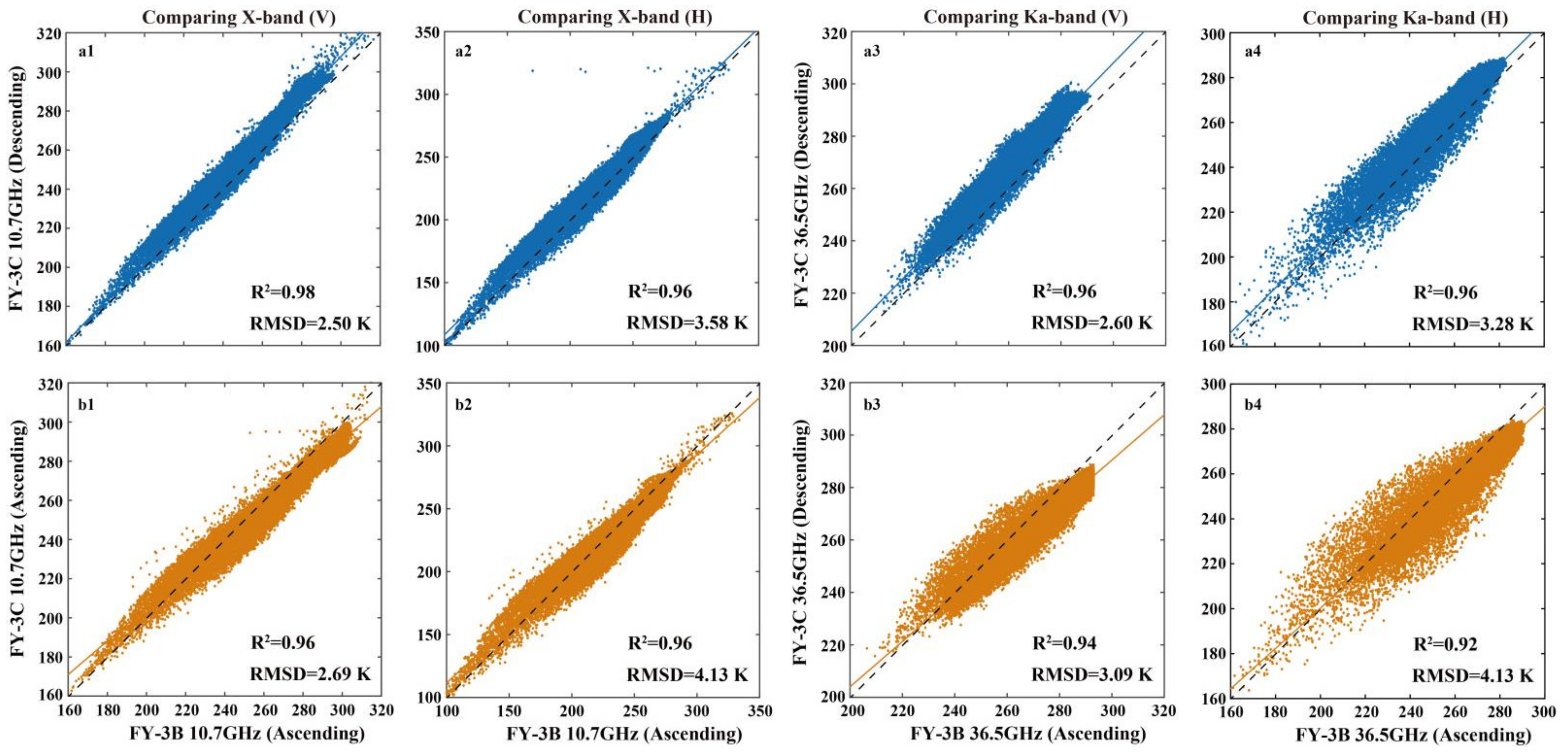
3.1. Comparison and Analysis of the FY-3B/3C Brightness Temperature

In order to develop continuous and consistent SM datasets from the FY-3B and FY-3C satellite observations, it is for their TB observations to be compared to determine whether a mutual calibration is needed. Parinussa et al. [85] showed the necessity of such mutual calibration, which has led to the consistency between SM retrieved from WindSat and AMSR-E. Here, the X-band data, mainly needed for SM retrieval, and Ka-band data, for LST retrieval, are selected and analyzed using the range of 60°S–60°N (Figure 2). Overall, there is a very good consistency between the two satellite observations. Nonetheless, it can be seen from the figure that the consistency of the descending TB data of the two sensors is slightly higher than that of the ascending data. For instance, in the case of Ka-band horizontal polarization, the coefficient of determination (R2) of TB descending path is 0.98, while the R2 of the ascending path is 0.96. Additionally, the R2 of X-band data is slightly higher than Ka-band data. Earlier studies have shown that the open water signals cause the scattered spread at the low ends of the Ka-band, with larger variation in observations close to midday, as shown by the FY3B ascending data in Figure 2 [10,86]. The RMSD calculation results (here, differences (RMSD) instead of errors (RMSE) are used because the comparison is just a relative difference between the two observations; RMSEs are used here in the case of TCA and comparisons with in situ, which are taken as ground truth) between the FY-3B and FY-3C TB data shown in Figure 2 show that the largest value (4.13 K) falls in the horizontal polarization of the X-band and Ka-band, demonstrating that the two satellites can be relied on for consistent long-term daily time series of SM and LST dynamics.

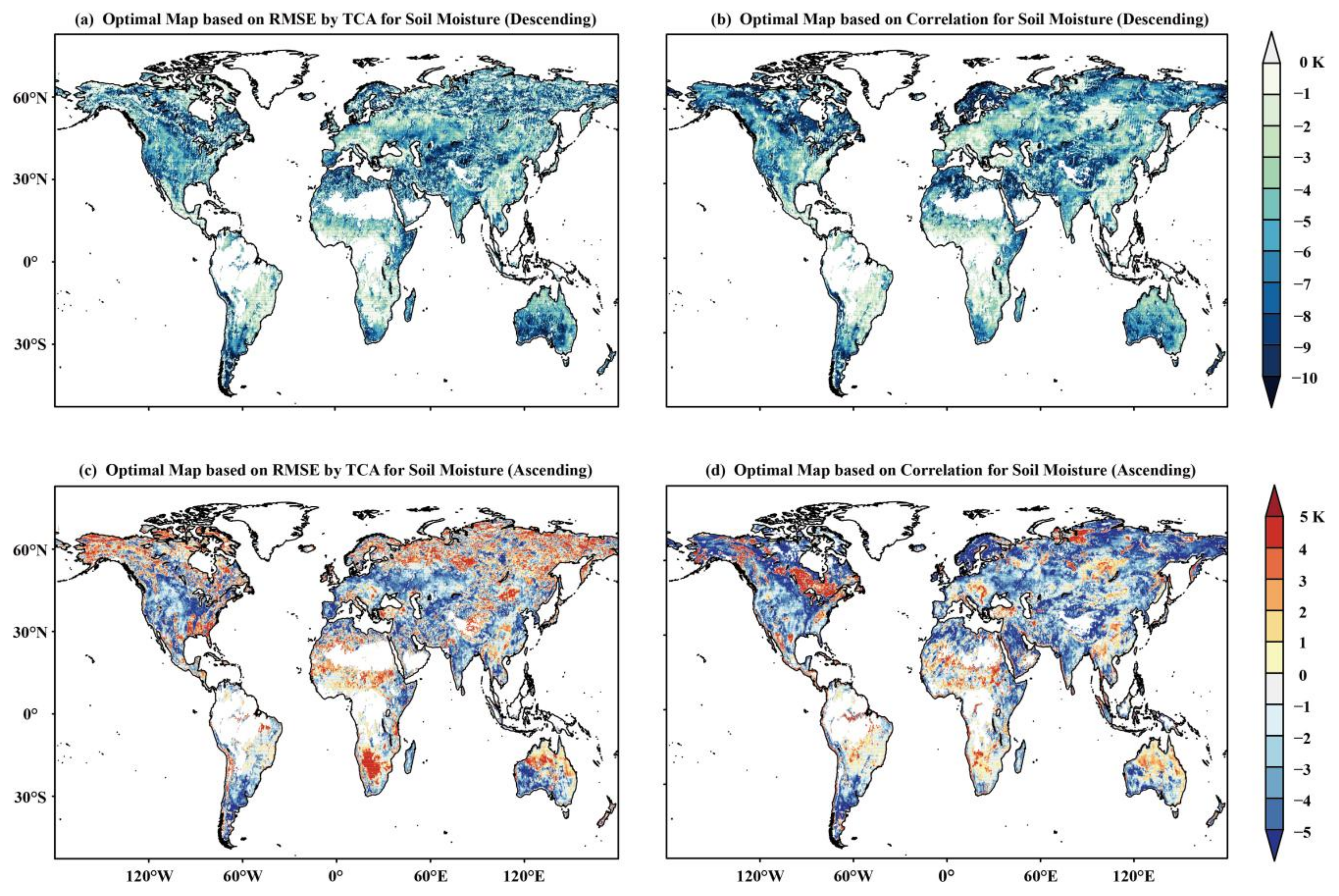
3.2. Global Optimization

Figure 3 presents the optimization for the LST bias scenario with the lowest SM bias. We applied TCA to all the SM scenarios to evaluate their relative qualities and obtain an optimal solution. A pixel-wise correlation analysis was also performed with each bias scenario and ERA5-Land SM as an added verification step. Figure 3a,c represent the lowest RMSE of SM based on different LST bias scenarios. Figure 3b,d represent the highest correlation of SM based on different LST bias scenarios. The bias scenarios of the descending LST are from −10 K (blue) to 0 K (gray), and the bias scenarios of the ascending LST are from −5 K (blue) to 5 K (red). Thus, the results in Figure 3 show which LST bias scenario per pixel produces the highest quality of soil moisture for the pixel. Our global optimization results show low-bias scenarios around the equator, whereas higher latitudes have higher-bias scenarios. Figure 3a shows the spatial distribution map of the bias scenario with the least TCA RMSE for SM in the FY-3C descending observations. The results show that the low-bias scenarios (low or high biases here refer to their absolute magnitudes) are generally found at locations at or near the equator. In contrast, high-bias scenarios are found near higher latitudes. These findings are consistent with the previous studies where SM retrievals from LPRM were found to have large biases in high latitude regions due to the region’s wet climate [87]. Hagan et al. [10] later capitalized on this to reduce LST biases by considering open water fraction in the grids. It is obvious from the results that no bias scenario presents an optimal solution for accurate SM estimates. The results also show that the LST scenario with the lowest bias does not necessarily produce the best quality of SM, which confirms the nonlinear relationship between SM and LST in the radiative transfer equation. Figure 3b shows the SM bias scenarios with the highest correlation coefficient with ERA5-Land SM. The results agree with the TCA RMSE in Figure 3a, which indicates that RMSE (TCA) is feasible as the basis for the optimization. A similar optimization routine was carried out with the ascending observations; however, optimal solutions were found within a bias scenario range from −5 K to 5 K. These significant differences between the bias ranges of the two acquisition times have been shown and elaborated by Lei et al. [88], who attributed the difference to how evapotranspiration is represented at the time of data acquisition. Figure 3c shows the optimal bias scenarios based on TCA, while Figure 3d shows the optimal solutions based on correlations with ERA5-Land. As noted with the descending results, the optimal solution does not lie with the 0 K scenarios or one particular scenario but within a spectrum of scenarios. Positive biases were found over the high latitudes and in the tropical regions. In contrast, the negative biases were found in the mid-latitudes, where the TCA and correlation-based optimal maps are not as high as the descending orbits results, suggesting that the accuracy for optimal solutions from descending orbits would be more significant than that from the ascending orbits.

3.3. Global Verification

As a final step, the LST of the optimal SM scenarios were used to obtain calibrated retrieval equations for both the ascending and descending TB of FY-3C by determining their optimal slope and offsets in the equations below. Equation (6) is the obtained calibrated LST retrieval equation for ascending TB, and Equation (7) is for the descending TB:

LST = 0.627 × Tb_asc (36.50 V) + 119.4 [K]

(6)

LST = 0.734 × Tb_desc (36.50 V) + 86.9 [K]

(7)

These equations are, thus, the proposed benchmark equations for retrieving LST from FY-3C. To quantify the improvements from this calibration process, TCA is applied to the SM retrievals from both the calibrated and un-calibrated (Figure 4a,b). Additionally, the correlation between the anomalies of the two SM retrievals and the ERA5-Land SM anomalies are also estimated (Figure 4c,d). Beyond these NDVI ranges, satellite SM loses skill and sensitivity to rainfall with a low signal-to-noise ratio in bone-dry regions. Figure 4 shows that more significant improvements are realized from the descending products than ascending products through the calibration process. The evolution of the TCA RMSE results is consistent with the skill of passive microwave-based SM retrievals reported in previous studies. The SM observations lose skill with increasing vegetation density, as seen in the descending (Figure 4a) and ascending data (Figure 4b). This difference in the quality of the SM retrieval after calibration could be attributed to an assumption in LPRM, where the vegetation temperature is considered equivalent to the bare LST [45,88]. Here, the assumption works best when there is increased thermal equilibrium such that the temperature at the top of the canopy is equivalent to the temperature at the surface of the land. In the daytime, the transpiration process affects the canopy temperature, leading to the cooling of the canopy. However, the LST generally warms up [89]. Therefore, different LST inputs of different observation times will affect the retrieval quality. Further improvement of daytime observations will lead to significant progress, while nighttime observation quality may not be obvious. As a result, optimizing the un-calibrated retrieval realizes more obvious improvements in the descending observations (taken at 10:00) than ascending observations (taken at 22:00). The correlation analysis results for descending (Figure 4c) and ascending data (Figure 4d) also demonstrate that the calibrated improvement is more significant in the descending observations. The lower correlations in NDVI < 0.4 regions result from the reduced sensitivities in the satellite observations due to insufficient precipitation in the regions [28,47]. Nonetheless, higher correlations are found over regions of low vegetation densities in the ascending product and reduced skill with increasing vegetation density (NDVI > 0.4) for both products, thus validating the assumption’s impact, as discussed above.

Next, an independent evaluation of the calibrated datasets with the ISMN in situ SM observations is also carried out. Here, the skills of the calibrated ascending and descending FY-3C SM retrievals are assessed to understand their strengths and weaknesses. The relevant information of the selected SM networks is described in detail in Table 1. Figure 5 shows the RMSE and correlation analysis of the two satellite products with the in situ datasets at their corresponding times. The results are presented for each network, which comprises multiple stations. The RMSE values are mostly concentrated between 0.05–0.15 m³ m⁻³, and the correlation coefficient values are mostly within 0.4–0.7. Generally, the ascending mean errors (ranging between 0.03–0.05 m³ m⁻³) are lower than the descending mean errors (ranging between 0.04–0.05 m³ m⁻³) for all the networks except SMOSMANIA. Additionally, the mean correlations are also higher for the ascending than the descending datasets. As mentioned above, this may be because ascending observations (nighttime) are less affected by vegetation transpiration than descending orbital observations (daytime); therefore, the data from ascending observations (nighttime) are more accurate. Figure 5 shows that the AMMA-CATCH SM in Africa shows the lowest errors with high correlations for both the ascending and descending data. Because this SM network is in the arid region with a low vegetation coverage, it has less influence on the SM retrieval. Given that this region is significantly challenged by lack of observation data; it behooves both scientific research and application of these datasets to have such good qualities. On the other hand, the lowest performance of the datasets is found with the SMOSMANIA network located in the south of France, which has the highest errors and lowest correlations. This SM network is located near open water, affecting the retrieval quality. Additionally, high vegetation coverage in the region also contributes to the reduced qualities observed. Nonetheless, the results show that the calibrated FY-3C SM datasets are reliable on the whole, having relatively low errors (Figure 5a) and good temporal correlations (Figure 5b). Furthermore, the highly varying qualities between the networks also demonstrate a spatial dependency. This is explored in detail in the next section.

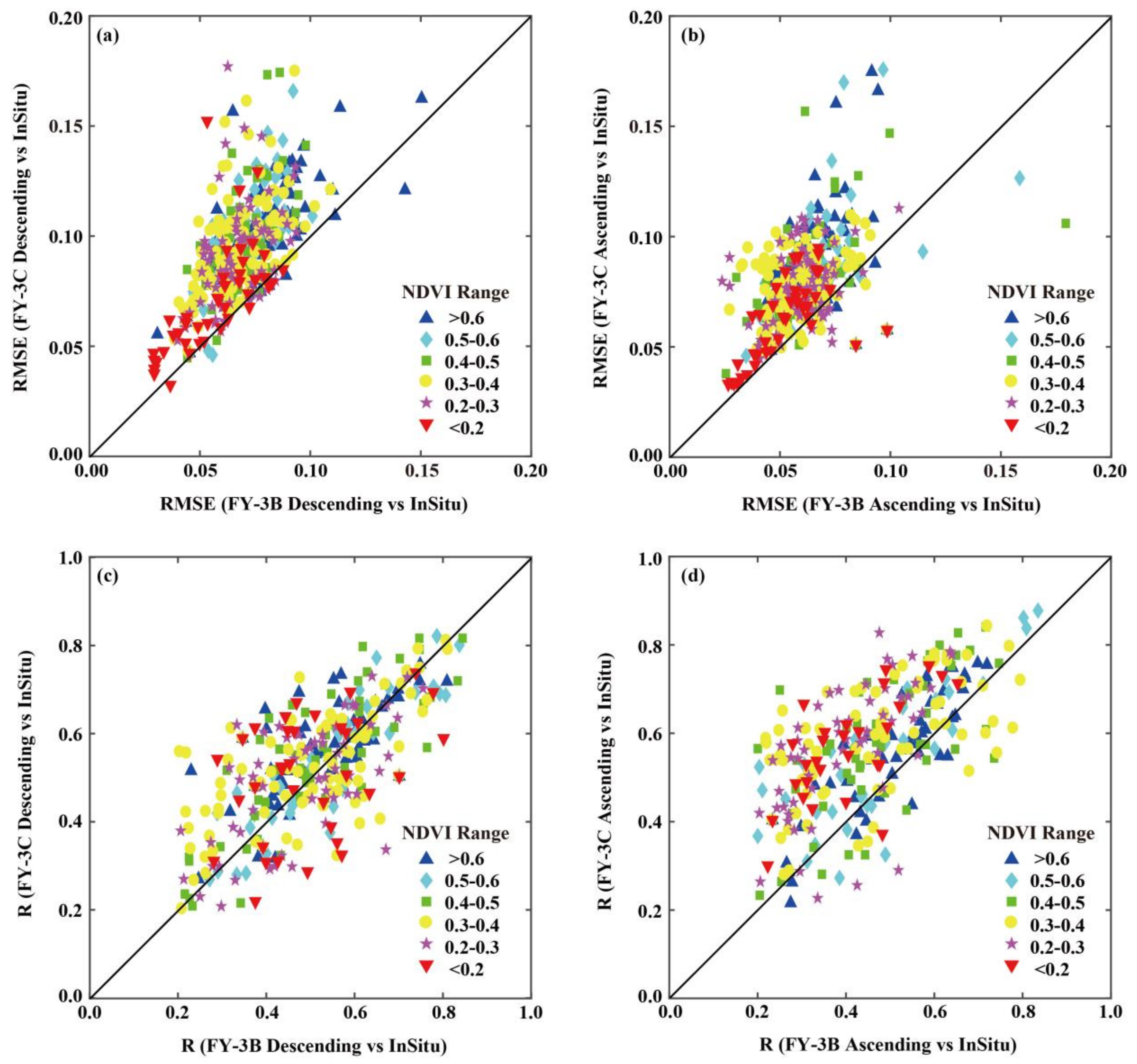
3.4. Inter-Comparison of FY-3B and FY-3C Products

As mentioned above, the accuracy of SM retrievals has been found to vary as a function of vegetation distribution. Here, the SM anomalies of FY-3C are inter-compared with that of FY-3B to understand their consistency over different NDVI distributions based on the in situ observations, as shown in Figure 6. The results show that vegetation density impacts the errors of the ascending and descending SM estimates of both datasets. Figure 4a,b and Figure 6a,b also show that low vegetation areas have the lowest errors, while dense vegetation areas have the largest errors. Furthermore, most errors are found above the 1:1 line, indicating slightly larger in FY-3C than in FY-3B. In Figure 6c,d, on the other hand, the correlations are almost evenly generally scattered around the 1:1 line, showing that their temporal consistencies are very similar. In addition, higher correlations are found in the ascending datasets of FY-3C, since a higher density of the results are found above the 1:1 line in Figure 6d. Higher correlations are found in the dense vegetation areas within the descending FY-3C datasets, and higher correlations are also found in the low vegetation areas within the ascending FY-3C datasets. Generally, we expect that because of the observation time of FY-3C, we would find lower qualities in the dense vegetation areas than FY-3B due to higher thermal equilibrium in FY-3B at night. However, FY-3C appears to have higher correlations (Figure 6c), although larger RMSEs are also found there (Figure 6a). As noted in the optimal maps from Figure 3a,b, the optimization would also improve the correlations of FY-3C, especially in the dense vegetation regions where thermal equilibrium is generally reduced due to transpiration. Higher correlations in the low vegetation areas of the ascending observations of FY-3C in Figure 6d are consistent with previous studies that also found higher correlations in nighttime observations [47]. Overall, Figure 6 distinctly demonstrates a very high consistency between the two satellite retrievals for both orbits, which is essential for developing long-term records from both observations.

In aiming towards including the SM retrievals from FY-3B and FY-3C in long-term records, it is important to investigate how their strengths can be leveraged to describe daily SM dynamics. Additionally, it is helpful to identify regions where either retrieval can be relied on more to explain daily soil moisture variability. To do this, TCA is applied to the SM anomalies from both satellites observations and the regional differences are shown globally for both the ascending and descending products (Figure 7a,b). Here, red-colored regions imply lower errors in FY-3B, and blue-colored regions imply lower errors in FY-3C. As a routine in LPRM, very dense vegetation regions are masked out. Overall, the results show that the skill of FY-3B in capturing daily SM dynamics is better in descending products, while FY-3C is better in the ascending product. A strong contrast can be seen from Figure 7a,b, especially from the mid-latitudes in the northern hemisphere (NH) to the southern hemisphere (SH) that in regions where FY-3B has higher accuracies in descending products, the FY-3C picks that up in the ascending products. It is worth noting that the FY-3B is shown to dominate the high latitudes, eastern North America, and Australia in both the ascending and descending products from the TCA results. A similar accuracy assessment is done based on correlation analysis, as shown in Figure 7c,d. The results show a strong agreement with the TCA results. Higher accuracies are reported in FY-3C over high latitudes over the NH in the descending products, with higher accuracies realized in NH mid-latitudes all through the SH (Figure 7c). The opposite distribution of the accuracies between the two satellite observations is seen in the ascending products (Figure 7c). These results highlight how the two observation sources complement each other in capturing daily SM dynamics.

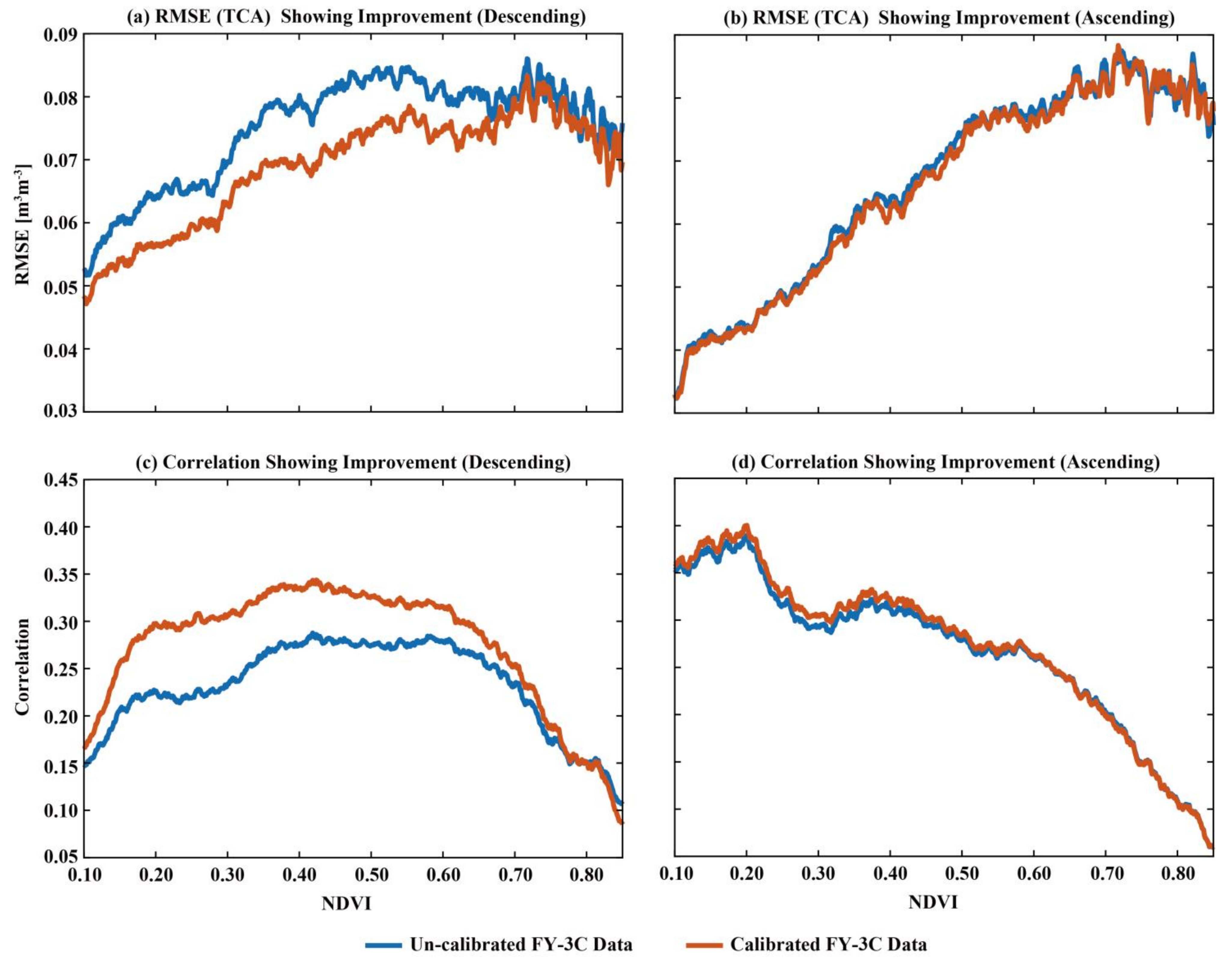
3.5. Evaluation of Combination Results

To demonstrate the added value of the combined product of merging the FY-3B and FY-3C ascending/descending observations, it is evaluated with in situ SM and compared with the parent products (FY-3B and FY-3C). In this study, the in situ data from 2014 to 2015 are selected for verification. The latitude and longitude positions of the chosen grid in the Figure 8 are 118°W, 42°N, and the corresponding SM site name is SNOTEL_DISATERPEAK. This site is located in the Midwest region of the United States. The timeseries of this site is more complete, which is easy to compare with the retrieval and combined data. Figure 8a,b shows the time series of a chosen pixel for both the descending and ascending products, respectively. The results demonstrate that the merged product has accurately captured the variability of in situ soil moisture. A clear increased performance is seen in the combined product compared to the parent products. Apart from capturing the seasonal variability, significant precipitation events seen in the in situ data are also well captured in the combined product, which verifies the validity of the parent products as well.

As a final verification step, all matching pixels in the three products: two parents and the combined, to the in situ observations, are compared based as a function of vegetation based on NDVI. This final evaluation aims to understand the relative strengths of the parent products that are leveraged in the combined product. As was done in the above analysis, NDVI > 0.1 to NDVI < 0.75 are used, since satellite SM loses skill beyond these boundaries [47]. In Figure 9, the blue and red lines represent the FY-3B and FY-3C SM products, respectively, while the black line presents the combined product. As was reported by Hagan et al. [40], improvements in the mean differences, here quantified with RMSEs with the in situ observations, are attributed to the normalization step. Figure 9a,b both show that the RMSEs are reduced in the combined products over all vegetation density scenarios. This partly shows the biases within the parent products attributed to a limitation of LPRM. Future studies could incorporate improvement schemes, such as improving the LST inputs as proposed by Hagan et al. [10] or applying a dynamic vegetation correction as suggested by Parinussa et al. [34], to reduce biases and errors within the retrievals from LPRM. Figure 9c,d show the added value of the merging process to maximize the correlations in the combined product. Significant improvements are realized in the combined product over most vegetation density scenarios, especially between NDVI > 0.2 and NDVI < 0.7. This attests to the importance of a co-usage of these products for both scientific research and applications. Both FY-3B and FY-3C clearly have individual merits that, when combined, have very promising uses. More importantly, the combined usage is essential to developing long-term soil moisture records. The results in Figure 9 also show that while FY-3B tends to have lower RMSE, FY-3C tends to have higher correlations in both the ascending and descending products. This is very important to note, especially when it comes to studying physical processes within the climate. Some processes would benefit from accurate means, and others would benefit from accurate temporal variability. Furthermore, this sheds some light on a possible benefit of SM observations at these overpass times of the two satellite observations.

4. Conclusions

SM can regulate the exchange of water vapor and energy between the land and the atmosphere by changing surface fluxes. Therefore, SM data can help predict extreme events, such as droughts, floods, and heatwaves [3,13]. Microwave remote sensing technology is one of the most effective ways to monitor SM dynamics on a regional and global scale [90]. In this paper, we used China Meteorological Administration’s FY-3C TB to solve for an optimal solution of SM by retrieving the LST input used in LPRM. The obtained soil moisture product was routinely evaluated using both global in situ and high-quality reanalysis SM products to understand its relative qualities. We also examined the complementarity of FY-3C and FY-3B satellite SM observations for obtaining consistent long-term SM records. Our conclusions are as follows.

The evaluation of the TB from the MWRI onboard FY-3B and FY-3C under the different polarization modes of X- and Ka-band suggests that the TB values of the two satellite platforms are consistent with correlation coefficients above 0.95. The consistency of TB data in the descending orbits is slightly higher than that in the ascending orbit. The X-band data showed a higher consistency than the Ka-band data in our comparison. Our overall results demonstrate the potential usefulness of the combined applications of FY-3B and FY-3C satellite observations.

Unlike FY-3B, FY-3C comes at a different observation time of the day, implying the need to tune the SM retrieval algorithm, the LPRM, to fit the observation time of FY-3C. We adopted the LST retrieval approach proposed by Holmes et al. [45] to obtain the un-calibrated LST retrieval equations. However, because of the nonlinear linkage between LST and SM, optimizing the LST inputs was essential to obtain an optimal solution for SM. Following Parinussa et al. [47], the algorithm was optimized using the TCA method for both ascending and descending datasets of FY-3C. Comparison of the correlation coefficients and the RMSE (TCA) of un-calibrated and calibrated results showed obvious improvements in the descending (daytime) data, and a slight improvement in the ascending (nighttime) data, possibly due to increased thermal equilibrium of the nighttime SM and canopy temperature. Further evaluations of the improved FY-3C SM anomalies using the ISMN in situ data, we found the RMSE values were concentrated between 0.05–0.15 m³ m⁻³ and the correlation coefficient between 0.4–0.7, although better skill was found in the ascending SM product. Additionally, the evaluations also showed that, similar to the FY-3B, the FY-3C SM improves skill with decreasing vegetation density.

In a final step, we aimed to unravel the complementarity of FY-3B and FY-3C SM by comparing their individual and combined potentials [84] relative to in situ observations. When we combined the daytime and nighttime SM products separately, the results showed superior skill to capture SM dynamics than the individual products, since they leveraged the best of each product. Each product had its unique advantage over space-time and time, demonstrating the FY-3C series can add value to existing SM records similar to the CCI.

This study has found that the FY-3C is useful in filling gaps in the global observational records of SM, LST, and VOD, for which there are little to no observations available. Furthermore, the FY-3C provides observations at a unique time that was initially unavailable, which makes it useful to understand land surface processes. Future studies are needed to extend this framework to the recently launched FY-3D satellite for global soil moisture observation to serve as a successor of the FY-3B and FY-3C satellites.

References

1. Dobriyal, P.; Qureshi, A.; Badola, R.; Hussain, S.A. A review of the methods available for estimating soil moisture and its implications for water resource management. J. Hydrol. 2012, 458–459, 110–117. [Google Scholar] [CrossRef]
2. Petropoulos, G.P.; Ireland, G.; Barrett, B. Surface soil moisture retrievals from remote sensing: Current status, products & future trends. Phys. Chem. Earth 2015, 83–84, 36–56. [Google Scholar]
3. Seneviratne, S.I.; Corti, T.; Davin, E.L.; Hirschi, M.; Jaeger, E.B.; Lehner, I.; Orlowsky, B.; Teuling, A.J. Investigating soil moisture–climate interactions in a changing climate: A review. Earth-Sci. Rev. 2010, 99, 125–161. [Google Scholar] [CrossRef]
4. Entekhabi, D.; Njoku, E.G.; O’Neill, P.E.; Kellogg, K.H.; Crow, W.T.; Edelstein, W.N.; Entin, J.K.; Goodman, S.D.; Jackson, T.J.; Johnson, J.; et al. The Soil Moisture Active and Passive (SMAP) mission. Proc. IEEE 2010, 98, 704–716. [Google Scholar] [CrossRef]
5. Zheng, X.M.; Bai, Y.; Jiang, T.; Zhao, X.; Zhao, K. Evaluation of SMAP Passive Soil Moisture Products Using In-Situ Data from a Dense Observation Network. In Proceedings of the IGARSS 2019-2019 IEEE International Geoscience and Remote Sensing Symposium, Yokohama, Japan, 28 July–2 August 2019. [Google Scholar]
6. Shi, J.C.; Du, Y.; Du, J.Y.; Jiang, L.M.; Chai, L.N.; Mao, K.B.; Xu, P.; Ni, W.J.; Xiong, C.; Liu, Q.; et al. Progresses on microwave remote sensing of land surface parameters. Sci. China Earth Sci. 2012, 55, 1052–1078. [Google Scholar] [CrossRef]
7. Magagi, R.; Berg, A.A.; Goïta, K.; Bélair, S.; Jackson, T.J.; Toth, B.; Walker, A.; McNairn, H.; O’Neill, P.E.; Moghaddam, M.; et al. Experiment for Soil Moisture in 2010 (CanEx-SM10): Overview and Preliminary Results. IEEE Trans. Geosci. Remote Sens. 2013, 51, 347–363. [Google Scholar] [CrossRef] [Green Version]
8. Draper, C.; Reichle, R.H. Assimilation of Satellite Soil Moisture for Improved Atmospheric Reanalyses. Mon. Wea. Rev. 2019, 147, 2163–2188. [Google Scholar] [CrossRef]
9. Song, P.L.; Huang, J.F.; Mansaray, L.R.; Wen, H.Y.; Wu, H.Y.; Liu, Z.X.; Wang, X.Z. An Improved Soil Moisture Retrieval Algorithm Based on the Land Parameter Retrieval Model for Water–Land Mixed Pixels Using AMSR-E Data. IEEE Trans. Geosci. Remote Sens. 2019, 57, 7643–7657. [Google Scholar] [CrossRef]
10. Hagan, D.F.T.; Wang, G.J.; Parinussa, R.M.; Shi, X. Inter-comparing and improving land surface temperature estimates from passive microwaves over the Jiangsu province of the People’s Republic of China. Int. J. Remote Sens. 2019, 40, 5563–5584. [Google Scholar] [CrossRef]
11. Bolten, J.D.; Crow, W.T. Improved prediction of quasi-global vegetation conditions using remotely-sensed surface soil moisture. Geophys. Res. Lett. 2012, 39, L19406. [Google Scholar] [CrossRef] [Green Version]
12. Holzman, M.E.; Rivasa, R.; Piccolo, M.C. Estimating soil moisture and the relationship with crop yield using surface temperature and vegetation index. Int. J. Appl. Earth Obs. 2014, 28, 181–192. [Google Scholar] [CrossRef]
13. McColl, K.A.; Alemohammad, S.H.; Akbar, R.; Konings, A.G.; Yueh, S.; Entekhabi, D. The global distribution and dynamics of surface soil moisture. Nat. Geosci. 2017, 10, 100–104. [Google Scholar] [CrossRef]
14. Yang, G.; Guo, P.; Li, X.C.; Wan, H.; Meng, C.H.; Wang, B. Assessment with remotely sensed soil moisture products and ground-based observations over three dense networks. Earth Sci. Inform. 2020, 13, 663–679. [Google Scholar] [CrossRef]
15. Pablos, M.; Martínez-Fernández, J.; Piles, M.; Sánchez, N.; Vall-llossera, M.; Camps, A. Multi-T emporal Evaluation of Soil Moisture and Land Surface T emperature Dynamics Using in Situ and Satellite Observations. Remote Sens. 2016, 8, 587. [Google Scholar] [CrossRef] [Green Version]
16. Njoku, E.G.; Jackson, T.J.; Lakshmi, V.; Chan, T.K.; Nghiem, S.V. Soil moisture retrieval from AMSR-E. IEEE Trans. Geosci. Remote Sens. 2003, 41, 215–229. [Google Scholar] [CrossRef]
17. Wigneron, J.P.; Kerr, Y.; Waldteufel, P.; Saleh, K.; Escorihuela, M.J.; Richaume, P.; Ferrazzoli, P.; de Rosnay, P.; Gurney, R.; Calvet, J.C.; et al. L-band Microwave Emission of the Biosphere (L-MEB) Model: Description and calibration against experimental data sets over crop fields. Remote Sens. Environ. 2007, 107, 639–655. [Google Scholar] [CrossRef]
18. Owe, M.; de Jeu, R.; Holmes, T. Multisensor historical climatology of satellite-derived global land surface moisture. J. Geophys. Res. 2008, 113, F01002. [Google Scholar] [CrossRef]
19. Kerr, Y.H.; Waldteufel, P.; Wigneron, J.P.; Delwart, S.; Cabot, F.; Boutin, J.; Escorihuela, M.; Font, J.; Reul, N.; Gruhier, C.; et al. The SMOS Mission: New Tool for Monitoring Key Elements of the Global Water Cycle. Proc. IEEE 2010, 98, 666–687. [Google Scholar] [CrossRef] [Green Version]
20. Kim, S.; Zhang, R.Z.; Pham, H.; Sharma, A. A Review of Satellite-Derived Soil Moisture and Its Usage for Flood Estimation. Remote Sens. Earth Syst. Sci. 2019, 2, 225–246. [Google Scholar] [CrossRef]
21. Karthikeyan, L.; Pan, M.; Wanders, N.; Kumar, D.N.; Wood, E.F. Four decades of microwave satellite soil moisture observations: Part 1. A review of retrieval algorithms. Adv. Water Resour. 2017, 109, 106–120. [Google Scholar] [CrossRef]
22. Karthikeyan, L.; Pan, M.; Wanders, N.; Kumar, D.N.; Wood, E.F. Four decades of microwave satellite soil moisture observations: Part 2. Product validation and inter-satellite comparisons. Adv. Water Resour. 2017, 109, 236–252. [Google Scholar] [CrossRef]
23. Chang, A.T.C.; Atwater, S.G.; Salomonson, V.V.; Estes, J.E.; Simonett, D.S.; Bryan, M.L. L-Band Radar Sensing of Soil Moisture. IEEE Trans. Geosci. Remote Sens. 1980, 4, 303–310. [Google Scholar] [CrossRef] [Green Version]
24. Shi, J.; Jiang, L.; Zhang, L.; Chen, K.S.; Wigneron, J.P.; Chanzy, A. A parameterized multifrequency-polarization surface emission model. IEEE Trans. Geosci. Remote Sens. 2005, 43, 2831–2841. [Google Scholar]
25. Shi, J.; Jiang, L.; Zhang, L.; Chen, K.S.; Wigneron, J.P.; Chanzy, A.; Jackson, T.J. Physically Based Estimation of Bare-Surface Soil Moisture With the Passive Radiometers. IEEE Trans. Geosci. Remote Sens. 2006, 44, 3145–3153. [Google Scholar] [CrossRef]
26. Wigneron, J.P.; Chanzy, A.; Kerr, Y.H.; Lawrence, H.; Shi, J.; Escorihuela, M.J.; Mironov, V.; Mialon, A.; Demontoux, F.; Rosnay, P.; et al. Evaluating an Improved Parameterization of the Soil Emission in L-MEB. IEEE Trans. Geosci. Remote Sens. 2011, 49, 1177–1189. [Google Scholar] [CrossRef]
27. Fujii, H.; Koike, T.; Imaoka, K. Improvement of the AMSR-E Algorithm for Soil Moisture Estimationby Introducing a Fractional Vegetation Coverage DatasetDerived from MODIS Data. J. Remote Sens. Soc. Jpn. 2009, 29, 282–292. [Google Scholar]
28. van der Schalie, R.; de Jeu, R.A.M.; Kerr, Y.H.; Wigneron, J.P.; Rodríguez-Fernández, N.J.; Al-Yaari, A.; Parinussa, R.M.; Mecklenburg, S.; Drusch, M. The merging of radiative transfer based surface soil moisture data from SMOS and AMSR-E. Remote Sens. Environ. 2017, 189–193. [Google Scholar] [CrossRef]
29. Jing, W.L.; Song, J.; Zhao, X.D. A Comparison of ECV and SMOS Soil Moisture Products Based on OzNet Monitoring Network. Remote Sens. 2018, 10, 703. [Google Scholar] [CrossRef] [Green Version]
30. Owe, M.; de Jeu, R.; Walker, J. A Methodology for Surface Soil Moisture and Vegetation Optical Depth Retrieval Using the Microwave Polarization Difference Index. IEEE Trans. Geosci. Remote Sens. 2001, 39, 1643–1654. [Google Scholar] [CrossRef] [Green Version]
31. De Jeu, R.; Holmes, T.; Parinussa, R.; Owe, M. A spatially coherent global soil moisture product with improved temporal resolution. J. Hydrol. 2014, 516, 284–296. [Google Scholar] [CrossRef]
32. Van der Schalie, R.; Parinussa, R.M.; Renzullo, L.J.; van Dijk, A.I.J.M.; Su, C.H.; De Jeu, R.A.M. SMOS soil moisture retrievals using the land parameter retrieval model: Evaluation over the Murrumbidgee Catchment, southeast Australia. Remote Sens. Environ. 2015, 163, 70–79. [Google Scholar] [CrossRef]
33. Van der Schalie, R.; Kerr, Y.H.; Wigneron, J.P.; Rodríguez-Fernández, N.J.; Al-Yaari, A.; De Jeu, R.A.M. Global SMOS Soil Moisture Retrievals from The Land Parameter Retrieval Model. Int. J. Appl. Earth Obs. Geoinf. 2016, 45, 125–134. [Google Scholar] [CrossRef]
34. Parinussa, R.M.; Wang, G.J.; Liu, Y.; Lou, D.; Hagan, D.F.T.; Zhan, M.J.; Su, B.D.; Jiang, T. Improved surface soil moisture anomalies from Fengyun-3B over the Jiangxi province of the People’s Republic of China. Int. J. Remote Sens. 2018, 39, 8950–8962. [Google Scholar] [CrossRef]
35. Paloscia, S.; Macelloni, G.; Santi, E.; Koike, T. A multifrequency algorithm for the retrieval of soil moisture on a largescale using microwave data from SMMR and SSM/I satellites. IEEE Trans. Geosci. Remote Sens. 2001, 39, 1655–1661. [Google Scholar] [CrossRef]
36. Li, L.; Gaiser, P.W.; Gao, B.C.; Bevilacqua, R.M.; Jackson, T.J.; Njoku, E.G.; Rudiger, C.; Calvet, J.C.; Bindlish, R. WindSat Global Soil Moisture Retrieval and Validation. IEEE Trans. Geosci. Remote Sens. 2010, 48, 2224–2241. [Google Scholar] [CrossRef]
37. Du, J.Y.; Kimball, J.S.; Shi, J.C.; Jones, L.A.; Wu, S.L.; Sun, R.J.; Yang, H. Inter-Calibration of Satellite Passive Microwave Land Observations from AMSR-E and AMSR2 Using Overlapping FY3B-MWRI Sensor Measurements. Remote Sens. 2014, 6, 8594–8616. [Google Scholar] [CrossRef] [Green Version]
38. Parinussa, R.M.; Wang, G.J.; Liu, Y.Y.; Hagan, D.F.T.; Lin, F.F.; van der Schalie, R.; De Jeu, R.A.M. The Evaluation of Single-Sensor Surface Soil Moisture Anomalies over the Mainland of the People’s Republic of China. Remote Sens. 2017, 9, 149. [Google Scholar] [CrossRef] [Green Version]
39. Kerr, Y.H.; Al-Yaari, A.; Rodriguez-Fernandez, N.; Parrens, M.; Molero, B.; Leroux, D.; Bircher, S.; Mahmoodi, A.; Mialon, A.; Richaume, P.; et al. Overview of SMOS performance in terms of global soil moisture monitoring after six years in operation. Remote Sens. Environ. 2016, 180, 40–63. [Google Scholar] [CrossRef]
40. Hagan, D.F.T.; Liu, Y.; Ullah, W.; Wang, G.J.; Kim, S.; Parinussa, R.M.; Bhatti, A.S.; Ma, X.W.; Jiang, T.; Su, B.D. Maximizing Temporal Correlations in Long-Term Global Satellite Soil Moisture Data-Merging. Remote Sens. 2020, 12, 2164. [Google Scholar] [CrossRef]
41. Yang, H.; Shi, J. On the Estimation of Land Surface Parameters by Using FY-3 Microwave Radiometer Imager. Remote Sens. Technol. Appl. 2005, 1, 194–200. [Google Scholar]
42. Bao, Y.S.; Mao, F.; Min, J.Z. Retrieval of bare soil moisture from FY-3B/MWRI data. Remote Sens. Land Resour. 2014, 26, 131–137. [Google Scholar]
43. Hagan, D.F.T.; Parinussa, R.M.; Wang, G.J.; Draper, C.S. An Evaluation of Soil Moisture Anomalies from Global Model-Based Datasets over the People’s Republic of China. Water 2020, 12, 117. [Google Scholar] [CrossRef] [Green Version]
44. Scanlon, T.; Dorigo, W.; Preimesberger, W.; van der Schalie, R.; Hirschi, M.; van der Vliet, M.; Moesinger, L.; Rodriguez-Fernandez, N.; Pasik, A.; Kidd, R.; et al. ESA CCI and C3S Soil Moisture Products: Generation and Quality Assurance, EGU General Assembly. In Proceedings of the ESA CCI Soil Moisture, Vienna, Austria, 4–13 April 2018. EGU21-9796. [Google Scholar]
45. Holmes, T.R.H.; De Jeu, R.; Owe, M.; Dolman, A.J. Land surface temperature from Ka band (37 GHz) passive microwave observations. J. Geophys. Res. 2009, 114, D04113. [Google Scholar] [CrossRef] [Green Version]
46. Holmes, T.R.H.; Crow, W.T.; Tugrul Yilmaz, M.; Jackson, T.J.; Basara, J.B. Enhancing model-based land surface temperature estimates using multiplatform microwave observations. J. Geophys. Res. Atmos. 2013, 118, 577–591. [Google Scholar] [CrossRef]
47. Parinussa, R.M.; De Jeu, R.A.M.; van der Schalie, R.; Crow, W.T.; Lei, F.N.; Holmes, T.R.H. A Quasi-Global Approach to Improve Day-Time Satellite Surface Soil Moisture Anomalies through the Land Surface Temperature Input. Climate 2016, 4, 50. [Google Scholar] [CrossRef] [Green Version]
48. Mladenova, I.E.; Jackson, T.J.; Njoku, E.; Bindlish, R.; Chan, S.; Cosh, M.H.; Holmes, T.R.H.; de Jeu, R.A.M.; Jones, L.; Kimball, J.; et al. Remote monitoring of soil moisture using passive microwave-based techniques-Theoretical basis and overview of selected algorithms for AMSR-E. Remote Sens. Environ. 2014, 144, 197–213. [Google Scholar] [CrossRef]
49. Kang, C.S.; Zhao, T.J.; Shi, J.C.; Cosh, M.H.; Chen, Y.Y.; Starks, P.J.; Holifield, C.C.; Wu, S.L.; Sun, R.J.; Zheng, J.Y. Global Soil Moisture Retrievals from the Chinese FY-3D Microwave Radiation Imager. IEEE Trans. Geosci. Remote Sens. 2020, 99, 1–15. [Google Scholar] [CrossRef]
50. Wang, L.; Fang, S.B.; Pei, Z.F.; Zhu, Y.C.; Khoi, D.N.; Han, W. Using FengYun-3C VSM Data and Multivariate Models to Estimate Land Surface Soil Moisture. Remote Sens. 2020, 12, 1038. [Google Scholar] [CrossRef] [Green Version]
51. Parinussa, R.M.; Wang, G.; Holmes, T.R.H.; Liu, Y.Y.; Dolman, A.J.; de Jeu, R.A.M.; Jiang, T.; Zhang, P.; Shi, J. Global surface soil moisture from the Microwave Radiation Imager onboard the Fengyun-3B satellite. Int. J. Remote Sens. 2014, 35, 7007–7029. [Google Scholar] [CrossRef]
52. Zhu, Y.C.; Li, X.; Pearson, S.; Wu, D.L.; Sun, R.J.; Johnson, S.; Wheeler, J.; Fang, S.B. Evaluation of Fengyun-3C Soil Moisture Products Using In-Situ Data from the Chinese Automatic Soil Moisture Observation Stations: A Case Study in Henan Province, China. Water 2019, 11, 248. [Google Scholar] [CrossRef] [Green Version]
53. Dee, D.P.; Uppala, S.M.; Simmons, A.J.; Berrisford, P.; Poli, P.; Kobayashi, S.; Andrae, U.; Balmaseda, M.A.; Balsamo, G.; Bauer, P.; et al. The ERA-Interim reanalysis: Configuration and performance of the data assimilation system. Q. J. R. Meteorol. Soc. 2011, 137, 553–597. [Google Scholar] [CrossRef]
54. Albergel, C.; Dutra, E.; Munier, S.; Calvet, J.; Munoz-Sabater, J.; De Rosnay, P.; Balsamo, G. ERA-5 and ERA-Interim driven ISBA land surface model simulations: Which one performs better? Hydrol. Earth Syst. Sci. 2018, 22, 3515–3532. [Google Scholar] [CrossRef] [Green Version]
55. Olauson, J. ERA5: The new champion of wind power modelling? Renew. Energy 2018, 126, 322–331. [Google Scholar] [CrossRef] [Green Version]
56. Johannsen, F.; Ermida, S.; Martins, J.P.A.; Trigo, I.F.; Nogueira, M.; Dutra, E. Cold Bias of ERA5 Summertime Daily Maximum Land Surface Temperature over Iberian Peninsula. Remote Sens. 2019, 11, 2570. [Google Scholar] [CrossRef] [Green Version]
57. Hersbach, H.; Bell, B.; Berrisford, P.; Hirahara, S.; Horányi, A.; Muñoz-Sabater, J.; Nicolas, J.; Peubey, C.; Radu, R.; Schepers, D.; et al. The ERA5 Global Reanalysis. Q. J. R. Meteor. Soc. 2020, 14, 1999–2046. [Google Scholar] [CrossRef]
58. Wu, Z.Y.; Feng, H.H.; He, H.; Zhou, J.H.; Zhang, Y.L. Evaluation of Soil Moisture Climatology and Anomaly Components Derived From ERA5-Land and GLDAS-2.1 in China. Water Resour. Manag. 2021, 35, 629–643. [Google Scholar] [CrossRef]
59. Liu, Y.W.; Liu, Y.B.; Wang, W. Inter-comparison of satellite-retrieved and Global Land Data Assimilation System-simulated soil moisture datasets for global drought analysis. Remote Sens. Environ. 2019, 220, 1–18. [Google Scholar] [CrossRef]
60. Dorigo, W.A.; Xaver, A.; Vreugdenhil, M.; Gruber, A.; Hegyiová, A.; Sanchis-Dufau, A.D.; Zamojski, D.; Cordes, C.; Wagner, W.; Drusch, M. Global Automated Quality Control of In Situ Soil Moisture Data from the International Soil Moisture Network. Vadose Zone Hydrol. 2013, 12, 1–21. [Google Scholar] [CrossRef]
61. Dorigo, W.; Wagner, W.; Albergel, C.; Albrecht, F.; Balsamo, G.; Brocca, L.; Chung, D.; Ertl, M.; Forkel, M.; Gruber, A.; et al. ESA CCI Soil Moisture for improved Earth system understanding: State-of-the art and future directions. Remote Sens. Environ. 2017, 203, 185–215. [Google Scholar] [CrossRef]
62. Kim, H.; Parinussa, R.; Konings, A.G.; Wagner, W.; Cosh, M.H.; Lakshmi, V.; Zohaib, M.; Choi, M. Global-scale assessment and combination of SMAP with ASCAT (active) and AMSR2 (passive) soil moisture products. Remote Sens. Environ. 2018, 204, 260–275. [Google Scholar] [CrossRef]
63. Dorigo, W.; Himmelbauer, I.; Aberer, D.; Schremmer, L.; Petrakovic, I.; Zappa, L.; Preimesberger, W.; Annor, F.O.; van de Giesen, N.C. The International Soil Moisture Network: Serving Earth system science for over a decade. Hydrol. Earth Syst. Sci. 2021, 25, 5749–5804. [Google Scholar] [CrossRef]
64. Pradhan, N.R.; Floyd, I.; Brown, S. Satellite Imagery-Based SERVES Soil Moisture for the Analysis of Soil Moisture Initialization Input Scale Effects on Physics-Based Distributed Watershed Hydrologic Modelling. Remote Sens. 2020, 12, 2108. [Google Scholar] [CrossRef]
65. Cappelaere, B.; Descroix, L.; Lebel, T.; Boulain, N.; Ramier, D.; Laurent, J.P.; Favreau, G.; Boubkraoui, S.; Boucher, M.; Moussa, I.B.; et al. The AMMA-CATCH experiment in the cultivated Sahelian area of south–west Niger—investigating water cycle response to a fluctuating climate and changing environment. J. Hydrol. 2009, 375, 34–51. [Google Scholar] [CrossRef]
66. De Rosnay, P.; Gruhier, C.; Timouk, F.; Baup, F.; Mougin, E.; Hiernaux, P.; Kergoat, L.; Le Dantec, V. Multiscale soil moisture measurements at the Gourma meso-scale site in Mali. J. Hydrol. 2009, 375, 241–252. [Google Scholar] [CrossRef] [Green Version]
67. Mougin, E.; Hiernaux, P.; Kergoat, L.; Grippa, M.; de Rosnay, P.; Timouk, F.; Le Dantec, V.; Demarez, V.; Lavenu, F.; Arjounin, M.; et al. The AMMA-CATCH Gourma observatory site in Mali: Relating climatic variations to changes in vegetation, surface hydrology, fluxes and natural resources. J. Hydrol. 2009, 375, 14–33. [Google Scholar] [CrossRef] [Green Version]
68. Pellarin, T.; Laurent, J.P.; Cappelaere, B.; Decharme, B.; Descroix, L.; Ramier, D. Hydrological modelling and associated microwave emission of a semi-arid region in South-Western Niger. J. Hydrol. 2009, 375, 262–272. [Google Scholar] [CrossRef]
69. Smith, A.B.; Walker, J.P.; Western, A.W.; Young, R.I.; Ellett, K.M.; Pipunic, R.C.; Grayson, R.B.; Siriwidena, L.; Chiew, F.H.S.; Richter, H. The murrumbidgee soil moisture monitoring network data set. Water Resour. Res. 2012, 48, 7701. [Google Scholar] [CrossRef]
70. Sanchez, N.; Martinez-Fernandez, J.; Scaini, A.; Perez-Gutierrez, C. Validation of the SMOS L2 soil moisture data in the REMEDHUS network (Spain). IEEE Trans. Geosci. Remote Sens. 2012, 50, 1602–1611. [Google Scholar] [CrossRef]
71. Albergel, C.; Rüdiger, C.; Pellarin, T.; Calvet, J.C.; Fritz, N.; Froissard, F.; Suquia, D.; Petitpa, A.; Piguet, B.; Martin, E.; et al. From near-surface to root-zone soil moisture using an exponential filter: An assessment of the method based on in-situ observations and model simulations. Hydrol. Earth Syst. Sci. 2008, 12, 1323–1337. [Google Scholar] [CrossRef] [Green Version]
72. Calvet, J.C.; Fritz, N.; Froissard, F.; Suquia, D.; Petitpa, A.; Piguet, B. In situ soil moisture observations for the CAL/VAL of SMOS: The SMOSMANIA network. In Proceedings of the IEEE International Geoscience and Remote Sensing Symposium (IGARSS), Barcelona, Spain, 7 January 2008. [Google Scholar]
73. Brocca, L.; Melone, F.; Moramarco, T.; Wagner, W.; Naeimi, V.; Bartalis, Z.; Hasenauer, S. Improving runoff prediction through the assimilation of the ASCAT soil moisture product. Hydrol. Earth Syst. Sci. 2010, 14, 1881–1893. [Google Scholar] [CrossRef] [Green Version]
74. Bell, J.E.; Palecki, M.A.; Baker, C.B.; Collins, W.G.; Lawrimore, J.H.; Leeper, R.D.; Hall, M.E.; Kochendorfer, J.; Meyers, T.P.; Wilson, T.; et al. U.S. climate reference network soil moisture and temperature observations. J. Hydrometeorol. 2013, 14, 977–988. [Google Scholar] [CrossRef]
75. Meesters, A.; De Jeu, R.A.M.; Owe, M. Analytical Derivation of the Vegetation Optical Depth from the Microwave Polarization Difference Index. IEEE Geosci. Remote Sens. Lett. 2005, 2, 121–123. [Google Scholar] [CrossRef]
76. Wu, X.D.; Wen, J.G.; Xiao, Q.; Li, X.; Liu, Q.; Tang, Y.; Dou, B.C.; Peng, J.J.; You, D.Q.; Li, X.W. Advances in validation methods for remote sensing products of land surface parameters. J. Remote Sens. 2015, 19, 76–92. [Google Scholar]
77. Pan, M.; Fisher, C.K.; Chaney, N.W.; Zhan, W.; Crow, W.T.; Aires, F.; Entekhabi, D.; Wood, E.F. Triple collocation: Beyond three estimates and separation of structural/non-structural errors. Remote Sens. Environ. 2015, 171, 299–310. [Google Scholar] [CrossRef]
78. Stoffelen, A. Toward the true near-surface wind speed: Error modeling and calibration using triple collocation. J. Geophys. Res. Oceans 1998, 103, 7755–7766. [Google Scholar] [CrossRef]
79. An, R.; Zhang, L.; Wang, Z.; Quaye-Ballard, J.A.; You, J.J.; Shen, X.J.; Gao, W.; Huang, L.J.; Zhao, Y.H.; Ke, Z.Y. Validation of the ESA CCI soil moisture product in China. Int. J. Appl. Earth Obs. Geoinf. 2016, 48, 28–36. [Google Scholar] [CrossRef]
80. Chen, F.; Crow, W.T.; Colliander, A.; Cosh, M.H.; Jackson, T.J.; Bindlish, R.; Reichle, R.H.; Chan, S.K.; Bosch, D.D.; Starks, P.J.; et al. Application of Triple Collocation in Ground-Based Validation of Soil Moisture Active/Passive (SMAP) Level 2 Data Products. IEEE J. Sel. Top Appl. Earth Obs. Remote Sens. 2017, 10, 489–502. [Google Scholar] [CrossRef]
81. Ford, T.W.; Quiring, S.M.; Zhao, C.; Leasor, Z.T.; Landry, C. Triple Collocation Evaluation of In Situ Soil Moisture Observations from 12001 Stations as part of the U.S. National Soil Moisture Network. J. Hydrometeorol. 2020, 21, 2537–2549. [Google Scholar] [CrossRef]
82. Xu, L.; Chen, N.C.; Zhang, X.; Moradkhani, H.; Zhang, C.; Hu, C.L. In-situ and triple-collocation based evaluations of eight global root zone soil moisture products. Remote Sens. Environ. 2021, 254, 112248. [Google Scholar] [CrossRef]
83. Scipal, K.; Dorigo, W.; de Jeu, R. Triple collocation—A new tool to determine the error structure of global soil moisture products. In Proceedings of the 2010 IEEE International Geoscience and Remote Sensing Symposium (IGARSS), Honolulu, HI, USA, 25–30 July 2010. [Google Scholar]
84. Kim, S.; Parinussa, R.M.; Liu, Y.Y.; Johnson, F.M.; Sharma, A. A framework for combining multiple soil moisture retrievals based on maximizing temporal correlation. Geophys. Res. Lett. 2015, 42, 6662–6670. [Google Scholar] [CrossRef]
85. Parinussa, R.M.; Holmes, T.R.H.; De Jeu, R.A.M. Soil Moisture Retrievals from the WindSat Spaceborne Polarimetric Microwave Radiometer. IEEE Trans. Geosci. Remote Sens. 2012, 50, 2683–2694. [Google Scholar] [CrossRef]
86. Gouweleeuw, B.T.; van Dijk, A.I.J.M.; Guerschman, J.P.; Dyce, P.; Owe, M. Space-based passive microwave soil moisture retrievals and the correction for a dynamic open water fraction. Hydrol. Earth Syst. Sci. 2012, 16, 1635–1645. [Google Scholar] [CrossRef] [Green Version]
87. Al-Yaari, A.; Wigneron, J.P.; Kerr, Y.; De Jeu, R.; Rodriguez-Fernandez, N.; van der Schalie, R.; Al Bitar, A.; Mialon, A.; Richaume, P.; Dolman, A.; et al. Testing regression equations to derive long-term global soil moisture datasets from passive microwave observations. Remote Sens. Environ. 2016, 180, 453–464. [Google Scholar] [CrossRef]
88. Lei, F.N.; Crow, W.; Shen, H.F.; Parinussa, R.; Holmes, T. The Impact of Local Acquisition Time on the Accuracy of Microwave Surface Soil Moisture Retrievals over the Contiguous United States. Remote Sens. 2015, 7, 13448–13465. [Google Scholar] [CrossRef] [Green Version]
89. De Jeu, R.; Wagner, W.; Holmes, T.R.H.; Dolman, A.J.; van de Giesen, N.C.; Friesen, J. Global Soil Moisture Patterns Observed by Space Borne Microwave Radiometers and Scatterometers. Surv. Geophys. 2008, 29, 399–420. [Google Scholar] [CrossRef] [Green Version]
90. Beck, H.E.; Pan, M.; Miralles, D.G.; Reichle, R.H.; Dorigo, W.A.; Hahn, S.; Sheffield, J.; Karthikeyan, L.; Balsamo, G.; Parinussa, R.M.; et al. Evaluation of 18 satellite- and model-based soil moisture products using in situ measurements from 826 sensors. Hydrol. Earth Syst. Sci. 2020, 25, 17–40. [Google Scholar] [CrossRef]
Figure 1. A flowchart that sequentially describes the multi-step optimization procedure for FY-3C descending LST. This procedure starts with the un-calibrated formula, followed by the additive bias scenarios used within the LPRM to obtain the calibrated LST equation. The flowchart for the ascending data is provided in the Supplementary Material.
Remotesensing 14 01225 g001
Figure 2. Intercomparison of the TB of FY-3B and FY-3C MWRI observations. (a1,b1) X-band vertical polarization; (a2,b2) X-band horizontal polarization; (a3,b3) Ka-band vertical polarization; (a4,b4) Ka-band horizontal polarization (Unit:K). The abscissas represent FY-3B TB, and the ordinates represent FY-3C TB. The orange scatter points indicate ascending data, and blue scatter points indicate descending data.
Remotesensing 14 01225 g002
Figure 3. The spatial distribution maps of SM in FY-3C data obtained from the different LST bias scenarios. (a) Optimal map based on RMSE by TCA for descending data (unit: m3 m−3); (b) optimal map based on correlation for descending data; (c) optimal map based on RMSE by TCA for ascending data (unit: m3 m−3); (d) optimal map based on correlation for ascending data (white areas are not taken into consideration due to too few values).
Remotesensing 14 01225 g003
Figure 4. Showing improvements between the un-calibrated and calibrated FY-3C SM anomalies based on (a) RMSE by TCA for descending data (unit: m3 m−3); (b) RMSE by TCA for ascending data (unit: m3 m−3); (c) correlation for descending data; (d) correlation for ascending data across different NDVI scenarios. NDVI < 0.1 and NDVI > 0.85 are not included because there is no sensitivity in the satellite product due to low signal-to-noise ratio and soil moisture losing skill, respectively.
Remotesensing 14 01225 g004
Figure 5. Comparing the calibrated FY-3C SM with the International Soil Moisture Network (ISMN) datasets, depicting (a) RMSE (unit: m3 m−3) and (b) correlation coefficients. The green boxes represent descending data, and the yellow boxes represent ascending data.
Remotesensing 14 01225 g005
Figure 6. Scatter plots of the FY-3B and FY-3C SM datasets comparisons with the in situ observations across different NDVI ranges. The x-axes show the evaluations of FY-3B with in situ measurements and y-axes show for FY-3C (a) a comparison of RMSE of descending data (unit: m3 m−3); (b) a comparison of RMSE of ascending data (unit: m3 m−3); (c) a comparison of correlation coefficient of descending data; (d) a comparison of correlation coefficient of ascending data.
Remotesensing 14 01225 g006
Figure 7. Global maps of the differences between the FY-3B and FY-3C SM based on (a) RMSE by TCA for descending data (unit: m3 m−3); (b) RMSE by TCA for ascending data (unit: m3 m−3); (c) correlation for descending data; (d) correlation for ascending data. Red color shows higher qualities in FY-3B, while blue color shows higher qualities in FY-3C.
Remotesensing 14 01225 g007
Figure 8. Time series (118°W, 42°N) of a chosen pixel showing an example of the SM from FY-3B LPRM (blue), FY-3C LPRM (orange), and the combined data (black) over the same in situ site (green) for (a) descending and (b) ascending estimates (unit: m3 m−3).
Remotesensing 14 01225 g008
Figure 9. Showing improvements between in the combined soil moisture compared with FY-3B and FY-3C SM based on (a) RMSE for descending data (unit: m3 m−3); (b) RMSE for ascending data (unit: m3 m−3); (c) correlation for descending data; (d) correlation for ascending data.
Remotesensing 14 01225 g009