
Combining Object-Based Machine Learning with Long-Term Time-Series Analysis for Informal Settlement Identification


Abstract
:1. Introduction
1.1. Spatial Data
1.2. Object-Based Approaches for Informal Settlement Mapping
1.3. Monitoring Urban Change in Informal Settlements
1.4. Objectives
2. Material and Methods
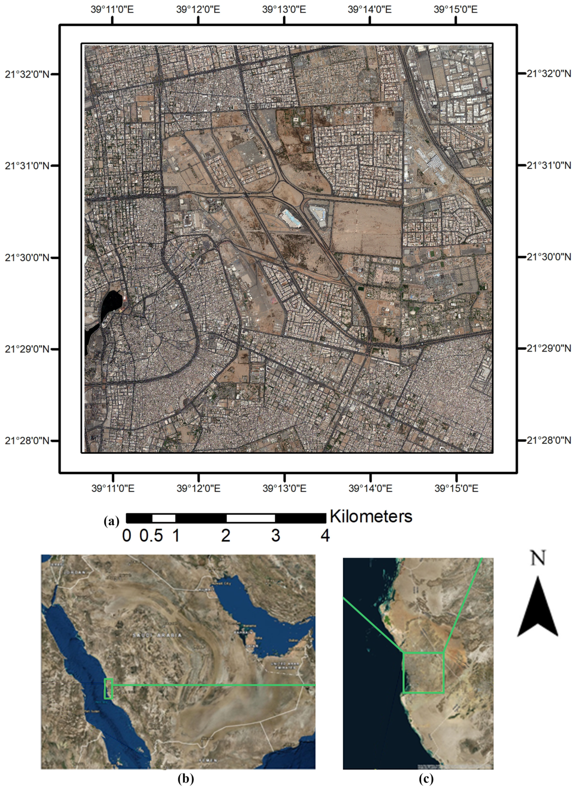
2.1. Area of Study
2.2. Dataset
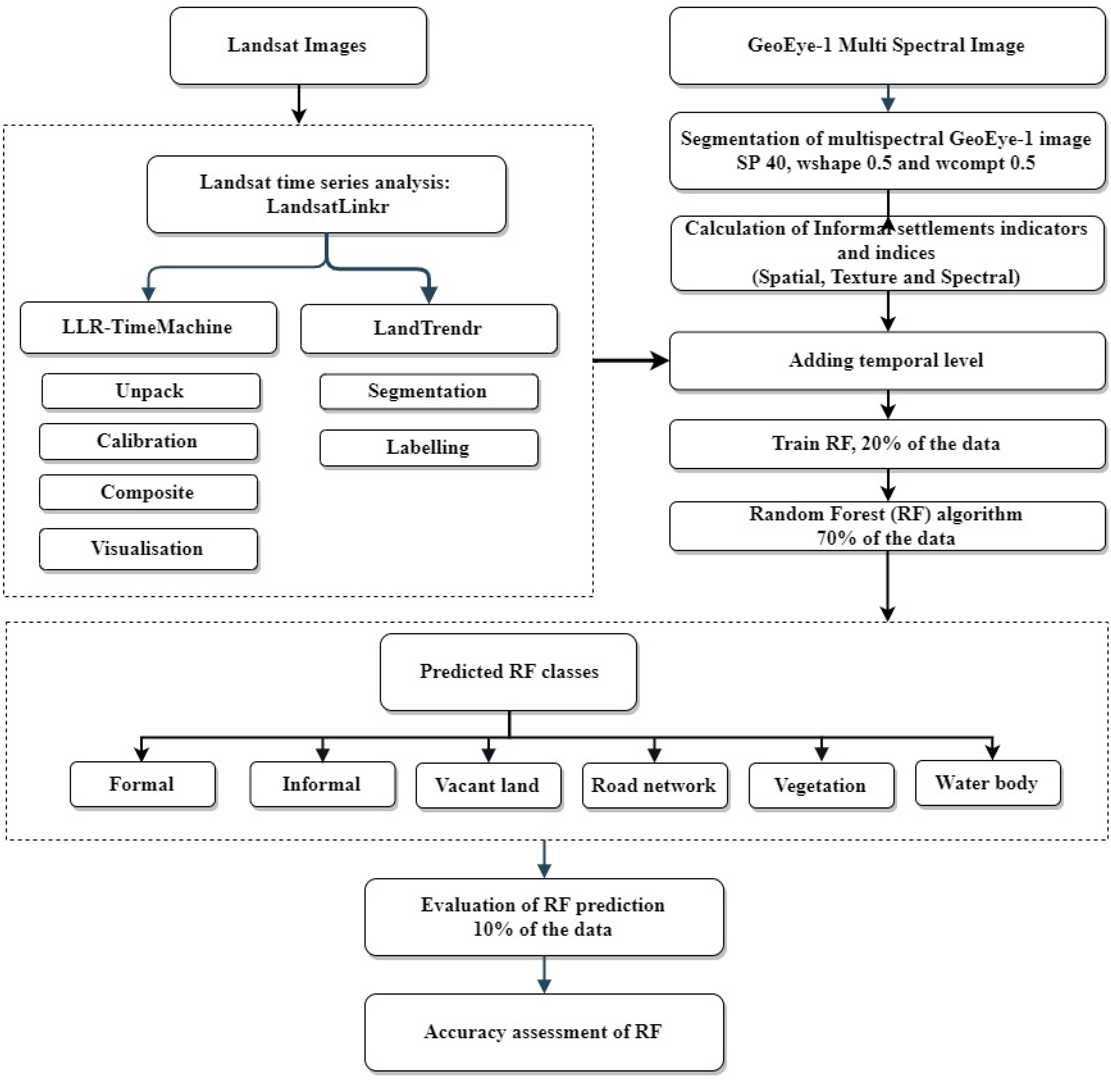
3. Methodology
3.1. Time-Series Analysis (TSA)
3.1.1. LandsatLinkr (LLR)-TimeMachine
3.1.2. LandTrendr
3.2. Object-Based Image Analysis (OBIA)
3.2.1. Segmentation
3.2.2. Object Attribution
3.3. Random Forest Classification
Training Data
3.4. Accuracy Assessment
4. Results
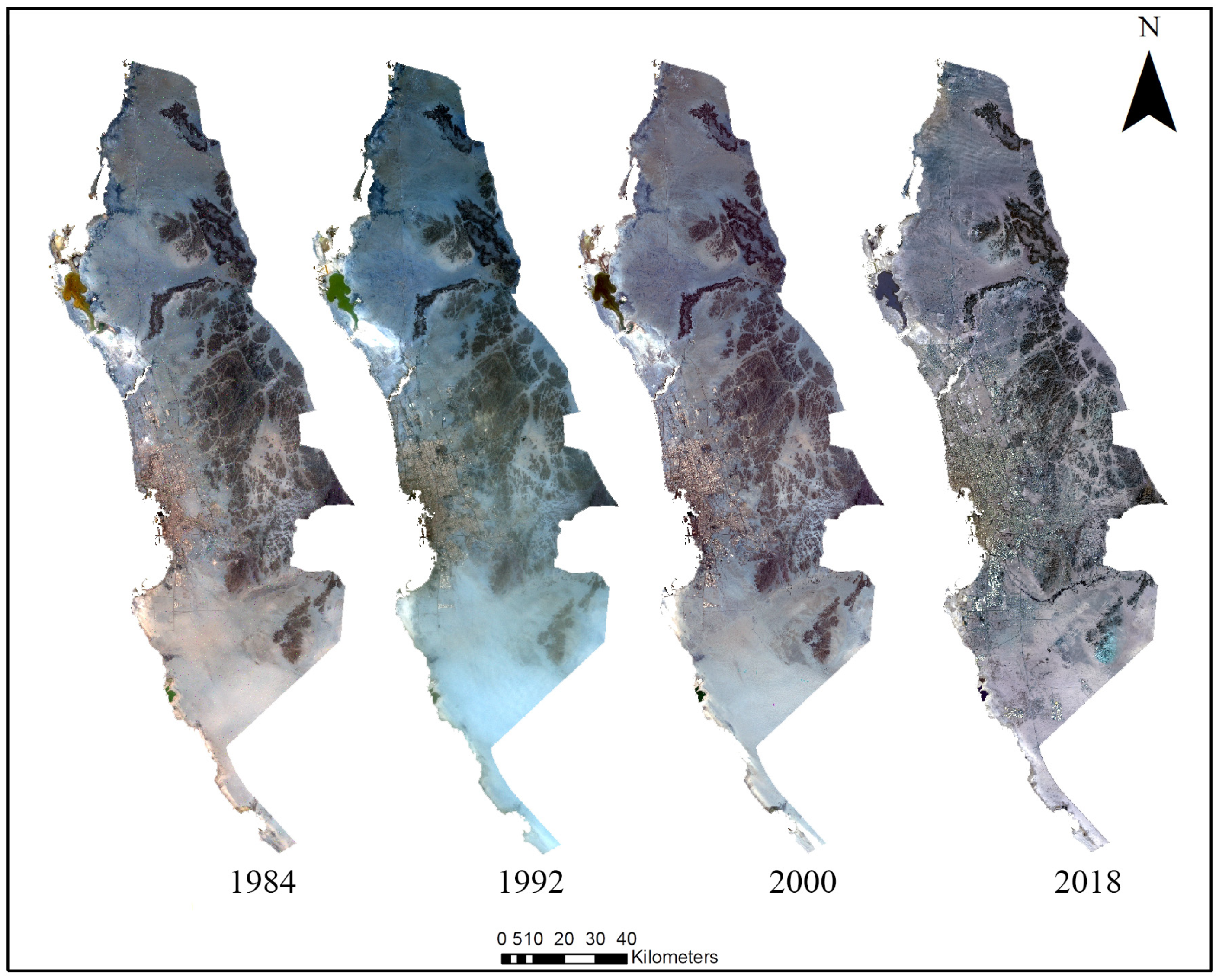
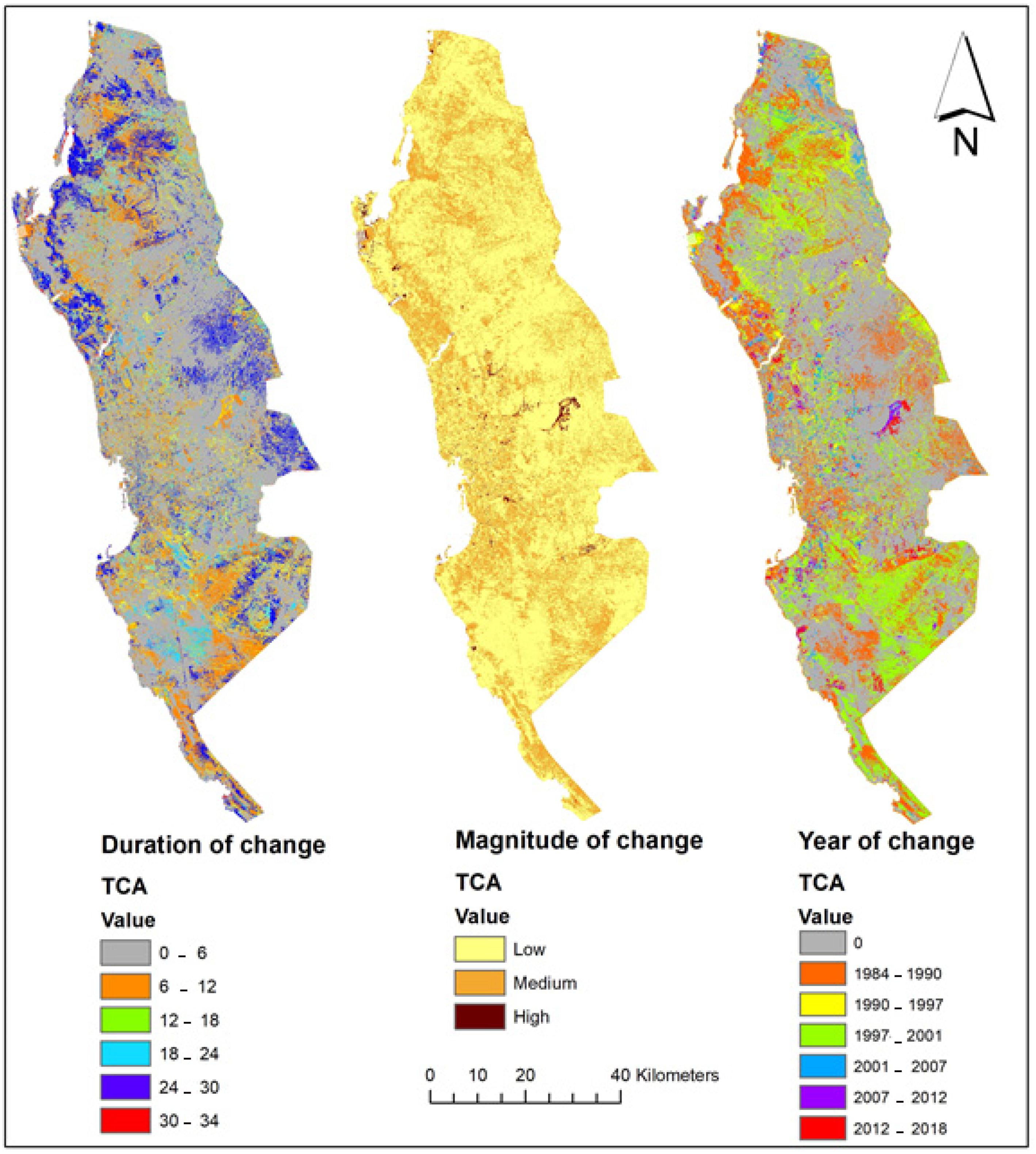
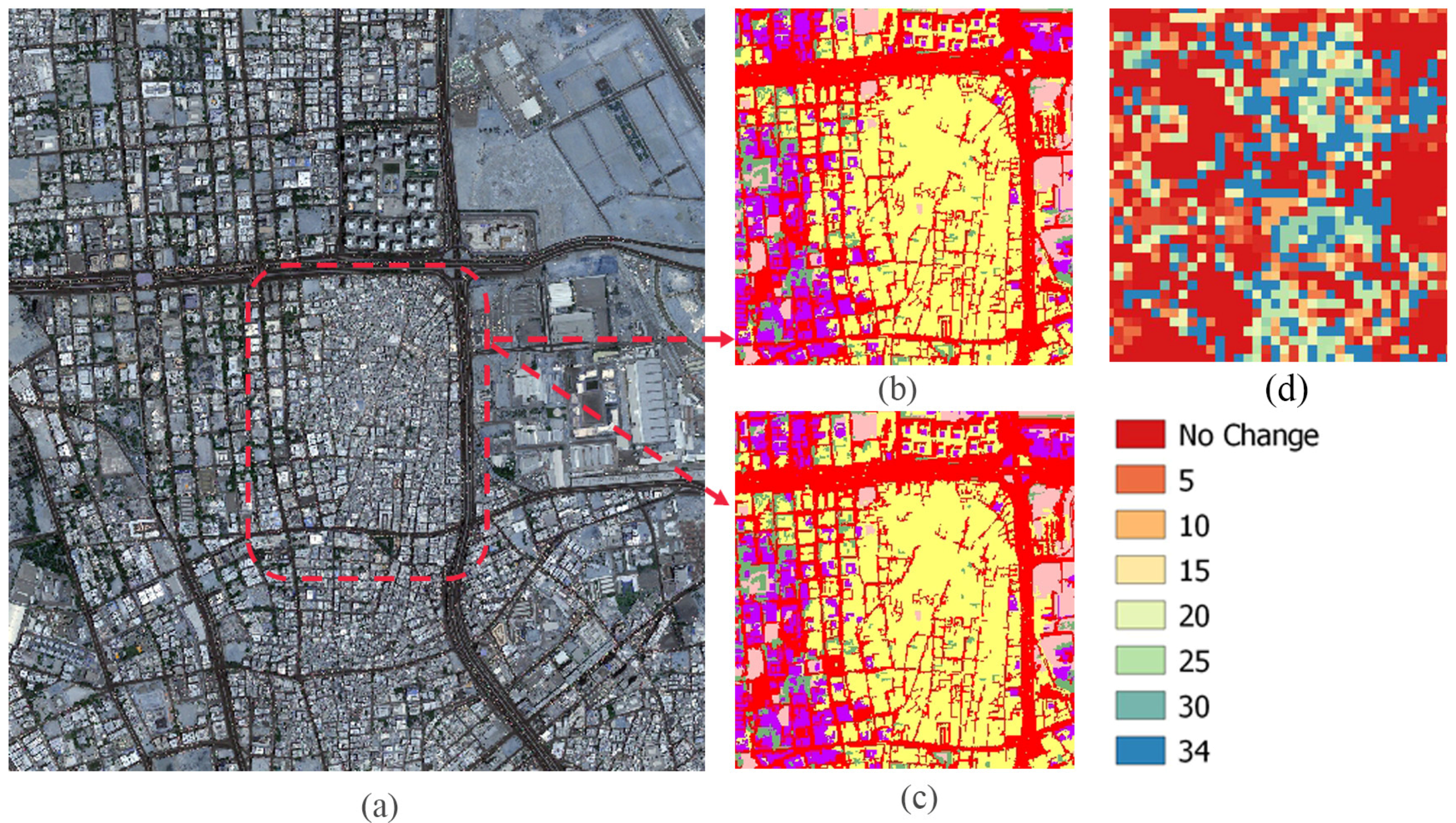
4.1. Time Series Analysis
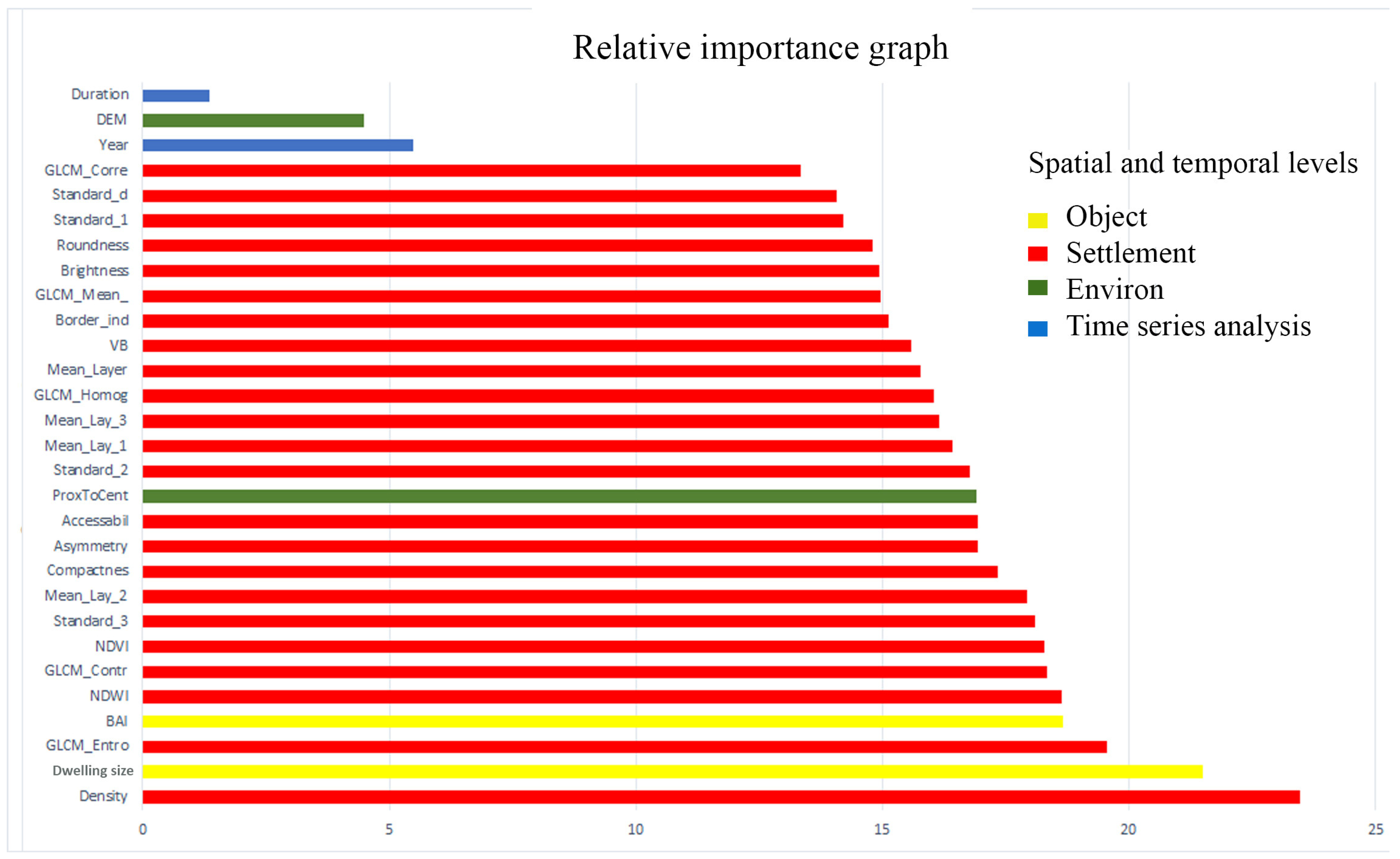
4.2. Classification Accuracy
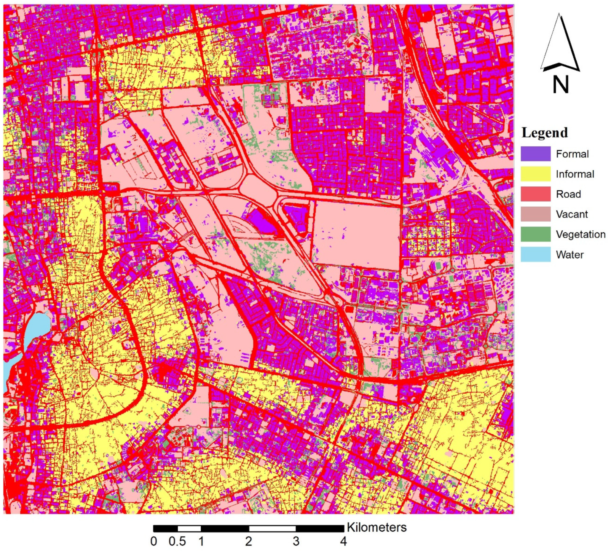
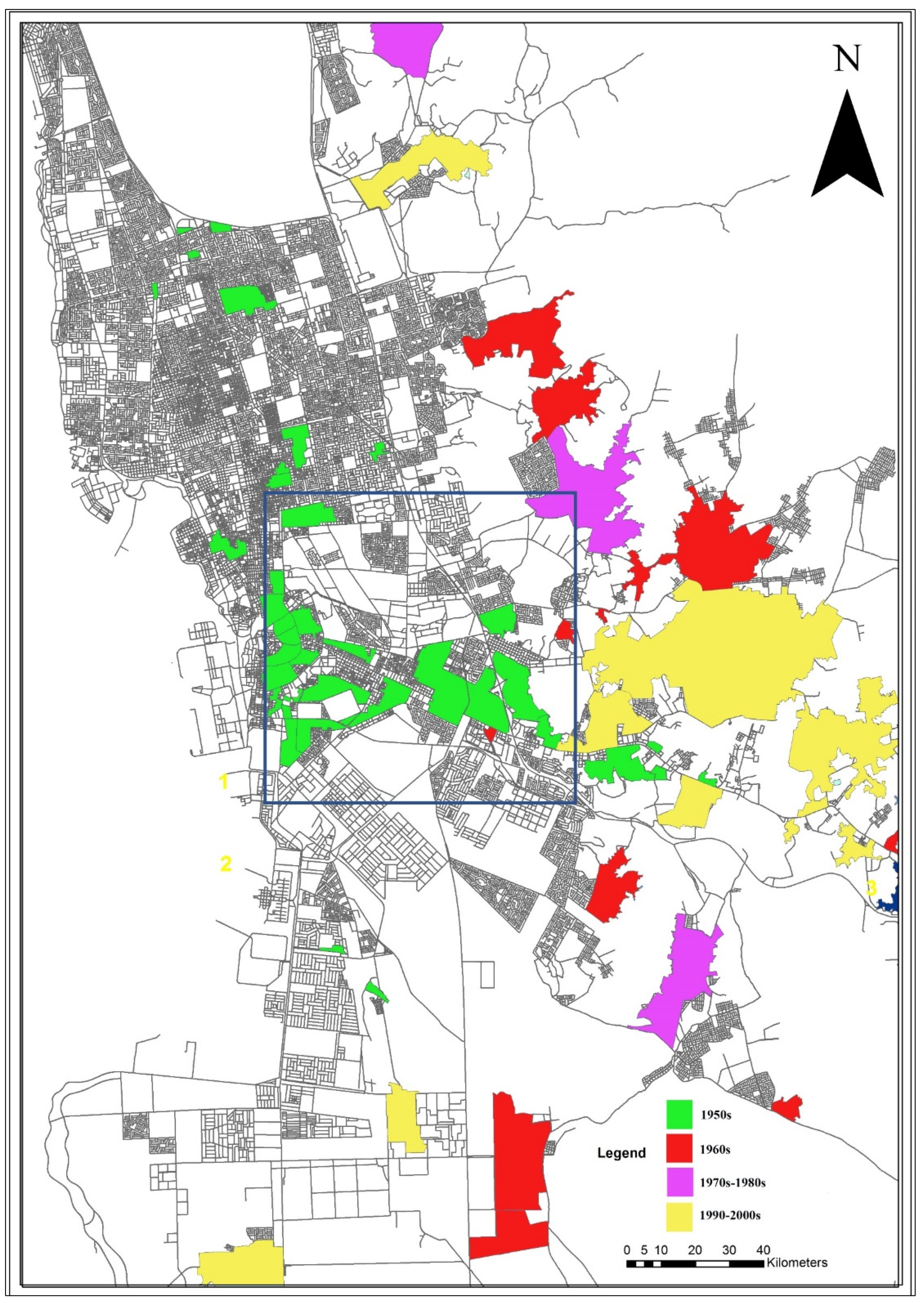
4.3. Temporal Analysis of Informal Settlements
5. Discussion
6. Conclusions
Author Contributions
Funding
Data Availability Statement
Acknowledgments
Conflicts of Interest
Appendix A

| Informal Settlements/Variable | Parameters | Description | Equation/Tool |
|---|---|---|---|
| * Built up area | Built up area index (BAI) | BAI is used to measure Built-up area. | BAI = (B1 − B4)/(B1 + B4) |
| * Dwelling size | Area | The number of pixels forming an image object. Mean dwelling sizes between <50 m2 and 380 m2 classified as informal settlements. | Object feature in eCognition |
| * vegetation | Normalised Difference Vegetation Index (NDVI) | NDVI is used to measure vegetation. | NDVI = (B4 − B3)/(B4 + B3) |
| * Lacunarity of housing structures | Visible brightness (VB) | The mean intensity of all the image bands for an image object. | VB = (B1 + B2 + B3)/3 |
| * Road segment type and materials | Normalised difference water index (NDWI) | NDWI: An index developed to distinguish tarred roads from other classes. | NDWI = (B2 − B4)/(B2 + B4) |
| * Texture measures | Grey-level co-occurrence matrix (GLCM) | GLCM entropy | Object feature in eCognition |
| GLCM homogeneity | |||
| GLCM contrast | |||
| GLCM correlation | |||
| GLCM mean. | |||
| Road accessibility | Accessibility | Based on road elongation and the regularity of road segments. Roads not easily accessible, a higher proportion of dead-ends (dangles) and fewer intersecting nodes. | Spatial analysis in ArcGIS |
| Consistency of housing orientation | Asymmetry | This indicates simplicity of shape. In the computer vision literature, the angles and lengths of line segments exhibit greater angular variability and shorter lengths in informal settlements. | Object feature in eCognition |
| Dwelling shape | Shape | The relative length of an image object, compared to a regular polygon. | Area of the segment/area of the minimum bounding rectangle of the segment. |
| Building density (dwelling separation) | Density | Lower nearest-neighbour distance using centroid of dwelling polygons. Density is calculated based on the image object that contains the current candidate pixel. This allows the smoothing of the border of the image object without taking neighbouring image objects into account. | Object feature in eCognition |
| Proximity to hazards | Digital elevation model (DEM) | Only flood hazards were considered. | Spatial analysis in ArcGIS |
| Geomorphology of terrain | Digital elevation model (DEM) | Settlements built on relatively flat surfaces. | Object feature in eCognition |
| Proximity to city centre and social services | ProxToCent | Network analysis of distance to city services, market area or city centre and healthcare facilities. Greater distances expected. | Spatial analysis in ArcGIS |
Appendix B
| Run_Name | Refpoints |
|---|---|
| base_index | TCA, TCB, TCG, TCW |
| background_val | 0 |
| divisor | 1 |
| minneeded | 6 |
| kernelsize | 1 |
| pval | 0.05 |
| fix_doy_effect | 1 |
| max_segments | 7 |
| recovery_threshold | 1 |
| skipfactor | 1 |
| desawtooth_val | 1 |
| distweightfactor | 2 |
| vertexcountovershoot | 3 |
| bestmodelproportion | 0.75 |
| mask_image | na |
| ulx | na |
| uly | na |
| lrx | na |
| lry | na |
References
- Kuffer, M.; Pfeffer, K.; Sliuzas, R.; Baud, I. Extraction of Slum Areas from VHR Imagery Using GLCM Variance. IEEE J. Sel. Top. Appl. Earth Obs. Remote Sens. 2016, 9, 1830–1840. [Google Scholar] [CrossRef]
- Mitchell, D.; Enemark, S.; van der Molen, P. Climate resilient urban development: Why responsible land governance is important. Land Use Policy 2015, 48, 190–198. [Google Scholar] [CrossRef]
- Jones, P. Formalizing the Informal: Understanding the Position of Informal Settlements and Slums in Sustainable Urbanization Policies and Strategies in Bandung, Indonesia. Sustainability 2017, 9, 1436. [Google Scholar] [CrossRef] [Green Version]
- Kuffer, M.; Pfeffer, K.; Sliuzas, R. Slums from Space—15 Years of Slum Mapping Using Remote Sensing. Remote Sens. 2016, 8, 455. [Google Scholar] [CrossRef] [Green Version]
- Abascal, A.; Rothwell, N.; Shonowo, A.; Thomson, D.; Elias, P.; Yeboah, G.; Kuffer, M. Domains of deprivation framework” for mapping slums, informal settlements, and other deprived areas in LMICs to improve urban planning and policy: A scoping review. Comput. Environ. Urban Syst. 2022, 93, 101770. [Google Scholar] [CrossRef]
- UN-Habitat. Transforming Our World: The 2030 Agenda for Sustainable Development; UN-Habitat: New York, NY, USA, 2015. [Google Scholar]
- United Nations. Slums of the World: The Face of Urban Poverty in the New Millennium; UN-Habitat: Nairobi, Kenya, 2003. [Google Scholar]
- Chakraborty, A.; Wilson, B.; Sarraf, S.; Jana, A. Open data for informal settlements: Toward a user’s guide for urban managers and planners. J. Urban Manag. 2015, 4, 74–91. [Google Scholar] [CrossRef] [Green Version]
- Dadras, M.; Shafri, H.Z.M.; Ahmad, N.; Pradhan, B.; Safarpour, S. Spatio-temporal analysis of urban growth from remote sensing data in Bandar Abbas city, Iran. Egypt. J. Remote Sens. Space Sci. 2015, 18, 35–52. [Google Scholar] [CrossRef] [Green Version]
- Belal, A.A.; Moghanm, F.S. Detecting urban growth using remote sensing and GIS techniques in Al Gharbiya governorate, Egypt. Egypt. J. Remote Sens. Space Sci. 2011, 14, 73–79. [Google Scholar] [CrossRef] [Green Version]
- Mohamed, E.S.; Saleh, A.M.; Belal, A.A. Sustainability indicators for agricultural land use based on GIS spatial modeling in North of Sinai-Egypt. Egypt. J. Remote Sens. Space Sci. 2014, 17, 1–15. [Google Scholar] [CrossRef] [Green Version]
- Song, X.-P.; Sexton, J.O.; Huang, C.; Channan, S.; Townshend, J.R. Characterizing the magnitude, timing and duration of urban growth from time series of Landsat-based estimates of impervious cover. Remote Sens. Environ. 2016, 175, 1–13. [Google Scholar] [CrossRef]
- Lu, H.; Liu, C.; Li, N.; Fu, X.; Li, L. Optimal segmentation scale selection and evaluation of cultivated land objects based on high-resolution remote sensing images with spectral and texture features. Environ. Sci. Pollut. Res. 2021, 28, 27067–27083. [Google Scholar] [CrossRef]
- Alganci, U.; Seker, D.Z.; Sertel, E.; Kaya, S. Spatio-temporal analysis of urbanization related land use/cover dynamics using satellite imagery: Case study antalya, Turkey. In Proceedings of the 33rd Asian Conference on Remote Sensing 2012, Melbourne, Australia, 25 August–1 September 2012; pp. 1111–1116. [Google Scholar]
- Stoica, I.-V.; Zamfir, D.; Vîrghileanu, M. Evaluating the Territorial Impact of Built-Up Area Expansion in the Surroundings of Bucharest (Romania) through a Multilevel Approach Based on Landsat Satellite Imagery. Remote Sens. 2021, 13, 3969. [Google Scholar] [CrossRef]
- Randazzo, G.; Italiano, F.; Micallef, A.; Tomasello, A.; Cassetti, F.P.; Zammit, A.; D’Amico, S.; Saliba, O.; Cascio, M.; Cavallaro, F.; et al. WebGIS Implementation for Dynamic Mapping and Visualization of Coastal Geospatial Data: A Case Study of BESS Project. Appl. Sci. 2021, 11, 8233. [Google Scholar] [CrossRef]
- Healey, S.P.; Cohen, W.B.; Yang, Z.; Kenneth Brewer, C.; Brooks, E.B.; Gorelick, N.; Hernandez, A.J.; Huang, C.; Joseph Hughes, M.; Kennedy, R.E.; et al. Mapping forest change using stacked generalization: An ensemble approach. Remote Sens. Environ. 2018, 204, 717–728. [Google Scholar] [CrossRef]
- Liu, T.; Yang, X. Monitoring land changes in an urban area using satellite imagery, GIS and landscape metrics. Appl. Geogr. 2015, 56, 42–54. [Google Scholar] [CrossRef]
- Śleszyński, P.; Gibas, P.; Sudra, P. The Problem of Mismatch between the CORINE Land Cover Data Classification and the Development of Settlement in Poland. Remote Sens. 2020, 12, 2253. [Google Scholar] [CrossRef]
- Durieux, L.; Lagabrielle, E.; Nelson, A. A method for monitoring building construction in urban sprawl areas using object-based analysis of Spot 5 images and existing GIS data. ISPRS J. Photogramm. Remote Sens. 2008, 63, 399–408. [Google Scholar] [CrossRef]
- Hamedianfar, A.; Barakat, A.; Gibril, M. Large-scale urban mapping using integrated geographic object-based image analysis and artificial bee colony optimization from worldview-3 data. Int. J. Remote Sens. 2019, 40, 6796–6821. [Google Scholar] [CrossRef]
- Wang, Y.; Li, M. Urban Impervious Surface Detection From Remote Sensing Images: A review of the methods and challenges. IEEE Geosci. Remote Sens. Mag. 2019, 7, 64–93. [Google Scholar] [CrossRef]
- Kohli, D.; Sliuzas, R.; Stein, A. Urban slum detection using texture and spatial metrics derived from satellite imagery. J. Spat. Sci. 2016, 61, 405–426. [Google Scholar] [CrossRef] [Green Version]
- Kohli, D.; Warwadekar, P.; Kerle, N.; Sliuzas, R.; Stein, A. Transferability of Object-Oriented Image Analysis Methods for Slum Identification. Remote Sens. 2013, 5, 4209. [Google Scholar] [CrossRef] [Green Version]
- Fallatah, A.; Jones, S.; Mitchell, D.; Kohli, D. Mapping informal settlement indicators using object-oriented analysis in the Middle East. Int. J. Digit. Earth 2018, 12, 802–824. [Google Scholar] [CrossRef]
- Hofmann, P.; Strobl, J.; Blaschke, T.; Kux, H. Detecting informal settlements from QuickBird data in Rio de Janeiro using an object based approach. In Object-Based Image Analysis: Spatial Concepts for Knowledge-Driven Remote Sensing Applications; Blaschke, T., Lang, S., Hay, G.J., Eds.; Springer: Berlin/Heidelberg, Germany, 2008; pp. 531–553. [Google Scholar]
- Kuffer, M.; Wang, J.; Nagenborg, M.; Pfeffer, K.; Kohli, D.; Sliuzas, R.; Persello, C. The Scope of Earth-Observation to Improve the Consistency of the SDG Slum Indicator. ISPRS Int. J. Geo-Inf. 2018, 7, 428. [Google Scholar] [CrossRef] [Green Version]
- Fallatah, A.; Jones, S.; Mitchell, D. Object-based random forest classification for informal settlements identification in the Middle East: Jeddah a case study. Int. J. Remote Sens. 2020, 41, 4421–4445. [Google Scholar] [CrossRef]
- Chen, R.; Li, X.; Li, J. Object-Based Features for House Detection from RGB High-Resolution Images. Remote Sens. 2018, 10, 451. [Google Scholar] [CrossRef] [Green Version]
- Salas, E.; Boykin, K.; Valdez, R. Multispectral and Texture Feature Application in Image-Object Analysis of Summer Vegetation in Eastern Tajikistan Pamirs. Remote Sens. 2016, 8, 78. [Google Scholar] [CrossRef] [Green Version]
- Keshtkar, H.; Voigt, W.; Alizadeh, E. Land-cover classification and analysis of change using machine-learning classifiers and multi-temporal remote sensing imagery. Arab. J. Geosci. 2017, 10, 154. [Google Scholar] [CrossRef]
- Mellor, A.; Boukir, S.; Haywood, A.; Jones, S. Exploring issues of training data imbalance and mislabelling on random forest performance for large area land cover classification using the ensemble margin. ISPRS J. Photogramm. Remote Sens. 2015, 105, 155–168. [Google Scholar] [CrossRef]
- Kooistra, L.; Kuilder, E.T.; Mücher, C.A. Object-based random forest classification for mapping floodplain vegetation structure from nation-wide CIR AND LiDAR datasets. In Proceedings of the 2014 6th Workshop on Hyperspectral Image and Signal Processing: Evolution in Remote Sensing (WHISPERS), Lausanne, Switzerland, 24–27 June 2014; pp. 1–4. [Google Scholar]
- Förster, M.; Kleinschmit, B. Object-based classification of QuickBird data using ancillary information for the detection of forest types and NATURA 2000 habitats. In Object-Based Image Analysis: Spatial Concepts for Knowledge-Driven Remote Sensing Applications; Blaschke, T., Lang, S., Hay, G.J., Eds.; Springer: Berlin/Heidelberg, Germany, 2008; pp. 275–290. [Google Scholar]
- Cohen, W.B.; Yang, Z.; Healey, S.P.; Kennedy, R.E.; Gorelick, N. A LandTrendr multispectral ensemble for forest disturbance detection. Remote Sens. Environ. 2018, 205, 131–140. [Google Scholar] [CrossRef]
- Wulder, M.A.; Loveland, T.R.; Roy, D.P.; Crawford, C.J.; Masek, J.G.; Woodcock, C.E.; Allen, R.G.; Anderson, M.C.; Belward, A.S.; Cohen, W.B.; et al. Current status of Landsat program, science, and applications. Remote Sens. Environ. 2019, 225, 127–147. [Google Scholar] [CrossRef]
- Hislop, S.; Jones, S.; Soto-Berelov, M.; Skidmore, A.; Haywood, A.; Nguyen, T.H. A fusion approach to forest disturbance mapping using time series ensemble techniques. Remote Sens. Environ. 2019, 221, 188–197. [Google Scholar] [CrossRef]
- Kennedy, R.; Yang, Z.; Gorelick, N.; Braaten, J.; Cavalcante, L.; Cohen, W.; Healey, S. Implementation of the LandTrendr Algorithm on Google Earth Engine. Remote Sens. 2018, 10, 691. [Google Scholar] [CrossRef] [Green Version]
- Zhu, Z.; Wulder, M.A.; Roy, D.P.; Woodcock, C.E.; Hansen, M.C.; Radeloff, V.C.; Healey, S.P.; Schaaf, C.; Hostert, P.; Strobl, P.; et al. Benefits of the free and open Landsat data policy. Remote Sens. Environ. 2019, 224, 382–385. [Google Scholar] [CrossRef]
- Cohen, W.B.; Yang, Z.; Kennedy, R. Detecting trends in forest disturbance and recovery using yearly Landsat time series: 2. TimeSync—Tools for calibration and validation. Remote Sens. Environ. 2010, 114, 2911–2924. [Google Scholar] [CrossRef]
- Mboga, N.; Persello, C.; Bergado, J.R.; Stein, A. Detection of Informal Settlements from VHR Images Using Convolutional Neural Networks. Remote Sens. 2017, 9, 1106. [Google Scholar] [CrossRef] [Green Version]
- Nguyen, H.T.; Soto-Berelov, M.; Jones, S.D.; Haywood, A.; Hislop, S. Mapping forest disturbance and recovery for forest dynamics over large areas using Landsat time-series remote sensing. In Proceedings of the SPIE Remote Sensing, Warsaw, Poland, 2 November 2017; p. 11. [Google Scholar]
- Fu, P.; Weng, Q. A time series analysis of urbanization induced land use and land cover change and its impact on land surface temperature with Landsat imagery. Remote Sens. Environ. 2016, 175, 205–214. [Google Scholar] [CrossRef]
- Vieira, M.A.; Formaggio, A.R.; Rennó, C.D.; Atzberger, C.; Aguiar, D.A.; Mello, M.P. Object Based Image Analysis and Data Mining applied to a remotely sensed Landsat time-series to map sugarcane over large areas. Remote Sens. Environ. 2012, 123, 553–562. [Google Scholar] [CrossRef]
- Kohli, D.; Sliuzas, R.; Kerle, N.; Stein, A. An ontology of slums for image-based classification. Comput. Environ. Urban Syst. 2012, 36, 154–163. [Google Scholar] [CrossRef]
- Owen, K.K.; Wong, D.W. An approach to differentiate informal settlements using spectral, texture, geomorphology and road accessibility metrics. Appl. Geogr. 2013, 38, 107–118. [Google Scholar] [CrossRef]
- Kennedy, R.E.; Yang, Z.; Cohen, W.B. Detecting trends in forest disturbance and recovery using yearly Landsat time series: 1. LandTrendr—Temporal segmentation algorithms. Remote Sens. Environ. 2010, 114, 2897–2910. [Google Scholar] [CrossRef]
- Braaten, J.; Cohen, W.; Yang, Z. LandsatLinkr. Available online: http://doi.org/10.5281/zenodo.819474 (accessed on 30 May 2019).
- Zhu, Z.; Woodcock, C.E. Object-based cloud and cloud shadow detection in Landsat imagery. Remote Sens. Environ. 2012, 118, 83–94. [Google Scholar] [CrossRef]
- Haywood, A.; Verbesselt, J.; Baker, P. Mapping disturbance dynamics in wet sclerophyll forests using time series landsat. Int. Arch. Photogramm. Remote Sens. Spat. Inf. Sci. 2016, XLI-B8, 633–641. [Google Scholar] [CrossRef] [Green Version]
- White, J.C.; Wulder, M.A.; Hobart, G.W.; Luther, J.E.; Hermosilla, T.; Griffiths, P.; Coops, N.C.; Hall, R.J.; Hostert, P.; Dyk, A.; et al. Pixel-Based Image Compositing for Large-Area Dense Time Series Applications and Science. Can. J. Remote Sens. 2014, 40, 192–212. [Google Scholar] [CrossRef] [Green Version]
- Zhu, L.; Liu, X.; Wu, L.; Tang, Y.; Meng, Y. Long-Term Monitoring of Cropland Change near Dongting Lake, China, Using the LandTrendr Algorithm with Landsat Imagery. Remote Sens. 2019, 11, 1234. [Google Scholar] [CrossRef] [Green Version]
- USGS. Available online: https://www.usgs.gov/ (accessed on 30 April 2019).
- Barsi, J.; Schott, J.; Palluconi, F.; Hook, S. Validation of a Web-Based Atmospheric Correction Tool for Single Thermal Band Instruments; SPIE: Bellingham, WA, USA, 2005; Volume 5882. [Google Scholar]
- Haywood, A.; Mellor, A.; Stone, C. A strategic forest inventory for public land in Victoria, Australia. For. Ecol. Manag. 2016, 367, 86–96. [Google Scholar] [CrossRef]
- Crist, E.P. A TM Tasseled Cap equivalent transformation for reflectance factor data. Remote Sens. Environ. 1985, 17, 301–306. [Google Scholar] [CrossRef]
- Vogeler, J.C.; Braaten, J.D.; Slesak, R.A.; Falkowski, M.J. Extracting the full value of the Landsat archive: Inter-sensor harmonization for the mapping of Minnesota forest canopy cover (1973–2015). Remote Sens. Environ. 2018, 209, 363–374. [Google Scholar] [CrossRef]
- Aguilar, M.A.; Vicente, R.; Aguilar, F.J.; Fernández, A.; Saldaña, M.M. Optimizing object-based classification in urban environments using very high resolution geoeye-1 imagery. ISPRS Ann. Photogramm. Remote Sens. Spat. Inf. Sci. 2012, I-7, 99–104. [Google Scholar] [CrossRef] [Green Version]
- Benz, U.C.; Hofmann, P.; Willhauck, G.; Lingenfelder, I.; Heynen, M. Multi-resolution, object-oriented fuzzy analysis of remote sensing data for GIS-ready information. ISPRS J. Photogramm. Remote Sens. 2004, 58, 239–258. [Google Scholar] [CrossRef]
- Hofmann, P.; Lettmayer, P.; Blaschke, T.; Belgiu, M.; Wegenkittl, S.; Graf, R.; Lampoltshammer, T.J.; Andrejchenko, V. Towards a framework for agent-based image analysis of remote-sensing data. Int. J. Image Data Fusion 2015, 6, 115–137. [Google Scholar] [CrossRef] [Green Version]
- Nyandwi, E.; Koeva, M.; Kohli, D.; Bennett, R. Comparing Human versus Machine-Driven Cadastral Boundary Feature Extraction. Remote Sens. 2019, 11, 1662. [Google Scholar] [CrossRef] [Green Version]
- Kuffer, M.; Sliuzas, R.; Pfeffer, K.; Baud, I. The utility of the co-occurrence matrix to extract slum areas from VHR imagery. In Proceedings of the 2015 Joint Urban Remote Sensing Event, Lausanne, Switzerland, 30 March–1 April 2015. [Google Scholar]
- Haralick, R.M.; Shanmugam, K.; Dinstein, I. Textural Features for Image Classification. IEEE Trans. Syst. Man Cybern. 1973, SMC-3, 610–621. [Google Scholar] [CrossRef] [Green Version]
- de Leeuw, J.; Jia, H.; Yang, L.; Liu, X.; Schmidt, K.; Skidmore, A.K. Comparing accuracy assessments to infer superiority of image classification methods. Int. J. Remote Sens. 2006, 27, 223–232. [Google Scholar] [CrossRef]
- Breiman, L. Random Forests. Mach. Learn. 2001, 45, 5–32. [Google Scholar] [CrossRef] [Green Version]
- Ghorbanzadeh, O.; Valizadeh Kamran, K.; Blaschke, T.; Aryal, J.; Naboureh, A.; Einali, J.; Bian, J. Spatial Prediction of Wildfire Susceptibility Using Field Survey GPS Data and Machine Learning Approaches. Fire 2019, 2, 43. [Google Scholar] [CrossRef] [Green Version]
- Feng, Q.; Liu, J.; Gong, J. UAV Remote Sensing for Urban Vegetation Mapping Using Random Forest and Texture Analysis. Remote Sens. 2015, 7, 1074–1094. [Google Scholar] [CrossRef] [Green Version]
- Yuan, Y.; Hu, X. Random forest and objected-based classification for forest pest extraction from uav aerial imagery. Int. Arch. Photogramm. Remote Sens. Spat. Inf. Sci. 2016, XLI-B1, 1093–1098. [Google Scholar] [CrossRef] [Green Version]
- Mahabir, R.; Croitoru, A.; Crooks, A.T.; Agouris, P.; Stefanidis, A. A Critical Review of High and Very High-Resolution Remote Sensing Approaches for Detecting and Mapping Slums: Trends, Challenges and Emerging Opportunities. Urban Sci. 2018, 2, 8. [Google Scholar] [CrossRef] [Green Version]
- Blaschke, T. Object based image analysis for remote sensing. ISPRS J. Photogramm. Remote Sens. 2010, 65, 2–16. [Google Scholar] [CrossRef] [Green Version]
- Duro, D.C.; Franklin, S.E.; Dubé, M.G. A comparison of pixel-based and object-based image analysis with selected machine learning algorithms for the classification of agricultural landscapes using SPOT-5 HRG imagery. Remote Sens. Environ. 2012, 118, 259–272. [Google Scholar] [CrossRef]
- Duque, J.C.; Patino, J.E.; Betancourt, A. Exploring the Potential of Machine Learning for Automatic Slum Identification from VHR Imagery. Remote Sens. 2017, 9, 895. [Google Scholar] [CrossRef] [Green Version]
- Li, X.; Zhou, Y.; Zhu, Z.; Liang, L.; Yu, B.; Cao, W. Mapping annual urban dynamics (1985–2015) using time series of Landsat data. Remote Sens. Environ. 2018, 216, 674–683. [Google Scholar] [CrossRef]
- Medhi, A.; Kumar Saha, A. Rural Road Extraction using Object Based Image Analysis (OBIA): A case study from Assam, India. Adv. Cartogr. GIScience ICA 2019, 1, 1–8. [Google Scholar] [CrossRef] [Green Version]
- McFeeters, S.K. The use of the Normalized Difference Water Index (NDWI) in the delineation of open water features. Int. J. Remote Sens. 1996, 17, 1425–1432. [Google Scholar] [CrossRef]
- Zhao, X.; Yu, B.; Liu, Y.; Chen, Z.; Li, Q.; Wang, C.; Wu, J. Estimation of Poverty Using Random Forest Regression with Multi-Source Data: A Case Study in Bangladesh. Remote Sens. 2019, 11, 375. [Google Scholar] [CrossRef] [Green Version]
- Huang, B.; Zhao, B.; Song, Y. Urban land-use mapping using a deep convolutional neural network with high spatial resolution multispectral remote sensing imagery. Remote Sens. Environ. 2018, 214, 73–86. [Google Scholar] [CrossRef]
- Fu, Y.; Li, J.; Weng, Q.; Zheng, Q.; Li, L.; Dai, S.; Guo, B. Characterizing the spatial pattern of annual urban growth by using time series Landsat imagery. Sci. Total Environ. 2019, 666, 274–284. [Google Scholar] [CrossRef]


| Indicator | Description and Expected Informal Settlement Values | Level |
|---|---|---|
| Roofing extent of built-up area | The total area occupied covered by buildings. High densities are expected in urban settlements. | Object |
| Dwelling size | Mean dwelling size. Small dwellings (between <50 m2 and 380 m2) are expected in informal settlements. | Object |
| Vegetation extent | Total area covered by vegetation present. Low densities are expected in urban settlements. | Settlement |
| Lacunarity of housing structures | Measures heterogeneity or ‘gappiness’ of empty spaces (lacunae) between built-up structures. Low value expected. | Settlement |
| Road segment type and materials | Length and type of road segments. Less road elongation and fewer regular road segments are expected in informal settlements. | Settlement |
| Texture measures of built-up area | Measurement of the arrangement of colour and within an area. Less-structured and rapid changes expected in urban settlements. | Settlement |
| Road accessibility | Accessibility of roads for a range of vehicle types. Narrower roads less suitable for vehicular traffic; a higher proportion of dead-ends (dangles) and fewer intersecting nodes expected in informal settlements. | Settlement |
| Consistency of housing orientation | Consistency in orientation of the directions of line segments describing buildings. Low consistency expected in informal settlements. | Settlement |
| Dwelling shape | The height and shape of dwellings, including the simplicity of shape (four-sidedness). Simpler shapes in informal areas. | Settlement |
| Dwelling road setback | Distance of dwellings from roads. Precarious house placement and lack of road setbacks expected in urban settlements. | Settlement |
| Building density (dwelling separation) | Spacing between buildings. A lower separation is expected in informal settlements. | Settlement |
| Proximity to hazards | Proximity to hazourdous or potentially hazardous areas, including e-flood zones, hydrologic setbacks, landslide/earthquake, garbage mountains, point source pollution, airports, energy transmission lines, and major transportation. Informal settlements are more likely to be closer to these hazards. | Environ |
| Geomorphology of terrain | Properties (slope, elevation, aspect of the terrain, and soil type). Settlements built in gullies, ravines, steep slopes, and unstable soils are more likely to be informal. | Environ |
| Proximity to city centre and social services | Driving distance to the city centre and other civic services, such as markets and healthcare facilities. Greater distances expected for informal settlements. | Environ |
| Temporal development | The temporal properties of the most recent land cover change. Informat settlements are expected to occur rapidly and present a large difference in cover type. | Temporal |
| TM Bands (μm) | ETM + Bands (μm) |
|---|---|
| Band 1 (0.45–0.52) | Band 1 (0.45–0.515) |
| Band 2 (0.52–0.60) | Band 2 (0.525–0.605) |
| Band 3 (0.63–0.69) | Band 3 (0.63–0.69) |
| Band 4 (0.76–0.90) | Band 4 (0.75–0.90) |
| Band 5 (1.55–1.75) | Band 5 (1.55–1.75) |
| Band 6 (10.40–12.50) | Band 6 (10.40–12.50) |
| Band 7 (2.08–2.35) | Band 7 (2.09–2.35) |
| Compared Results | Mapping Accuracies | Difference/Improvement | |
|---|---|---|---|
| without TSA | with TSA | ||
| Formal | 92% | 94% | 2% |
| Informal | 95% | 97% | 2% |
| Road network | 89% | 90% | 1% |
| Vacant land | 94% | 93% | −1% |
| Vegetation | 95% | 96% | 1% |
| Water body | 100% | 100% | No change |
Publisher’s Note: MDPI stays neutral with regard to jurisdictional claims in published maps and institutional affiliations. |
© 2022 by the authors. Licensee MDPI, Basel, Switzerland. This article is an open access article distributed under the terms and conditions of the Creative Commons Attribution (CC BY) license (https://creativecommons.org/licenses/by/4.0/).
Share and Cite
Fallatah, A.; Jones, S.; Wallace, L.; Mitchell, D. Combining Object-Based Machine Learning with Long-Term Time-Series Analysis for Informal Settlement Identification. Remote Sens. 2022, 14, 1226. https://doi.org/10.3390/rs14051226
Fallatah A, Jones S, Wallace L, Mitchell D. Combining Object-Based Machine Learning with Long-Term Time-Series Analysis for Informal Settlement Identification. Remote Sensing. 2022; 14(5):1226. https://doi.org/10.3390/rs14051226
Chicago/Turabian StyleFallatah, Ahmad, Simon Jones, Luke Wallace, and David Mitchell. 2022. "Combining Object-Based Machine Learning with Long-Term Time-Series Analysis for Informal Settlement Identification" Remote Sensing 14, no. 5: 1226. https://doi.org/10.3390/rs14051226
APA StyleFallatah, A., Jones, S., Wallace, L., & Mitchell, D. (2022). Combining Object-Based Machine Learning with Long-Term Time-Series Analysis for Informal Settlement Identification. Remote Sensing, 14(5), 1226. https://doi.org/10.3390/rs14051226