
Towards Early Detection of Tropospheric Aerosol Layers Using Monitoring with Ceilometer, Photometer, and Air Mass Trajectories

 , , , ,
Abstract
:1. Introduction
2. Resources and Methodology
2.1. CHM15k Ceilometer Data
2.2. Photometer Data
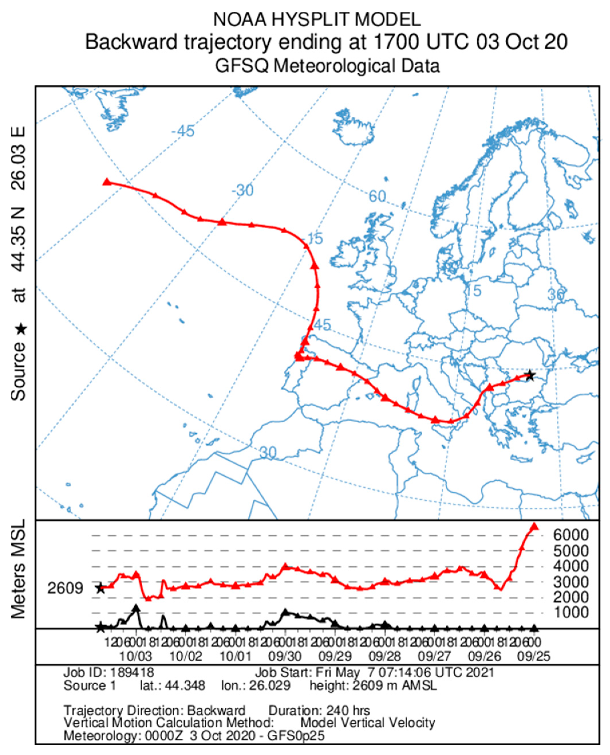
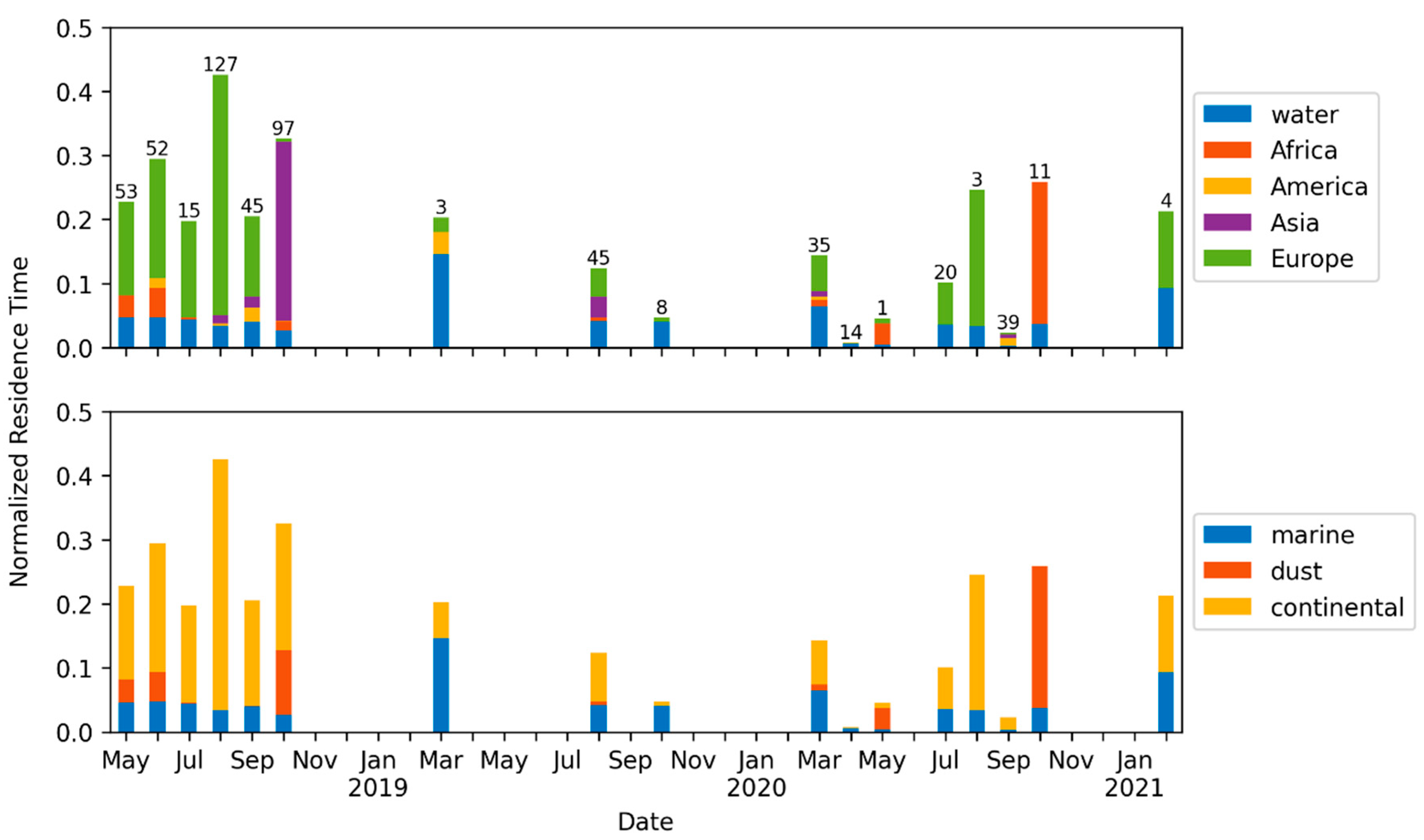
2.3. HYSPLIT Model
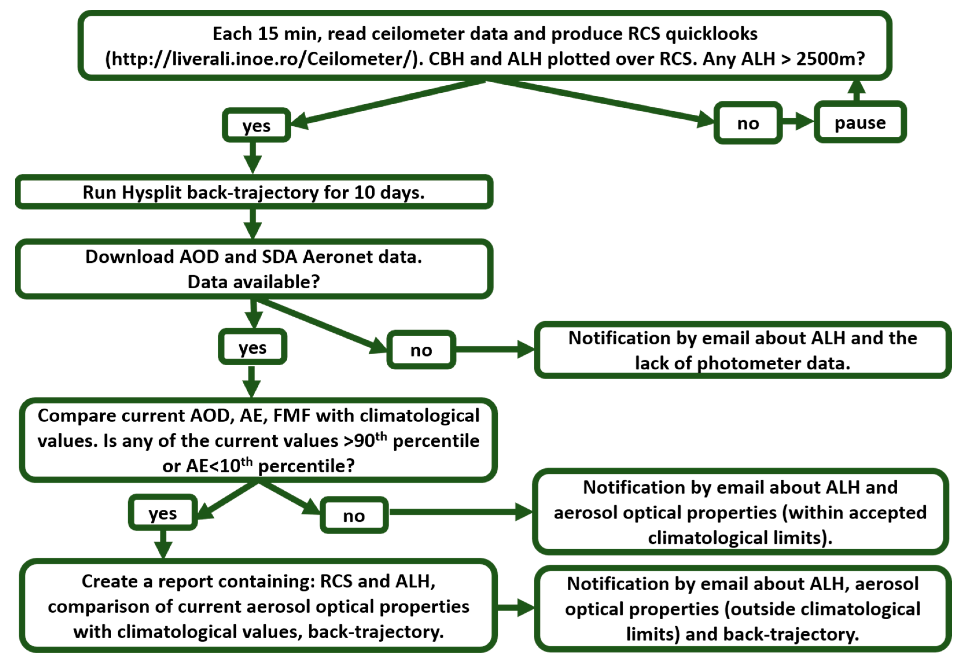
2.4. Methodology
- The early detection warning system works solely when photometer data are available (no precipitation and at least some cloud-free periods). In cases when cirrus clouds are present and the cloud screening data are not issued over the last 3 h, we do not perform the analysis.
- The AERONET data are released the earliest in about 1 h from the date of recording (timeliness). Consequently, the photometer data are not quite NRT. The photometer data used in the study covers 3 h interval from the time of the layer detection.
- ALH detected are limited up to ~4–5 km. As mentioned, the altitude of the pollution layers is taken as the top of the pollution. In a new version, once we implement our algorithm for layers identification, we will consider the middle of the layer.
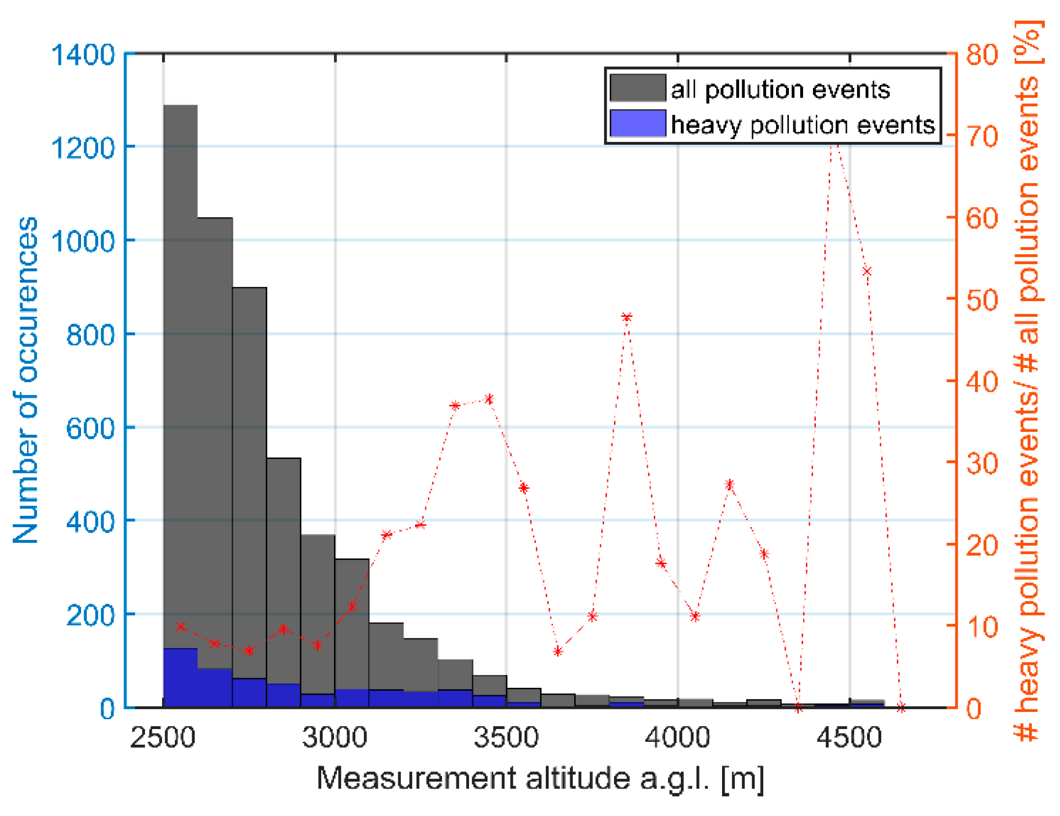
- The fixed threshold of the 2.5 km, in some cases is above the PBLH. This could result to missing some layers between the PBLH and 2.5 km. This issue is further discussed in Section 3.4, where we try to estimate the impact of the fixed height threshold at the number of possible layers that have not been identified by the algorithm.
- AERONET data are not available. Most of the cases occur because the weather was not favorable. However, sporadically we encountered also technical issues such as a failure in the transmission of the data from photometer towards Photons (Lille, France).
- The HYSPLIT back-trajectory could not be performed. In most cases, error messages indicate the lack of the meteorological fields.
- Local issues with internet disruptions.
- In rare cases, electrical power cut-offs that affect the operation of the ceilometer.
3. Results and Discussions
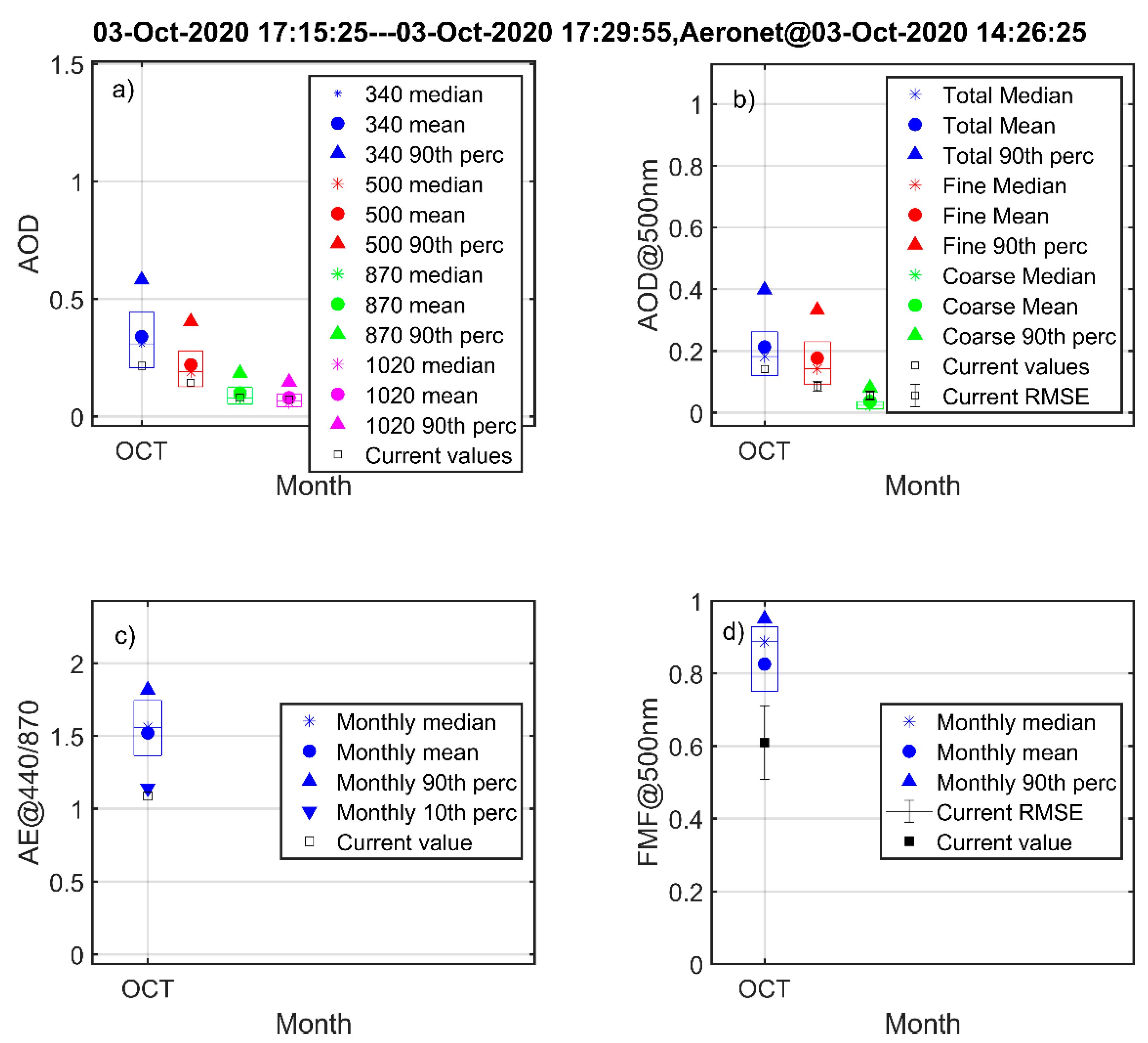
3.1. Example Report
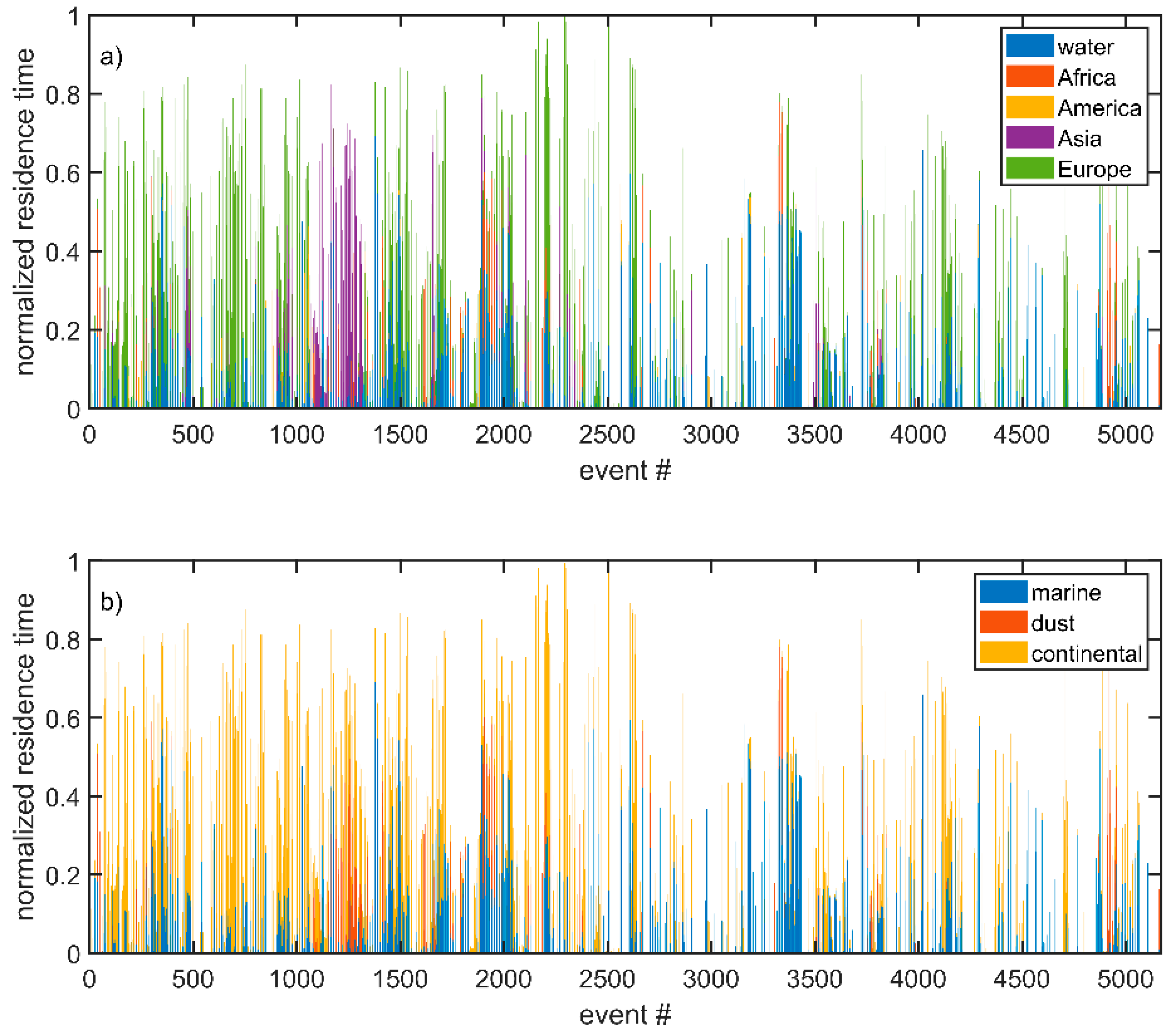
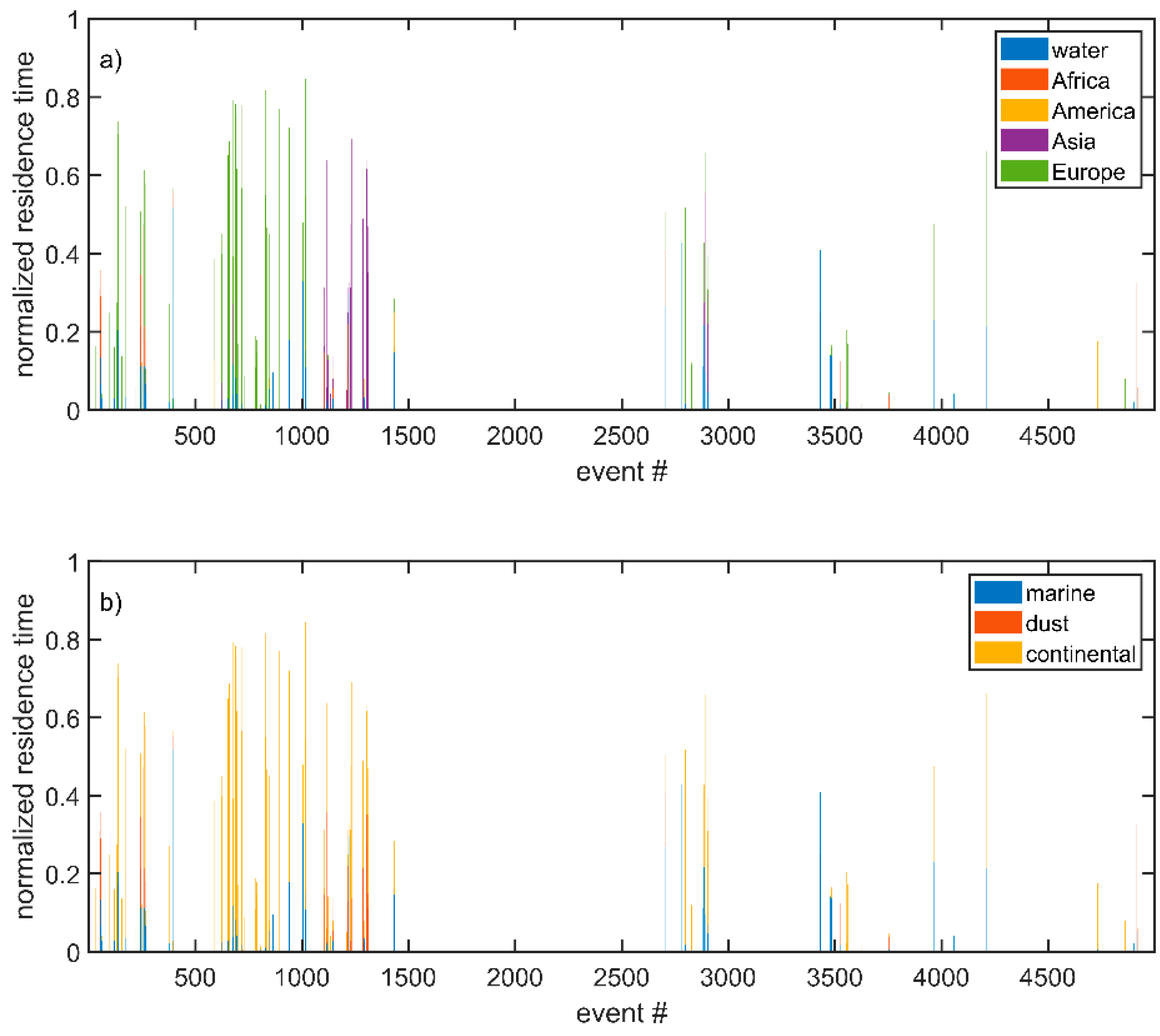
3.2. Some Statistics over the Colleted Data
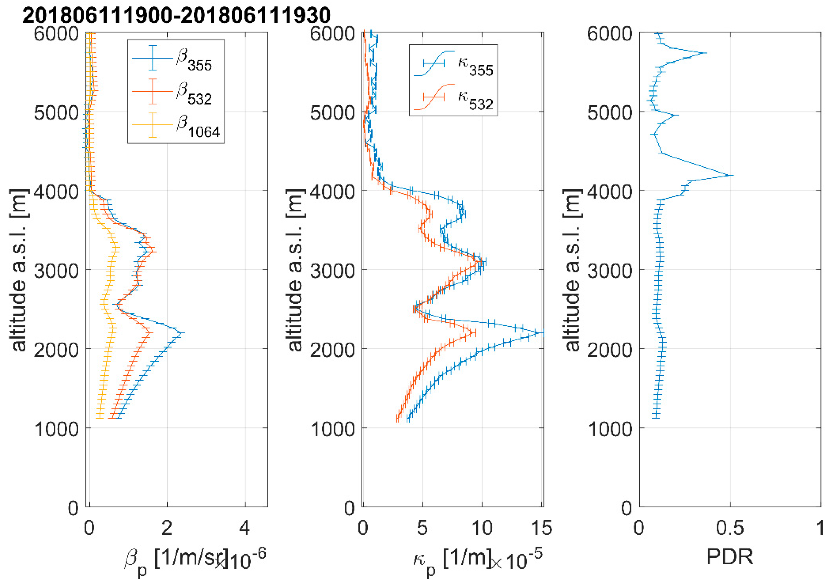
3.3. Case Study
3.4. Lessons Learnt over the Three-Year Testing Period
- -
- retrieval of the PBLH in NRT which allows the search of ALH above it, thus eliminating the constraint of 2500 m. Once the PBLH is estimated, the number of cases where ALH found in PBL will be eliminated;
- -
- retrieval of the ALH following the in-house developed algorithm allows to search for ALH above PBLH within FT, depending on the SNR of the ceilometer;
- -
- determination of the layers’ air mass source, following Radenz et al. [80];
- -
- update of the aerosol climatology of the optical properties derived from the photometer;
- -
- assessment of the contribution of the PBL and free troposphere in the total AOD.
4. Conclusions
Author Contributions
Funding
Acknowledgments
Conflicts of Interest
Abbreviations
| ACTRIS | Aerosol, Clouds and Trace Gases Research Infrastructure |
| AD-NET | Asian Dust and Aerosol Lidar Observation Network |
| AE | Ångström exponent |
| AERONET | Aerosol robotic network |
| a.g.l. | above ground level |
| ALH | Aerosol layer height |
| AOD: | Aerosol optical depth |
| a.s.l. | Above sea level |
| BAE | Backscatter Angstrom exponent |
| CBH | Cloud base height |
| CloudNet | Cloud Network |
| CMAOD | Coarse-mode aerosol optical depth |
| EAE | Extinction Angstrom exponent |
| EARLINET | European Aerosol Research Lidar Network |
| EEA | European Environment Agency |
| EPA | Environmental Protection Agency |
| E-PROFILE | EUMETNET Profiling Programme |
| EUMETNET | European National Meteorological Services |
| FMF | Fine-mode fraction |
| FMAOD | Fine-mode aerosol optical depth |
| FT | Free troposphere |
| GDAS | Global Data Assimilation System |
| GFS | Global Forecast System |
| HYSPLIT | Hybrid Single-Particle Lagrangian Integrated Trajectory model |
| INOE 2000 | National Institute of Research and Development for Optoelectronics |
| LALINET | Latin America Lidar Network |
| LR | Lidar ratio |
| MARS | Magurele Centre for Atmosphere and Radiation Studies |
| MERRA-2 | Modern-Era Retrospective Analysis for Research and Applications, Version 2 |
| MODIS | Moderate resolution imaging spectroradiometer |
| MPLNET | NASA Micro-Pulse Lidar Network |
| NDACC | Network for the Detection of Atmospheric Composition Change |
| NIR | Near-infrared region |
| NRT | Near real time |
| PBL | Planetary boundary layer |
| PBLH | Planetary boundary layer height |
| PDR | Particle linear depolarization ratio |
| PM | Particulate matter |
| RADO | Romanian atmospheric 3D Research Observatory |
| RCS | Range-corrected signal |
| RMSE | Root mean square error |
| ROLINET | Romanian LIdar NETwork |
| SDA | Spectral Deconvolution Algorithm |
| VAAC | Volcanic Ash Advisory Centre |
Appendix A
Appendix A.1. Notification about the Presence of ALH and the Absence of AERONET Data
20210128T065252 IIIrd ALH detected above 2.5 km a.g.l. (3.6462) over last 15 min, between 28-Jan-2021 06:47:19 and 28-Jan-2021 06:49:49UTC; no Aeronet data lev 1.5 in the last 3 h from 20210128T064719; keep an eye!
Appendix A.2. Notification about the Presence of ALH and the Values of the Optical Properties within the Climatological Limits
20210128T130207 IIIrd ALH detected above 2.5 km a.g.l. (3.876) over last 15 min, between 28-Jan-2021 12:58:50 and 28-Jan-2021 12:59:50UTC; Aeronet data lev 1.5 found in-20210127_20210128_Magurele_Inoe; within climatological limits; keep an eye!
Appendix A.3. Notification about the Presence of ALH and the Values of the Optical Properties outside the Climatological Limits
20210227T140206 IInd ALH detected above 2.5 km a.g.l. (2.6658) over last 15 min, between 27-Feb-2021 13:54:01 and 27-Feb-2021 13:59:31UTC; Aeronet data lev 1.5 found in-20210226_20210227_Magurele_Inoe; outside climatological limits; see file “\\172.16.1.15\Workspace\Documents\03-Stiintific\Analize\Mariana\CHM15k\CHM170137\PollutionEvents\20210227T135401_20210227T135931_IIndALH.pptx”; analyse results and take action!
Appendix B

Appendix C
References
- Pahlow, M.; Kleissl, J.; Parlange, M.B.; Ondov, J.M.; Harrison, D. Atmospheric boundary-layer strcture observed during a haze event due to forest-fire smoke. Bound. Layer Meteorol. 2005, 114, 53–70. [Google Scholar] [CrossRef]
- Sapkota, A.; Symons, J.M.; Kleissl, J.; Wang, L.; Parlange, M.B.; Ondov, J.; Breysse, P.N.; Diette, G.B.; Eggleston, P.A.; Buckley, T. Impact of the 2002 Canadian Forest Fires on Particulate Matter Air Quality in Baltimore City. Environ. Sci. Technol. 2002, 39, 24–32. [Google Scholar] [CrossRef] [PubMed] [Green Version]
- Amiridis, V.; Zeferos, C.; Kazadkis, S.; Gerasopoulos, E.; Eleftheratos, K.; Vrekoussis, M.; Stohl, A.; Mamouri, R.E.; Kokalis, P.; Papayannis, A.; et al. Impact of the 2009 Attica wild fires on the air quality in urban Athens. Atmos. Environ. 2012, 46, 536–544. [Google Scholar] [CrossRef]
- Alonso-Blanco, E.; Castro, A.; Calvo, A.I.; Pont, V.; Mallet, M.; Fraile, R. Wildfire smoke plumes transport under a subsidence inversion: Climate and health implications in a distant urban area. Sci. Total Environ. 2018, 619–620, 988–1002. [Google Scholar] [CrossRef]
- Clarkson, J.R.; Majewicz, E.J.E.; Mack, P. A re-evaluation of the 2010 quantitative understanding of the effects volcanic ash has on gas turbine engines. J. Aerosp. Eng. 2016, 230, 2274–2291. [Google Scholar] [CrossRef]
- Craig, H.; Wilson, T.; Stewart, C.; Outes, V.; Villarosa, G.; Baxter, P. Impacts to agriculture and critical infrastructure in Ar-gentina after ashfall from the 2011 eruption of the Cordón Caulle volcanic complex: An assessment of published damage and function thresholds. J. Appl. Volcanol. 2016, 5, 2–31. [Google Scholar] [CrossRef] [Green Version]
- Michailidis, K.; Koukouli, M.-E.; Siomos, N.; Balis, D.; Tuinder, O.; Tilstra, L.G.; Mona, L.; Pappalardo, G.; Bortoli, D. First validation of GOME-2/MetOp absorbing aerosol height using EARLINET lidar observations. Atmos. Chem. Phys. 2021, 21, 3193–3213. [Google Scholar] [CrossRef]
- Nemuc, A.; Boldeanu, M.; Dandocsi, A.; Adam, M.; Nicolae, V. Aerosol layer height from ground based active remote sensing and satellite ALH product of S5P/TROPOMI. In Proceedings of the European Lidar Conference 2021, Granada, Spain, 16–18 November 2021. [Google Scholar]
- Wiegner, M.; Madonna, F.; Binietoglou, I.; Forkel, R.; Gasteiger, R.; Geiß, A.; Pappalardo, G.; Schäfer, K.; Thomas, W. What is the benefit of ceilometers for aerosol remote sensing? An answer from EARLINET. Atmos. Meas. Tech. 2014, 7, 1979–1997. [Google Scholar] [CrossRef] [Green Version]
- Papagiannopoulos, N.; D’Amico, G.; Gialitaki, A.; Ajtai, N.; Alados-Arboledas, L.; Amodeo, A.; Amiridis, V.; Baars, H.; Balis, D.; Binietoglou, I.; et al. An EARLINET early warning system for atmospheric aerosol aviation hazards. Atmos. Chem. Phys. 2020, 20, 10775–10789. [Google Scholar] [CrossRef]
- Ratnam, M.V.; Prasad, P.; Raj, S.T.A.; Raman, M.R.; Basha, G. Changing patterns in aerosol vertical distribution over South and East Asia. Sci. Rep. 2021, 11, 308. [Google Scholar] [CrossRef]
- Pappalardo, G.; Amodeo, A.; Apituley, A.; Comeron, A.; Freudenthaler, V.; Linné, H.; Ansmann, A.; Bösenberg, J.; D’Amico, G.; Mattis, I.; et al. EARLINET: Towards an advanced sustainable European aerosol lidar network. Atmos. Meas. Tech. 2014, 7, 2389–2409. [Google Scholar] [CrossRef] [Green Version]
- Welton, E.J.; Voss, K.J.; Quinn, P.K.; Flatau, P.J.; Markowicz, K.; Campbell, J.R.; Spinhirne, J.D.; Gordon, H.R.; Johnson, J.E. Measurements of aerosol vertical profiles and optical properties during INDOEX 1999 using micro-pulse lidars. J. Geophys. Res. 2002, 107, 8019. [Google Scholar] [CrossRef]
- Lopes, F.J.S.; Silva, J.J.; Antuña Marrero, J.C.; Taha, G.; Landulfo, E. Synergetic Aerosol Layer Observation After the 2015 Calbuco Volcanic Eruption Event. Remote Sens. 2019, 11, 195. [Google Scholar] [CrossRef] [Green Version]
- Khaykin, S.M.; Godin-Beekmann, S.; Keckhut, P.; Hauchecorne, A.; Jumelet, J.; Vernier, J.-P.; Bourassa, A.; Degenstein, D.A.; Rieger, L.A.; Bingen, C.; et al. Variability and evolution of the midlatitude stratospheric aerosol budget from 22 years of ground-based lidar and satellite observations. Atmos. Chem. Phys. 2017, 17, 1829–1845. [Google Scholar] [CrossRef] [Green Version]
- Sugimoto, N.; Jin, Y.; Shimizu, A.; Nishizawa, T.; Yumimoto, K. Transport of Mineral Dust from Africa and Middle East to East Asia Observed with the Lidar Network (AD-Net). SOLA 2019, 15, 257–261. [Google Scholar] [CrossRef] [Green Version]
- Pappalardo, G.; Mona, L.; D’Amico, G.; Wandinger, U.; Adam, M.; Amodeo, A.; Ansmann, A.; Apituley, A.; Alados Arboledas, L.; Balis, D.; et al. Four-dimensional distribution of the 2010 Eyjafjallajökull volcanic cloud over Europe observed by EARLINET. Atmos. Chem. Phys. 2013, 13, 4429–4450. [Google Scholar] [CrossRef] [Green Version]
- Trickl, T.; Giehl, H.; Jäger, H.; Vogelmann, H. 35 yr of stratospheric aerosol measurements at Garmisch-Partenkirchen: From Fuego to Eyjafjallajökull, and beyond. Atmos. Chem. Phys. 2013, 13, 5205–5225. [Google Scholar] [CrossRef] [Green Version]
- Wang, X.; Boselli, A.; D’Avino, L.; Pisani, G.; Spinelli, N.; Amodeo, A.; Chaikovsky, A.; Wiegner, M.; Nickovic, S.; Papayannis, A.; et al. Volcanic dust characterization by EARLINET during Etna’s eruptions in 2001–2002. Atmos. Environ. 2008, 42, 893–905. [Google Scholar] [CrossRef]
- Sawamura, P.; Vernier, J.P.; Barnes, J.E.; Berkoff, T.A.; Welton, E.J.; Alados-Arboledas, L.; Navas-Guzmán, F.; Pappalardo, G.; Mona, L.; Madonna, F.; et al. Stratospheric AOD after the 2011 eruption of Nabro volcano measured by lidars over the Northern Hemisphere. Environ. Res. Lett. 2012, 7, 034013. [Google Scholar] [CrossRef] [Green Version]
- Ansmann, A.; Tesche, M.; Groß, S.; Freudenthaler, V.; Seifert, P.; Hiebsch, A.; Schmidt, J.; Wandinger, U.; Mattis, I.; Müller, D.; et al. The 16 April 2010 major volcanic ash plume over central Europe: EARLINET lidar and AERONET photometer observations at Leipzig and Munich, Germany. Geophys. Res. Lett. 2010, 37. [Google Scholar] [CrossRef] [Green Version]
- Adam, M.; Pahlow, M.; Kovalev, V.A.; Ondov, J.M.; Parlange, M.B.; Nair, N. Aerosol optical characterization by nephelometer and lidar: The Baltimore Supersite experiment during the Canadian forest fire smoke intrusion. J. Geophys. Res. 2004, 109. [Google Scholar] [CrossRef] [Green Version]
- Adam, M.; Nicolae, D.; Stachlewska, I.S.; Papayannis, A.; Balis, D. Biomass burning events measured by lidars in EARLINET—Part 1: Data analysis methodology. Atmos. Chem. Phys. 2020, 20, 13905–13927. [Google Scholar] [CrossRef]
- Hu, Q.; Goloub, P.; Veselovskii, I.; Bravo-Aranda, J.-A.; Popovici, I.E.; Podvin, T.; Haeffelin, M.; Lopatin, A.; Dubovik, O.; Pietras, C.; et al. Long-range transported Canadian smoke plumes in the lower stratosphere over northern France. Atmos. Chem. Phys. 2019, 19, 1173–1193. [Google Scholar] [CrossRef] [Green Version]
- Janicka, L.; Stachlewska, I.S.; Veselovskii, I.; Baars, H. Temporal variations in optical and microphysical properties of mineral dust and biomass burning aerosol derived from daytime Raman lidar observations over Warsaw, Poland. Atmos. Environ. 2017, 169, 162–174. [Google Scholar] [CrossRef]
- Müller, D.; Mattis, I.; Wandinger, U.; Ansmann, A.; Althausen, D.; Stohl, A. Raman lidar observations of aged Siberian and Canadian forest fire smoke in the free troposphere over Germany in 2003: Microphysical particle characterization. J. Geophys. Res. 2005, 110. [Google Scholar] [CrossRef]
- Nicolae, D.; Nemuc, A.; Müller, D.; Talianu, C.; Vasilescu, J.; Belegante, L.; Kolgotin, A. Characterization of fresh and aged biomass burning events using multiwavelength Raman lidar and mass spectrometry. J. Geophys. Res. Atmos. 2013, 118, 2956–2965. [Google Scholar] [CrossRef]
- Stachlewska, I.S.; Samson, M.; Zawadzka, O.; Harenda, K.M.; Janicka, L.; Poczta, P.; Szczepanik, D.; Heese, B.; Wang, D.; Borek, K.; et al. Modification of Local Urban Aerosol Properties by Long-Range Transport of Biomass Burning Aerosol. Remote Sens. 2018, 10, 412. [Google Scholar] [CrossRef] [Green Version]
- Veselovskii, I.; Whiteman, D.N.; Korenskiy, M.; Suvorina, A.; Kolgotin, A.; Lyapustin, A.; Wang, Y.; Chin, M.; Bian, H.; Kucsera, T.L.; et al. Characterization of forest fire smoke event near Washington, DC in summer 2013 with multi-wavelength lidar. Atmos. Chem. Phys. 2015, 15, 1647–1660. [Google Scholar] [CrossRef] [Green Version]
- Sicard, M.; Granados-Muñoz, M.J.; Alados-Arboledas, L.; Barragán, R.; Bedoya-Velásquez, A.E.; Benavent-Oltra, J.A.; Bortoli, D.; Comerón, A.; Córdoba-Jabonero, C.; Costa, M.J.; et al. Ground/space, passive/active remote sensing observations coupled with particle dispersion modelling to understand the inter-continental transport of wildfire smoke plumes. Remote Sens. Environ. 2019, 232, 111294. [Google Scholar] [CrossRef] [Green Version]
- Müller, D.; Ansmann, A.; Freudenthaler, V.; Kandler, K.; Toledano, C.; Hiebsch, A.; Gasteiger, J.; Esselborn, M.; Tesche, M.; Heese, B.; et al. Mineral dust observed with AERONET Sun photometer, Raman lidar, and in situ instruments during SAMUM 2006: Shape-dependent particle properties. J. Geophys. Res. 2010, 115. [Google Scholar] [CrossRef] [Green Version]
- Ansmann, A.; Rittmeister, F.; Engelmann, R.; Basart, S.; Jorba, O.; Spyrou, C.; Remy, S.; Skupin, A.; Baars, H.; Seifert, P.; et al. Profiling of Saharan dust from the Caribbean to western Africa –Part 2: Shipborne lidar measurements versus forecasts. Atmos. Chem. Phys. 2017, 17, 14987–15006. [Google Scholar] [CrossRef] [Green Version]
- Groß, S.; Freudenthaler, V.; Schepanski, K.; Toledano, C.; Schäfler, A.; Ansmann, A.; Weinzierl, B. Optical properties of long-range transported Saharan dust over Barbados as measured by dual-wavelength depolarization Raman lidar measurements. Atmos. Chem. Phys. 2015, 15, 11067–11080. [Google Scholar] [CrossRef] [Green Version]
- Mamouri, R.-E.; Ansmann, A.; Nisantzi, A.; Solomos, S.; Kallos, G.; Hadjimitsis, D.G. Extreme dust storm over the eastern Mediterranean in September 2015: Satellite, lidar, and surface observations in the Cyprus region. Atmos. Chem. Phys. 2016, 16, 13711–13724. [Google Scholar] [CrossRef] [Green Version]
- Binietoglou, I.; Basart, S.; Alados-Arboledas, L.; Amiridis, V.; Argyrouli, A.; Baars, H.; Baldasano, J.M.; Balis, D.; Belegante, L.; Bravo-Aranda, J.A.; et al. A methodology for investigating dust model performance using synergistic EARLINET/AERONET dust concentration re-trievals. Atmos. Meas. Tech. 2015, 8, 3577–3600. [Google Scholar] [CrossRef] [Green Version]
- Granados-Muñoz, M.J.; Bravo-Aranda, J.A.; Baumgardner, D.; Guerrero-Rascado, J.L.; Pérez-Ramírez, D.; Navas-Guzmán, F.; Veselovskii, I.; Lyamani, H.; Valenzuela, A.; Olmo, F.J.; et al. A comparative study of aerosol microphysical properties retrieved from ground-based remote sensing and aircraft in situ measurements during a Saharan dust event. Atmos. Meas. Tech. 2016, 9, 1113–1133. [Google Scholar] [CrossRef] [Green Version]
- Osborne, M.; Malavelle, F.F.; Adam, M.; Buxmann, J.; Sugier, J.; Marenco, F.; Haywood, J. Saharan dust and biomass burning aerosols during ex-hurricane Ophelia: Observations from the new UK lidar and sun-photometer Network. Atmos. Chem. Phys. 2019, 19, 3557–3578. [Google Scholar] [CrossRef] [Green Version]
- Vaughan, G.; Draude, A.P.; Ricketts, H.M.A.; Schultz, D.M.; Adam, M.; Sugier, J.; Wareing, D.P. Transport of Canadian forest fire smoke over the UK as observed by lidar. Atmos. Chem. Phys. 2018, 18, 11375–11388. [Google Scholar] [CrossRef] [Green Version]
- E-PROFILE. Available online: https://e-profile.eu/#/cm_profile (accessed on 20 May 2021).
- LUFFT. Available online: https://www.lufft.com/products/cloud-height-snow-depth-sensors-288/lufft-ceilometer-chm8k-2405/ (accessed on 20 May 2021).
- VAISALA. Available online: https://www.vaisala.com/en/products/instruments-sensors-and-other-measurement-devices/weather-stations-and-sensors/cl51 (accessed on 20 May 2021).
- Heese, B.; Flentje, H.; Althausen, D.; Ansmann, A.; Frey, S. Ceilometer lidar comparison: Backscatter coefficient retrieval and signal-to-noise ratio determination. Atmos. Meas. Tech. 2010, 3, 1763–1770. [Google Scholar] [CrossRef] [Green Version]
- O’Connor, E.J.; Illingworth, A.J.; Hogan, R. A technique for autocalibration of cloud lidar. J. Atmos. Ocean. Technol. 2004, 21, 777–786. [Google Scholar] [CrossRef]
- Holben, B.N.; Eck, T.F.; Slutsker, I.; Tanre, D.; Buis, J.P.; Setzer, A.; Vermote, E.; Reagan, J.A.; Kaufman, Y.J.; Nakajima, T.; et al. AERONET—A federated instrument network and data archive for aerosol characterization. Remote Sens. Environ. 1998, 66, 1–16. [Google Scholar] [CrossRef]
- Cazorla, A.; Casquero-Vera, J.A.; Román, R.; Guerrero-Rascado, J.L.; Toledano, C.; Cachorro, V.E.; Orza, J.A.G.; Cancillo, M.L.; Serrano, A.; Titos, G.; et al. Near-real-time processing of a ceilometer network assisted with sun-photometer data: Monitoring a dust outbreak over the Iberian Peninsula. Atmos. Chem. Phys. 2017, 17, 11861–11876. [Google Scholar] [CrossRef] [Green Version]
- CIMEL. Available online: https://www.cimel.fr/?instrument=sun-sky-lunar-multiband-photometer&lang=en (accessed on 20 May 2021).
- Kawai, K.; Nishio, Y.; Kai, K.; Noda, J.; Munkhjargal, E.; Shinoda, M.; Sugimoto, N.; Shimizu, A.; Davaanyam, E.; Batdorj, D. Ceilometer observation of a dust event in the Gobi Desert on 29−30 April 2015: Sudden arrival of a developed dust storm and trapping of dust within an inversion layer. SOLA 2019, 15, 52–56. [Google Scholar] [CrossRef] [Green Version]
- Marcos, C.R.; Gómez-Amo, J.L.; Peris, C.; Pedrós, R.; Utrillas, M.P.; Martínez-Lozano, J.A. Analysis of four years of ceilometer-derived aerosol backscatter profiles in a coastal site of the western Mediterranean. Atmos. Res. 2018, 213, 331–346. [Google Scholar] [CrossRef]
- Madonna, F.; Amato, F.; Vande Hey, J.; Pappalardo, G. Ceilometer aerosol profiling versus Raman lidar in the frame of the INTERACT campaign of ACTRIS. Atmos. Meas. Tech. 2015, 8, 2207–2223. [Google Scholar] [CrossRef] [Green Version]
- Stachlewska, I.S.; Piadlowski, M.; Migacz SSzkop, A.; Zielinska, A.J.; Swaczyna, P.L. Ceilometer Observations of the Boundary Layer over Warsaw, Poland. Acta Geophys. 2012, 60, 1386–1412. [Google Scholar] [CrossRef]
- Young, J.S.; Whiteman, C.D. Laser Ceilometer Investigation of Persistent Wintertime Cold-Air Pools in Utah’s Salt Lake Valley. J. Appl. Meteorol. Climatol. 2015, 54, 752–765. [Google Scholar] [CrossRef]
- Lotteraner, C.; Piringer, M. Mixing-Height Time Series from Operational Ceilometer Aerosol-Layer Heights. Bound. Layer Meteorol. 2016, 161, 265–287. [Google Scholar] [CrossRef] [Green Version]
- Lee, J.; Hong, J.-W.; Lee, K.; Hong, J.; Velasco, E.; Lim, Y.J.; Lee, J.B.; Nam, K.; Park, P. Ceilometer Monitoring of Boundary—Layer Height and Its Application in Evaluating the Dilution Effect on Air Pollution. Bound. Layer Meteorol. 2019, 172, 435–455. [Google Scholar] [CrossRef] [Green Version]
- Yang, Y.; Preißler, J.; Wiegner, M.; von Löwis, S.; Petersen, G.N.; Parks, M.M.; Finger, D.C. Monitoring Dust Events Using Doppler Lidar and Ceilometer in Iceland. Atmosphere 2020, 11, 1294. [Google Scholar] [CrossRef]
- Tsaknakis, G.; Papayannis, A.; Kokkalis, P.; Amiridis, A.; Kambezidis, H.D.; Mamouri, R.E.; Georgoussis, G.; Avdikos, G. Inter-comparison of lidar and ceilometer retrievals for aerosol and Planetary Boundary Layer profiling over Athens, Greece. Atmos. Meas. Tech. 2011, 4, 1261–1273. [Google Scholar] [CrossRef] [Green Version]
- Selvaratnam, V.; Ordóñez, C.; Adam, M. Comparison of Planetary Boundary Layer Heights from Jenoptik Ceilometers and the Unified Model; Met Office: Exeter, UK, 2015. [Google Scholar]
- Kotthaus, S.; Grimmond, C.S.B. Atmospheric boundary-layer characteristics from ceilometer measurements. Part 1: A new method to track mixed layer height and classify clouds. Q. J. R. Meteorol. Soc. 2018, 144, 1525–1538. [Google Scholar] [CrossRef] [Green Version]
- Marenco, F.; Kent, J.; Adam, M.; Buxmann, J.; Francis, P.; Haywood, J. Remote sensing of volcanic ash at the Met Office. In Proceedings of the The 27th International Laser Radar Conference (ILRC 27), New York, NY, USA, 5–10 July 2015; p. 07003. [Google Scholar]
- Georgoussis, G.; Adam, M.; Avdikos, G. Signal to Noise Ratio Estimations for a Volcanic ASH Detection Lidar. Case Study: The Met Office. In Proceedings of the The 27th International Laser Radar Conference (ILRC 27), New York, NY, USA, 5–10 July 2015; p. 07002. [Google Scholar]
- Adam, M.; Turp, M.; Horseman, A.; Ordóñez, C.; Buxmann, J.; Sugier, J. From operational ceilometer network to operational lidar network. In Proceedings of the The 27th International Laser Radar Conference (ILRC 27), New York, NY, USA, 5–10 July 2015; p. 27007. [Google Scholar]
- Adam, M.; Buxmann, J.; Freeman, N.; Horseman, A.; Salmon, C.; Sugier, J.; Bennett, R. The UK lidar-sunphotomter operational volcanic ash monitoring network. In Proceedings of the The 28th International Laser Radar Conference (ILRC 28), Bucharest, Romania, 25–30 June 2017; p. 09006. [Google Scholar]
- Haeffelin, M.; Laffineur, Q.; Bravo-Aranda, J.-A.; Drouin, M.-A.; Casquero-Vera, J.-A.; Dupont, J.-C.; De Backer, H. Radiation fog formation alerts using attenuated backscatter power from automatic lidars and ceilometers. Atmos. Meas. Tech. 2016, 9, 5347–5365. [Google Scholar] [CrossRef] [Green Version]
- Lopatin, A.; Dubovik, O.; Fuertes, D.; Stenchikov, G.; Lapyonok, T.; Veselovskii, I.; Wienhold, F.G.; Shevchenko, I.; Hu, Q.; Parajuli, S. Synergy processing of diverse ground-based remote sensing and in situ data using the GRASP algorithm: Applications to radiometer, lidar and radiosonde observations. Atmos. Meas. Tech. 2021, 14, 2575–2614. [Google Scholar] [CrossRef]
- Adam, M.; Fragkos, K.; Binietoglou, I. Automatic alert system for tropospheric particulate pollution monitoring. In Proceedings of the The 29th International Laser Radar Conference (ILRC 29), Hefei, China, 24–28 June 2019; p. 03004. [Google Scholar]
- Nicolae, D.; Vasilesescu, J.; Carstea, E.; Stebel, K.; Prata, F. Romanian Atmospheric Research 3D Observatory: Synergy of instruments. Rom. Rep. Phys. 2010, 62, 838–853. [Google Scholar]
- CEO-TERRA. Available online: http://ceo-terra.inoe.ro/index.php/laboratoare-noi/ (accessed on 20 May 2021).
- ACTRIS. Available online: https://actris.nilu.no/Content/?pageid=2c994933685948cba4e6e2dece91b19b (accessed on 20 May 2021).
- LIVERALI. Available online: http://liverali.inoe.ro/Ceilometer/ (accessed on 20 May 2021).
- Holben, B.N.; Tanre, D.; Smirnov, A.; Eck, T.F.; Slutsker, I.; Abuhassan, N.; Newcomb, W.W.; Schafer, J.S.; Chatenet, B.; Lavenu, F.; et al. An emerging ground-based aerosol climatology: Aerosol optical depth from AERONET. J. Geophys. Res. 2011, 106, 12067–12097. [Google Scholar] [CrossRef]
- O’Neill, N.T.; Eck, T.F.; Smirnov, A.; Holben, B.N.; Thulasiraman, S. Spectral discrimination of coarse and fine mode optical depth. J. Geophys. Res. 2003, 108. [Google Scholar] [CrossRef]
- Dubovik, O.; King, M.D. A flexible inversion algorithm for retrieval of aerosol optical properties from sun and sky radiance measurements. J. Geophys. Res. 2000, 105, 20673–20696. [Google Scholar] [CrossRef] [Green Version]
- Dubovik, O.; Sinyuk, A.; Lapyonok, T.; Holben, B.N.; Mishchenko, M.; Yang, P.; Eck, T.F.; Volten, H.; Noz, O.M.; Veihelmann, B.; et al. Application of spheroid models to account for aerosol particle nonspheric-ity in remote sensing of desert dust. J. Geophys. Res. 2006, 111. [Google Scholar] [CrossRef] [Green Version]
- Carstea, E.; Fragkos, E.; Siomos, N.; Antonescu, B.; Belegante, L. Columnar aerosol measurements in a continental southeastern Europe site: Climatology and trends. Theor. Appl. Climatol. 2019, 137, 3149–3159. [Google Scholar] [CrossRef]
- Giles, D.M.; Sinyuk, A.; Sorokin, M.G.; Schafer, J.S.; Smirnov, A.; Slutsker, I.; Eck, T.F.; Holben, B.N.; Lewis, J.R.; Campbell, J.R.; et al. Advancements in the Aerosol Robotic Network (AERONET) Version 3 database—Automated near-real-time quality control algorithm with improved cloud screening for Sun photometer aerosol optical depth (AOD) measurements. Atmos. Meas. Tech. 2019, 12, 169–209. [Google Scholar] [CrossRef] [Green Version]
- Stein, A.F.; Draxler, R.R.; Rolph, G.D.; Stunder, B.J.B.; Cohen, M.D.; Ngan, F. NOAA’s HYSPLIT Atmospheric Transport and Dispersion Modeling System. Bull. Amer. Meteor. Soc. 2015, 96, 2059–2077. [Google Scholar] [CrossRef]
- Timofte, A.; Belegante, L.; Cazacu, M.M.; Albina, B.; Talianu, C.; Gurlui, S. Study of planetary boundary layer height from LIDAR measurements and ALARO model. J. Optoelectron. Adv. Mat. 2015, 17, 911–917. [Google Scholar]
- Crosbie, E.; Sorooshian, A.; Monfared, N.A.; Shingler, T.; Esmaili, O. A Multi-Year Aerosol Characterization for the Greater Tehran Area Using Satellite, Surface, and Modeling Data. Atmosphere 2014, 5, 178–197. [Google Scholar] [CrossRef] [PubMed] [Green Version]
- Sullivan, R.C.; Levy, R.C.; Pryor, S.C. Spatiotemporal coherence of mean and extreme aerosol particle events over eastern North America as observed from satellite. Atmos. Environ. 2015, 112, 126–135. [Google Scholar] [CrossRef]
- Sullivan, R.C.; Levy, R.C.; da Silva, A.M.; Pryor, S.C. Developing and diagnosing climate change indicators of regional aerosol optical properties. Sci. Rep. 2017, 7, 18093. [Google Scholar] [CrossRef]
- Radenz, M.; Seifert, P.; Baars, H.; Floutsi, A.A.; Yin, Z.; Bühl, J. Automated time–height-resolved air mass source attribution for profiling remote sensing applications. Atmos. Chem. Phys. 2021, 21, 3015–3033. [Google Scholar] [CrossRef]
- Georgoulias, A.K.; Alexandri, G.; Kourtidis, K.A.; Lelieveld, J.; Zanis, P.; Pöschl, U.; Levy, R.; Amiridis, V.; Marinou, E.; Tsikerdekis, A. Spatiotemporal variability and contribution of different aerosol types to the aerosol optical depth over the Eastern Mediterranean. Atmos. Chem. Phys. 2016, 16, 13853–13884. [Google Scholar] [CrossRef] [Green Version]
- Grigoras, G.; Mocioaca, G. Air quality assessment in Craiova urban area. Rom. Rep. Phys. 2012, 64, 768–787. [Google Scholar]
- Mihai, L.; Stefan, S. Temporal variation of aerosol optical properties at Magurele, Romania. J. Atmos. Ocean. Technol. 2011, 68, 1307–1316. [Google Scholar] [CrossRef]
- Fragkos, K.; Antonescu, B.; Giles, D.M.; Ene, D.; Boldeanu, M.; Efstathiou, G.A.; Belegante, L.; Nicolae, D. Assessment of the total precipitable water from a sun photometer, microwave radiometer and radiosondes at a continental site in southeastern Europe. Atmos. Meas. Tech. 2019, 12, 1979–1997. [Google Scholar] [CrossRef] [Green Version]
- Toanca, F.; Stefan, S.; Labzovskii, L.; Belegante, L.; Andrei, S.; Nicolae, D. Study of fog events using remote sensing data. Rom. Rep. Phys. 2017, 69, 703. [Google Scholar]
- Gelaro, R.; McCarty, W.; Suárez, M.J.; Todling, R.; Molod, A.; Takacs, L.; Randles, C.; Darmenov, A.; Bosilovich, M.G.; Reichle, R.; et al. The Modern-Era Retrospective Analysis for Research and Applications, Version 2 (MERRA-2). J. Clim. 2017, 30, 5419–5454. [Google Scholar] [CrossRef] [PubMed]
- Groß, S.; Esselborn, M.; Weinzierl, B.; Wirth, M.; Fix, A.; Petzold, A. Aerosol classification by airborne high spectral resolution lidar observations. Atmos. Chem. Phys. 2013, 13, 2487–2505. [Google Scholar] [CrossRef] [Green Version]
- Papayannis, A.; Amiridis, A.; Mona, L.; Tsaknakis, G.; Balis, D.; Bösenberg, J.; Chaikovski, A.; De Tomasi, F.; Grigorov, I.; Mattis, I.; et al. Systematic lidar observations of Saharan dust over Europe in the frame of EARLINET (2000–2002). J. Geophys. Res. 2008, 113. [Google Scholar] [CrossRef] [Green Version]
- Nicolae, D.; Vasilescu, J.; Talianu, C.; Binietoglou, I.; Nicolae, V.; Andrei, S.; Antonescu, B. A neural network aerosol-typing algorithm based on lidar data. Atmos. Chem. Phys. 2018, 18, 14511–14537. [Google Scholar] [CrossRef] [Green Version]
- Wang, D.; Stachlewska, I.S.; Song, X.; Heese, B.; Nemuc, A. Variability of the Boundary Layer Over an Urban Continental Site Based on 10 Years of Active Remote Sensing Observations in Warsaw. Remote Sens. 2020, 12, 340. [Google Scholar] [CrossRef] [Green Version]


| Variable | Wavelength [nm] |
|---|---|
| AOD > 90th percentile | 340, 500, 870, 1020 |
| AE < 10th percentile or AE > 90th percentile | 340/870 |
| FMAOD > 90th percentile CMAOD > 90th percentile | 500 |
| FMF > 90th percentile | 500 |
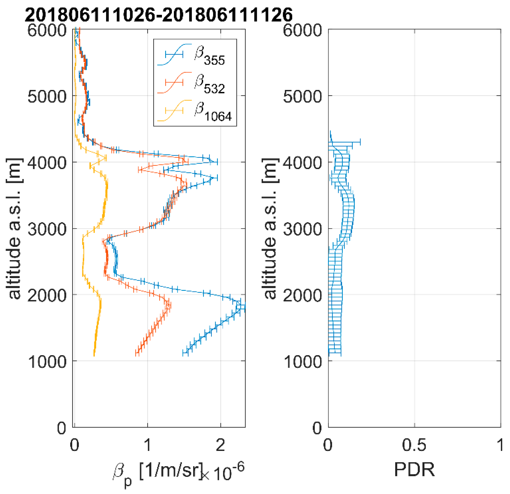
| Optical Property/ Measurement Time | PDR [%] | BAE 355/532 | BAE 532/1064 | LR355 [sr] | LR532 [sr] | EAE |
|---|---|---|---|---|---|---|
| 10:26–11:26 | 14 ± 2 | 0.1 ± 0.41 | 0.95 ± 0.16 | |||
| 11:26–12:27 | 12 ± 2.3 | 0.29 ± 0.34 | 1.78 ± 0.19 | |||
| 12:27–13:27 | 15 ± 3.5 | 0.15 ± 0.42 | 1.67 ± 0.19 | |||
| 13:27–14:28 | 15.5 ± 3 | 0.03 ± 0.39 | 1.83 ± 0.22 | |||
| 14:28–14:47 | 18 ± 3.6 | 0.01 ± 0.3 | 1.9 ± 0.33 | |||
| 19:01–19:30 | 10.6 ± 0.6 | -0.04 ± 0.20 | 1.24 ± 0.06 | 65 ± 12 | 57 ± 12 | 0.34 ± 0.28 |
Publisher’s Note: MDPI stays neutral with regard to jurisdictional claims in published maps and institutional affiliations. |
© 2022 by the authors. Licensee MDPI, Basel, Switzerland. This article is an open access article distributed under the terms and conditions of the Creative Commons Attribution (CC BY) license (https://creativecommons.org/licenses/by/4.0/).
Share and Cite
Adam, M.; Fragkos, K.; Binietoglou, I.; Wang, D.; Stachlewska, I.S.; Belegante, L.; Nicolae, V. Towards Early Detection of Tropospheric Aerosol Layers Using Monitoring with Ceilometer, Photometer, and Air Mass Trajectories. Remote Sens. 2022, 14, 1217. https://doi.org/10.3390/rs14051217
Adam M, Fragkos K, Binietoglou I, Wang D, Stachlewska IS, Belegante L, Nicolae V. Towards Early Detection of Tropospheric Aerosol Layers Using Monitoring with Ceilometer, Photometer, and Air Mass Trajectories. Remote Sensing. 2022; 14(5):1217. https://doi.org/10.3390/rs14051217
Chicago/Turabian StyleAdam, Mariana, Konstantinos Fragkos, Ioannis Binietoglou, Dongxiang Wang, Iwona S. Stachlewska, Livio Belegante, and Victor Nicolae. 2022. "Towards Early Detection of Tropospheric Aerosol Layers Using Monitoring with Ceilometer, Photometer, and Air Mass Trajectories" Remote Sensing 14, no. 5: 1217. https://doi.org/10.3390/rs14051217
APA StyleAdam, M., Fragkos, K., Binietoglou, I., Wang, D., Stachlewska, I. S., Belegante, L., & Nicolae, V. (2022). Towards Early Detection of Tropospheric Aerosol Layers Using Monitoring with Ceilometer, Photometer, and Air Mass Trajectories. Remote Sensing, 14(5), 1217. https://doi.org/10.3390/rs14051217