Generating Terrain Data for Geomorphological Analysis by Integrating Topographical Features and Conditional Generative Adversarial Networks

Abstract

With the development of artificial intelligence techniques for geographical knowledge discovery, simulated terrain generation based on deep-learning algorithms has become one practical way to construct accurate terrain data. However, it is still necessary to discuss whether the simulated topographic data contain the characteristics of specific landforms and can support related geographical studies. Therefore, in this study, a deep learning-based model inspired by previous research is constructed to generate loess landform data. We analyzed the influence of inputting different topographic features on terrain generation and evaluated the similarity between the simulated and reference data. The results show that the deep learning-based model can generate simulated topographic data that include similar elevation and slope probability distributions to the reference data of the loess landform. In addition, the generated results may have inaccurate terrain details, which can be regarded as noise in some cases. This indicates that the selection of input features should be carefully considered. Finally, the simulated data can subsequently support landform and terrain research, especially with intelligence algorithms that require large sets of topographic data.

1. Introduction

Terrain is the fundamental object that significantly influences the geomorphic, hydrologic, and ecological processes of the Earth’s surface [1,2]. Various topographic characteristics carried by different surfaces provide information for landform classification, environmental evolution, terrain analysis, and hydrological analysis [3,4,5,6]. The digital elevation model (DEM) plays an important role in transferring geographical knowledge to computer-processable information [6]. It achieves a reliable way to represent the surface and supports the development of sophisticated techniques for geographical research [7,8,9,10]. These data, which achieve accurate description of topographic information, are necessary to support a reasonable understanding of landform evolution processes and the optimization of algorithms that are influenced by topographic characteristics [11,12,13,14]. In addition, the enrichment of topographic data can support the development of data-driven algorithms, such as GeoAI, and improve the performance of object detection and scene segmentation [15,16,17,18].

Terrain modelling is a technique that focuses on capturing features and constructing surfaces digitally [19,20]. This technique can achieve the extraction and description of land surface parameters. Generally, terrain modelling can be classified into two types. The first is forward terrain modelling, which aims to capture landform features and construct data that are similar to true surfaces, even in detail [19,21]. These methods also consider the fractal and procedural mechanism and aim to automatically generate terrain [22,23,24,25]. Another possible approach to achieve the digital simulation of terrains is terrain generation, which is also called virtual terrain authoring [26,27]. Unlike forward terrain modelling, terrain generation is a backward method that portrays fictitious earth surfaces based on existing topographic features (i.e., ridges and valleys) and knowledge [20,26]. This technique requires only a small number of input features and supports quick terrain modelling, and the generated results contain topographic characteristics similar to those of one specific landform or terrain on Earth [27,28].

In recent years, deep learning (DL) techniques have been widely used for image classification [29,30], object detection [15,31], texture synthesis [32,33], and image generation [27,34,35]. Among these methods, conditional generative adversarial networks (CGANs) [36] have been proven to achieve good performance in geographical research [26,37,38], including terrain generation [27], due to their strong learning power and ease of topographic feature control. CGANs were developed based on generative adversarial networks (GANs) [38], and the adversarial structure provides great power in mining potential information from images. Meanwhile, CGANs employ an advanced encoder-decoder architecture to guide the training process and allow users to insert external conditions [36]. This adjustment improves the ability of CGANs to generate more reliable results than GANs that use random noise as the input.

However, even though DL-based algorithms aimed at terrain generation have been proposed, geographical concerns, which have been considered in recent studies [39,40], should be further emphasized to improve the quality of the generated results. On the one hand, terrain surfaces are shaped by the interaction of endogenic and exogenic processes that dominate landforms evolution. The surface morphology often reflects the formation processes. Without consideration of landform differentiation, the surfaces created by DL-based methods are vague representations and mixtures of multiple landforms. These data are hard to apply in geomorphological research that focuses on one specific landform. On the other hand, the input sketches for CGANs highly rely on users’ knowledge and experiences. The type, density, location, and relative relationship of input features significantly influence the quality of results generated by DL algorithms. Sketch maps should not be randomly constructed, and further discussion is needed to determine how to reliably arrange the content of topographic features. To build a realistic terrain that accords with geographical principles and spatial cognition, the controlling effect of topographic features should be considered for different landforms.

In this study, we aim to discuss the feasibility of generating valid topographic data based on DL method and the effect of different terrain features on terrain generation. Representative topographic features of the loess landform are used in CGAN as input data to guide the training process. The comparison considering topographic characteristics is exploited to assess the performance of models trained under different topographic features.

2. Materials and Methods

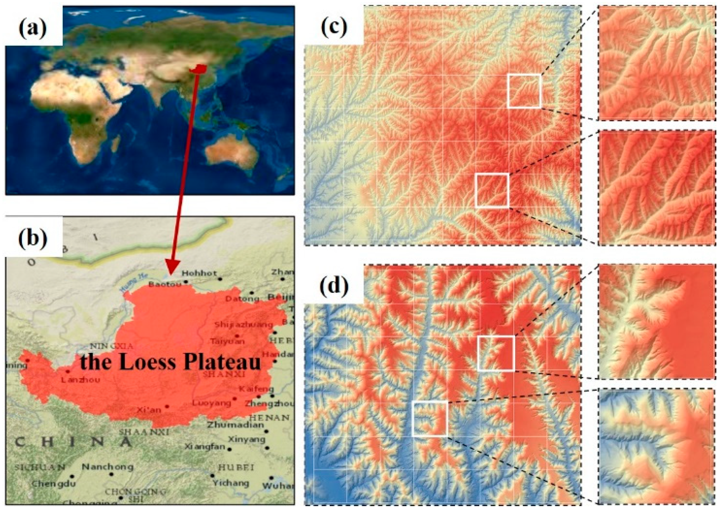
2.1. Study Object and Areas

We selected the loess landform as the study object. The loess landforms are formed by the deposition of silt with a small amount of silty-sand, which are easily eroded by water, wind, and glacial activity [41]. In this study, we focused on the topographic characteristics on landform surface, with the geological features of loess landform not considered. We collected terrain data from the Loess Plateau, China. The Loess Plateau contains typical loess landforms and covers an area of 640,000 km². For loess landforms, especially for those in the Loess Plateau, due to the stable geological basis, water erosion with different densities becomes the most important factor that influences the shape of the surface in this area. Under such a circumstance, the terrain in the Loess Plateau can be abstracted into a series of simple features. These terrain features are regarded as the basic representation of the loess landform and can support terrain generation. Meanwhile, these features can be regarded as the input data of GAN and provide topographic information to a DL-based model.

2.2. Data Preparation

2.2.1. DEM Data

A large amount of sample data is generally needed for DL algorithms. DEMs with a resolution of 5 m provided by the National Administration of Surveying (China) were used in this study. The complete areas were clipped to small patches of the same size (Figure 1). Patch size is an important parameter in this step. The memory occupation will increase rapidly and affect the system performance and training speed when the size is too large. If the size is too small, the information carried by patches cannot meet the requirement of the training process, and models may achieve unsatisfactory performances [42]. A patch size of 256 × 256 pixels was selected in this study, and the area of each sample was approximately 1.64 km² (1.28 km × 1.28 km). The topographic features of loess landforms can be clearly observed on these patches (Figure 1), and the computation and timing consumption are also accepted at this scale.

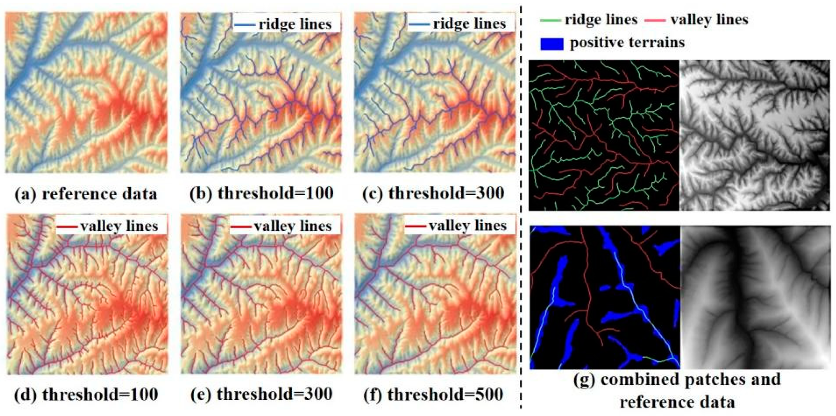
2.2.2. Input Terrain Features

We extracted different topographic features from sample DEMs as input conditions of the training process. For the loess landform, which is significantly influenced by water erosion, clear ridges and gullies can be observed in the study area, especially in the region of loess ridges and loess hills [3,43]. These lines compose the basic structure of the loess landform [44]. Another reason why we choose ridge and gully lines as input conditions is that lines with different lengths and densities can be extracted by setting various thresholds in the hydrological algorithm. During this process, the use of different flow accumulation thresholds can generate networks of ridge and gully lines with different densities [45]. With a small threshold, the resulting networks are dense and reveal the detailed relief of terrains, whereas using a large threshold provides a spare network and only shows the skeleton of the confluence relationship. Experiments based on different datasets can investigate the effect of line features with different quantitative characteristics on terrain generation. The reference DEM and extraction results of ridge and valley lines can be found in Figure 2a–f.

In addition, the loess landform can be basically separated into positive and negative terrains [46,47]. Negative terrains generally have high relief and are formed by intensive erosion in loess landforms, such as gully erosion. The topographic characteristics of negative terrain can be generally described by gully lines. However, the information provided by ridge lines is not enough to express the topographic characteristics of the positive terrain. The area of positive terrain is usually flat and has a moderate slope. Feature lines cannot achieve satisfactory performance in generating relatively flat surfaces with large areas. Therefore, despite the line features, we also extract the area of positive terrain and use it as one input feature in the training process. The introduction of areas of positive terrain helps understand the efficiency of surface elements in DL-based algorithms of terrain generation. Here, we use the method outlined in Xiong et al. (2014b) to extract positive terrains. The identification method includes calculating the mean value of DEM through neighborhood statistical analysis, calculating the difference between the original DEM and the mean of DEM, and finally implementing a binary classification to generate positive and negative terrain. Areas marked by blue in Figure 2g show the positive terrain areas.

The amount of training data directly affects the performance of CGANs. A large number of samples can effectively improve the model performance and reduce the effect of overfitting [48,49]. We constructed 4000 sample patches from the original DEMs to train the model. Each sample patch contains two parts, one 3-band image, and one DEM. We extracted the topographic features and organized them as a 3-band image. Gully lines, ridge lines, and positive areas are stored in bands 1, 2, and 3 in the image, respectively (Figure 2g). DEM data are also clipped to the same size as the corresponding image.

2.3. DL-Based Algorithm for Terrain Generation

In our study, a special CGAN, called Terrain-CGAN, is constructed to generate simulated terrain. The traditional CGAN, Pix2Pix, and algorithms in the field of computing methodologies were used as the basic framework of Terrain-CGAN, and some modifications were also taken to promote the performance of the generating process.

2.3.1. Basic Principle of CGAN

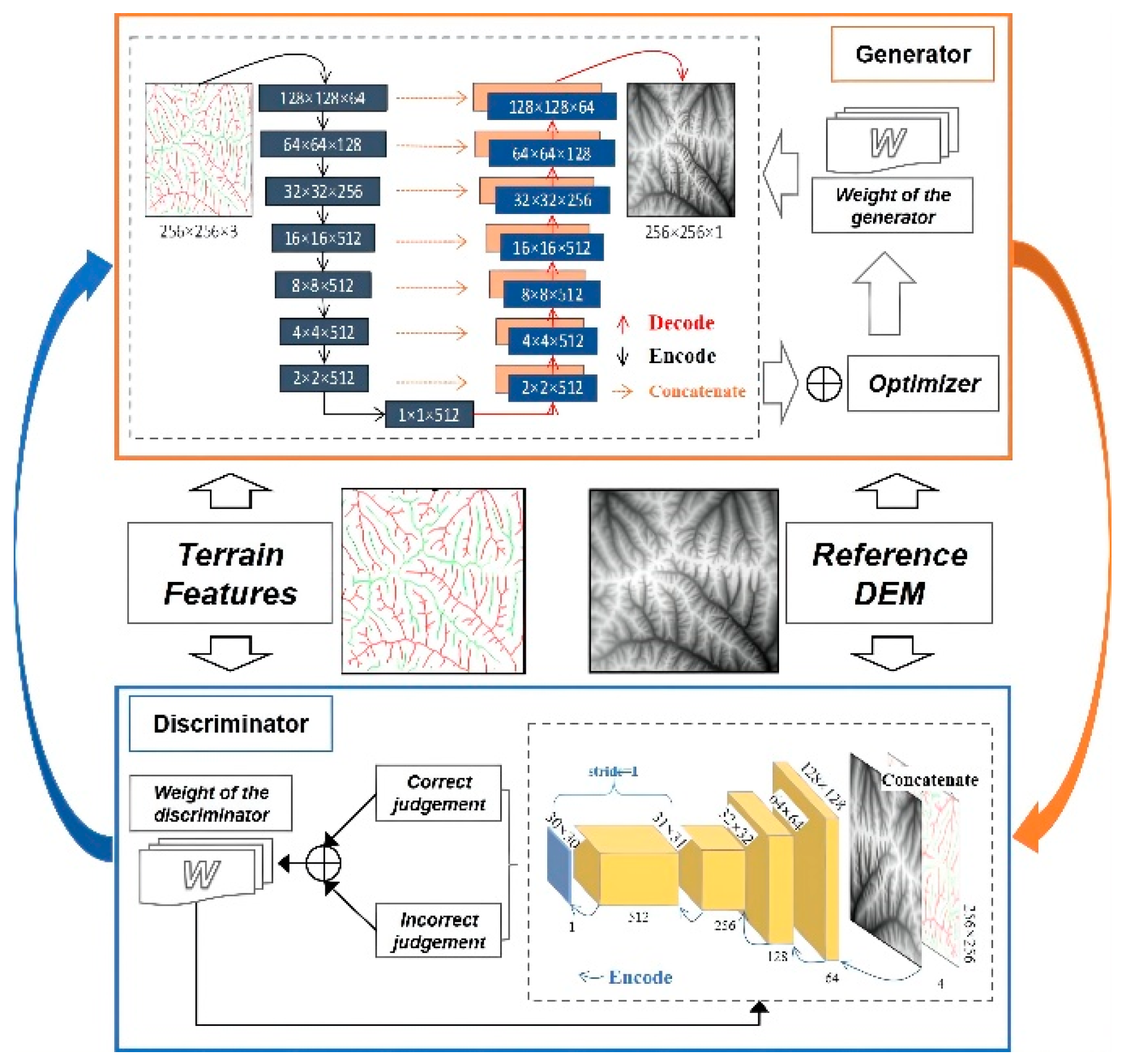
CGANs were developed based on GANs and have become some of the most powerful network structures in the field of terrain generation [27,28]. CGANs can generate specific results according to predefined requirements and avoid random plausible outputs, unlike traditional GANs. The typical architecture of CGANs can be separated into two main parts: the generator and discriminator [36]. The generator uses the encoder-decoder to transform the input data, commonly including the input image and other conditions, to obtain the output result. The discriminator is made up of several convolutional layers. This part can measure the similarity of the input data to the reference data and judge if the input data are generated by the generator or if the input data are the simulated sample. The overall loss that influences the CGAN is usually designed as:

$$L_{CGAN}=e{L}_1+L_G+L_D$$

(1)

where $e$ is an empirical scaling parameter, and, $L_1$, $L_G$, and $L_D$ are three basic loss functions [36]. The generator is influenced by $L_1$ and $L_G$, while $L_D$ influences the discriminator. This model follows a two-player min-max adversarial game, and eventually, the optimal CGAN are obtained as follows:

$$Optimal\left(G,D\right)=\underset{G}{min} \underset{D}{min} L_{CGAN}$$

(2)

Through this competition, the generator G and discriminator D obtain the capability to generate realistic data and distinguish generated data from the ground truth data, respectively [18].

Although the CGAN achieves the supervised framework based on GANs, the typical structure of the generator part has difficulty generating sufficient connections between the input conditions and generated results, which may lead to redundant and repetitive outputs and cause the model to collapse.

2.3.2. Terrain-CGAN

Further development of CGANs has been presented to promote the control efficiency of the input condition. The Pix2Pix architecture [35] is developed based on CGAN to learn a function to ‘translate’ the map from an input image to an output image. The most significant improvement of Pix2Pix net is the changing of the introduction of concatenation, which helps to retain original feature of input image and utilize the user-defined conditions [35]. The improved architecture has been proven to achieve more satisfactory results compared with typical CGANs in the field of background masking, image translation [35,50,51], etc. Therefore, to achieve the detection of correct topographic features from the input condition and generate the output that conforms to the specific landform, Terrain-CGAN is inspired by the above architectures and previous studies focusing on terrain generation [27,28]. In Terrain-CGAN (Figure 3), the basic structure of the Pix2Pix network is retained to achieve the efficient learning of topographic characteristics. The input data of Terrain-CGAN correspond to the sample unit we constructed in Section 2.2.2. The terrain features, including ridge lines, gully lines, and areas of positive terrain, are regarded as the input data to guide the learning process. The corresponding DEM in each sample pair is used as the target of the generating process, which means that the model is encouraged to construct a simulated DEM and make it similar to the referenced DEM. At the end of the training process, the trained model can extract topographic information from the input features and build a DEM that can express the terrain it learned. We set the learning rate to 0.0002 and selected Adam as the optimizer in Terrain-CGAN. The final model is completed after 500 epochs, which consumes approximately 8 h.

2.4. Experiments

Here, the experiments are mainly divided into two goals. (1) To investigate the effects of different topographic features on terrain generation, different data combinations are constructed and used as the input data to train models.

Table 1. Combinations of different terrain features.

	Component	Terrain Features
Case 1	Single terrain feature	Gully lines
Case 2		Ridge lines
Case 3	Multiple terrain features	Gully and ridge lines
Case 4		Gully lines, ridge lines, and positive terrain areas

shows the information about these data combinations. We first used a single topographic feature to train our model and then combined them for model training. (2) Ridge and gully lines with different amounts are generated and combined to discuss the influence of feature lines. As mentioned in Section 2.2.2, the length and number of ridge and gully lines can be controlled by setting different thresholds. We employed 100, 300, 500, 1000, 1500, and 2000, which are commonly used in digital terrain analysis to extract stream networks, as thresholds and extracted feature lines based on these thresholds. Values that are greater than 2000 were not applied in these experiments because extracted feature lines remain stable and exhibit only a little difference when the threshold is greater than 2000. All topographic lines were combined with the features of positive terrain and then used as input data for the models. Information about these experiments can be found in

Table 2. Combinations of features with different extraction thresholds.

	Threshold (for the Extraction of Line Features)	Terrain Features
Case A	100	Gully lines, ridge lines, and positive terrain areas
Case B	300
Case C	500
Case D	1000
Case E	1500
Case F	2000

.

2.5. Performance Evaluation

The performance assessment is explored from three perspectives: (1) Visual inspection is exploited to check if the generated results retain the basic characteristics of the loess landform, and the distribution of landform units can also be obtained through visual investigation. (2) Elevation analysis is performed to evaluate the relation between the generated results and the reference data by drawing a scatter graph and calculating the Pearson correlation coefficient. In this step, the elevation is normalized into the range of 0 through 1. (3) The surface slope is selected as the representative terrain derivative to assess the model performance. Slope is a basic terrain derivative and can efficiently reflect surface morphological features. The slope histogram is conducted to compare the difference between the reference data and the simulated results. In addition, the difference in surface slope between the generated results and the reference data is calculated in this step to assess whether the generated results achieve similar terrain to the original data.

3. Results

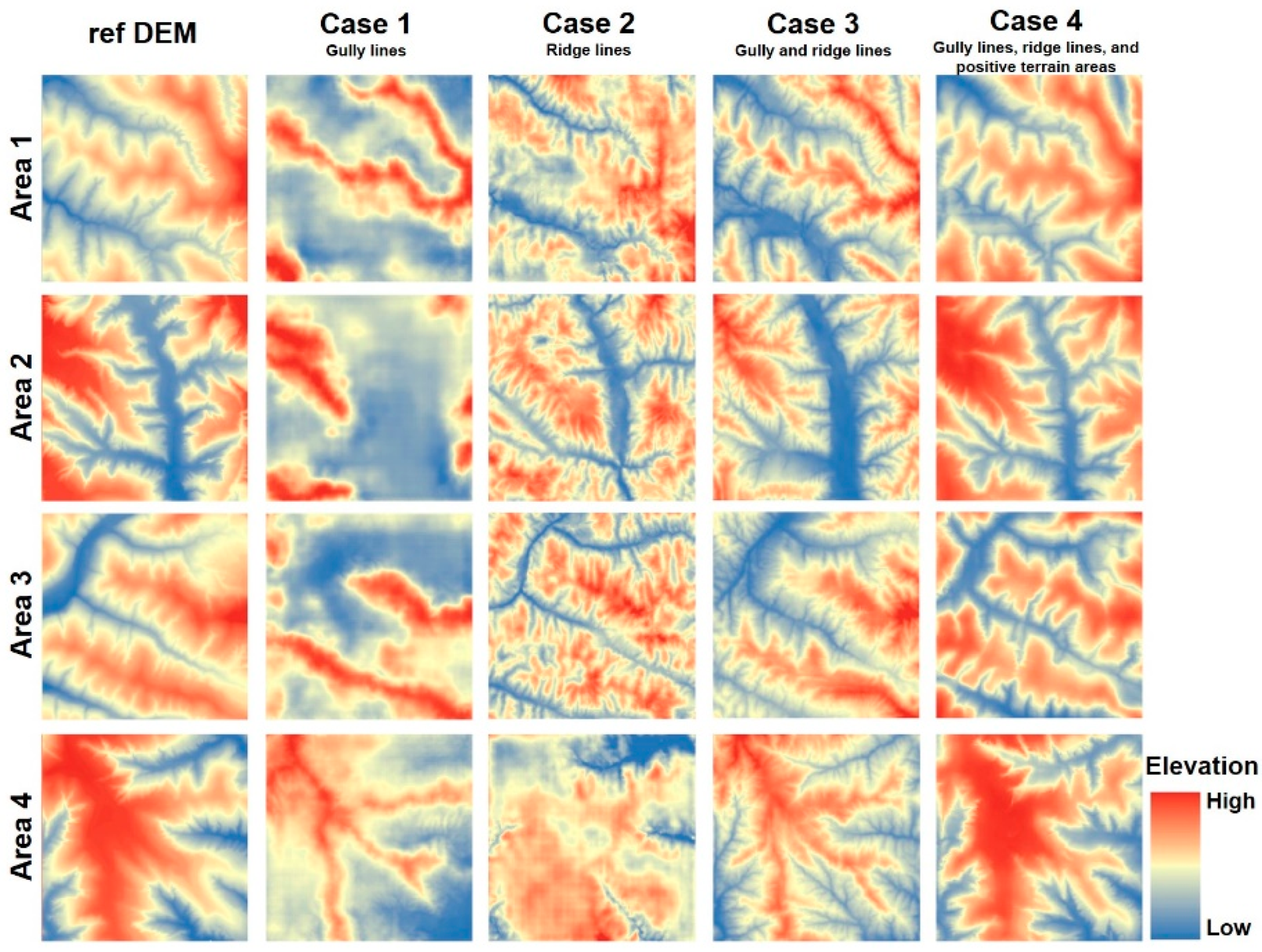
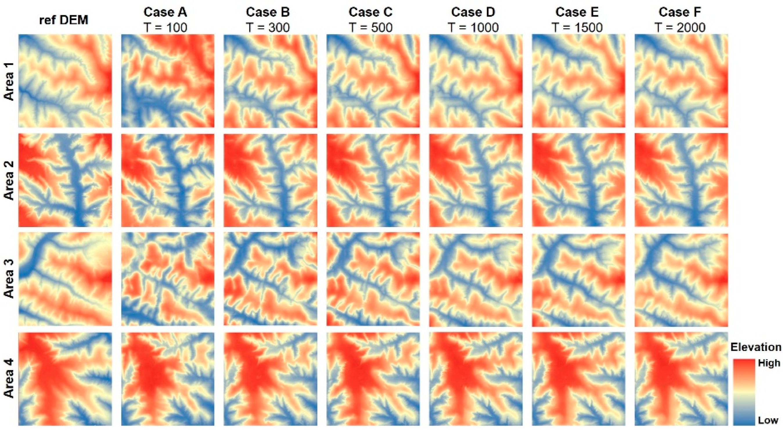
3.1. Results Based on Different Topographic Features

Four Terrain-CGANs were trained using different combinations of topographic features, and we compared their performance in four areas. Figure 4 shows that the results based on the single topographic feature have poor performances in terrain modelling. The model based on the ridge line cannot correctly build the ridge area, while the results based on the gully line also generate unsatisfactory terrain relief, even though the model correctly rebuilds several gullies in the correct spatial location. In addition, the combined topographic features improved the performance of terrain construction. The figures of Case 3 reflect more complete and continuous gullies and ridges than the results based on the single topographic features. Meanwhile, the model with positive terrain significantly outperformed the other models and constructed correct areas of the positive terrains, which cannot be observed in the other results. Therefore, it can be concluded that the model with the combined features of ridge lines, valley lines, and regions of positive terrain outperformed the other three models tested. The following comparison and analyses are all based on the combination of these three features.

We subsequently discuss the influence of topographic features with different densities. Commonly, high threshold values represent a low density of line features, and low thresholds mean that there are a range of ridge and gully lines existing in the input samples. Figure 5 shows that the model with a high density of line features generates more details than the models trained based on low densities. For example, some very small gullies can be easily observed in the boundary of the gully areas when the model employs high-density inputs. However, these details are not always positive features, which means that a part of the detailed terrain is generated through the inference of Terrain-CGAN and cannot be observed in the reference data. As shown in the results of Area 3, broken ridges can be observed in the result of Cases A, B, and C that are trained on the basis of line features with high density. In general, the results of Cases D, E, and F are better than those of Cases A, B, and C, and the generated terrain starts to be stable from Case D.

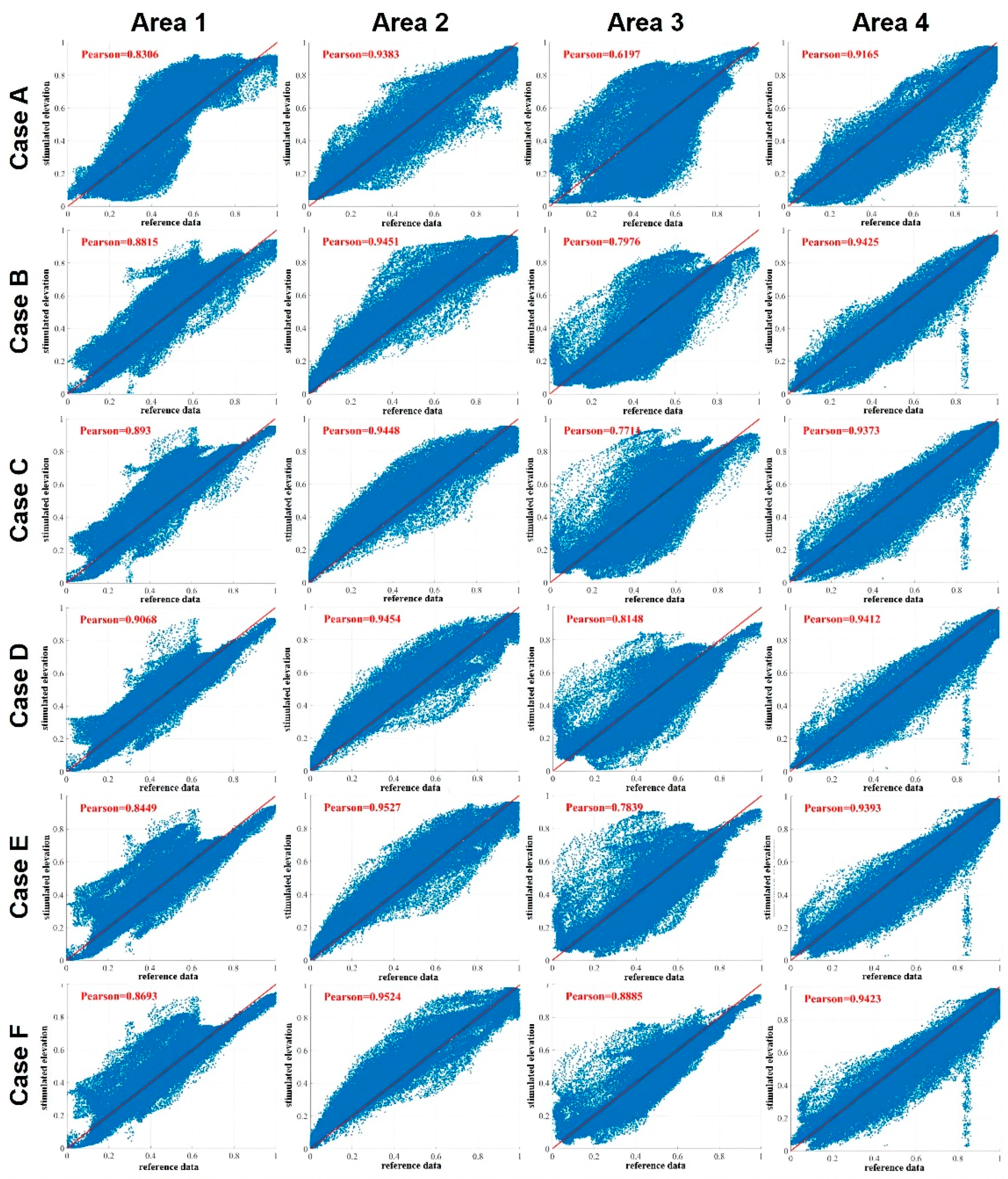
3.2. Elevation Analysis

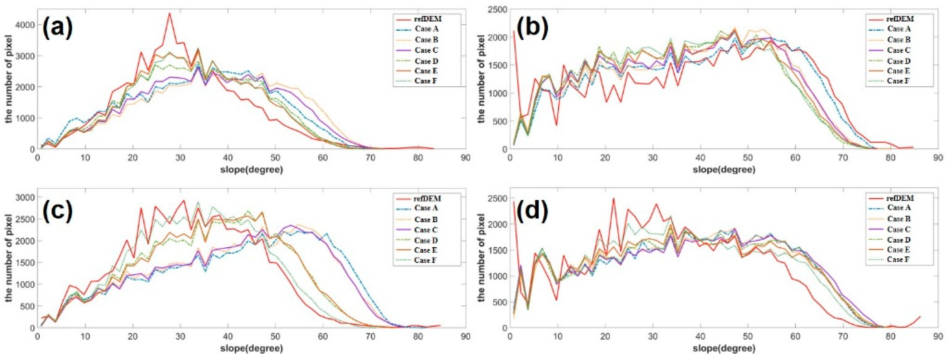
In this section, we map the elevation relation between the reference data and the generated results and calculate the Pearson correlation coefficient (Figure 6). The high coefficient indicates that the simulated results include topographic characteristics similar to those of the reference data. The coefficients in Areas 1, 3, and 4 are all greater than 0.8, which reflects the strong positive correlation between the generated results and the reference data. In addition, the Pearson coefficient tends to increase with increasing threshold. Cases D, E, and F generally achieve higher coefficients than Cases A, B, and C, which is consistent with what we observed in Section 3.1. However, Area 3, which includes broken ridges in Figure 5, contains unsatisfactorily low correlation coefficients. Complex terrain relief could be the primary reason for the unexpected deviation from the reference data.

3.3. Slope Analysis

Figure 7 shows the slope of different results. Generally, most results achieved a trend similar to that of the reference data. In Areas 2 and 4, the results of Terrain-CGAN exhibit similar fluctuations to the reference data in the range of 30° to 50°. Meanwhile,

Table 3. The statistics of surface slope. Ref DEM represents the reference data.

		Mean	Median	Standard Deviation	Maximum
Area 1	Ref DEM	30.91	29.69	12.46	82.55
	Case A	34.29	35.26	14.29	70.76
	Case B	37.61	38.13	14.56	72.45
	Case C	36.10	36.34	14.20	73.49
	Case D	33.11	32.99	13.03	71.68
	Case E	32.68	32.31	12.39	72.38
	Case F	33.09	32.63	12.47	73.02
Area 2	Ref DEM	38.90	41.47	20.12	85.15
	Case A	39.28	40.73	18.08	77.88
	Case B	37.28	38.93	17.44	79.70
	Case C	36.83	38.13	17.34	77.07
	Case D	35.59	36.59	16.67	75.58
	Case E	36.05	36.87	17.08	77.92
	Case F	35.41	36.09	16.72	76.09
Area 3	Ref DEM	32.34	32.31	13.64	84.71
	Case A	42.22	44.49	17.29	81.61
	Case B	41.35	43.21	16.75	77.87
	Case C	41.43	43.59	16.61	77.86
	Case D	36.41	37.41	14.38	75.08
	Case E	36.68	37.79	14.22	75.88
	Case F	33.63	34.04	13.21	70.76
Area 4	Ref DEM	32.99	32.51	17.59	86.90
	Case A	37.46	38.58	18.59	78.66
	Case B	37.50	38.66	18.49	79.79
	Case C	38.02	39.14	19.00	79.43
	Case D	37.48	38.13	18.60	78.80
	Case E	36.79	36.93	18.48	79.36
	Case F	35.45	35.06	17.95	78.95

shows that the Terrain-CGAN can generate a small deviation in the mean slope. In addition, the lowest difference in the mean slope between the generated results and the reference data usually occurs in Case F with the highest threshold. Even though the terrain generated by Terrain-CGAN is close to the reference surface, especially in Areas 2 and 4, several unexpected deviations still exist. For example, in Area 1, Terrain-CGAN fails to construct the peak on the slope curvature (Figure 7a). We think this error around peaks is acceptable given that the overall trend constructed by Terrain-CGAN matches the reference data in most ranges.

4. Discussion

4.1. Influence of Different Terrain Cues and Feature Combinations

A range of previous research has proven that terrain cues can significantly improve a model’s performance in generating terrain. However, the question as to which types of terrain cues should be used and how to combine them to generate reliable terrain still needs further discussion. Through our experiments, we suggest that the main landform units that form targeted terrain should be determined before the launch of the algorithm, and the characteristics of these units should be regarded as the key features in selecting terrain cues that are used as the model’s input. In this study, we consider the basic structure of the loess landform consisting of ridge and gully lines and introduce the positive terrain as one of the input data to optimize the construction process. The results show that the input combination including positive terrain significantly helps construct valid terrain, especially in flat areas with small surface slopes (Figure 8). The topographic frame is also optimized through the introduction of positive terrain. Therefore, the selection of terrain cues should consider the differences in landforms and surface morphology. Key terrain cues should be found and used as the input of the CGAN model to generate high-quality data with low competition and data costs. In addition, previous research has mainly discussed the usability of line and point features. In our study, we introduce one surface feature, positive terrain area, to improve the quality of the generated results. As shown in Figure 4, the available surface features can be integrated into input data and improve the model’s ability to restore accurate terrain.

However, there are still issues that need further discussion. For example, due to the uncertainty in GAN, the positive terrain areas generated by our method are not as flat as reference data, and these detailed reliefs could influence the subsequent morphological or hydrological analysis based on DEMs. In addition, the number of line features should also be carefully considered in terrain generation. The results show that the best expression of detailed terrain and the best slope results cannot be simultaneously found in one model, which suggests that the great expression of the detailed terrain could lead to an unexpected slope histogram. In some cases, detailed terrains could be considered noise and would disturb the terrain analyses. Therefore, before the launch of terrain generation algorithm, we should construct a bridge between the purposes of applications or studies and the determination of terrain features for model training. In other words, we should determine which information is the most important part for research and then choose a suitable model and training dataset to generate reliable terrain data. Finally, relative studies focusing on other landforms can also benefit from our method, but it is critical to determine the input topographic features. In the Loess Plateau, water erosion is the most important factor that influences landform evolution and is much more significant than other factors, which makes it valid to abstract terrain based on simple lines and areas. However, for other landforms with more than one dominant geomorphological factor, we suggest that the present framework is available but the input features must be adjusted according to the dominant factors.

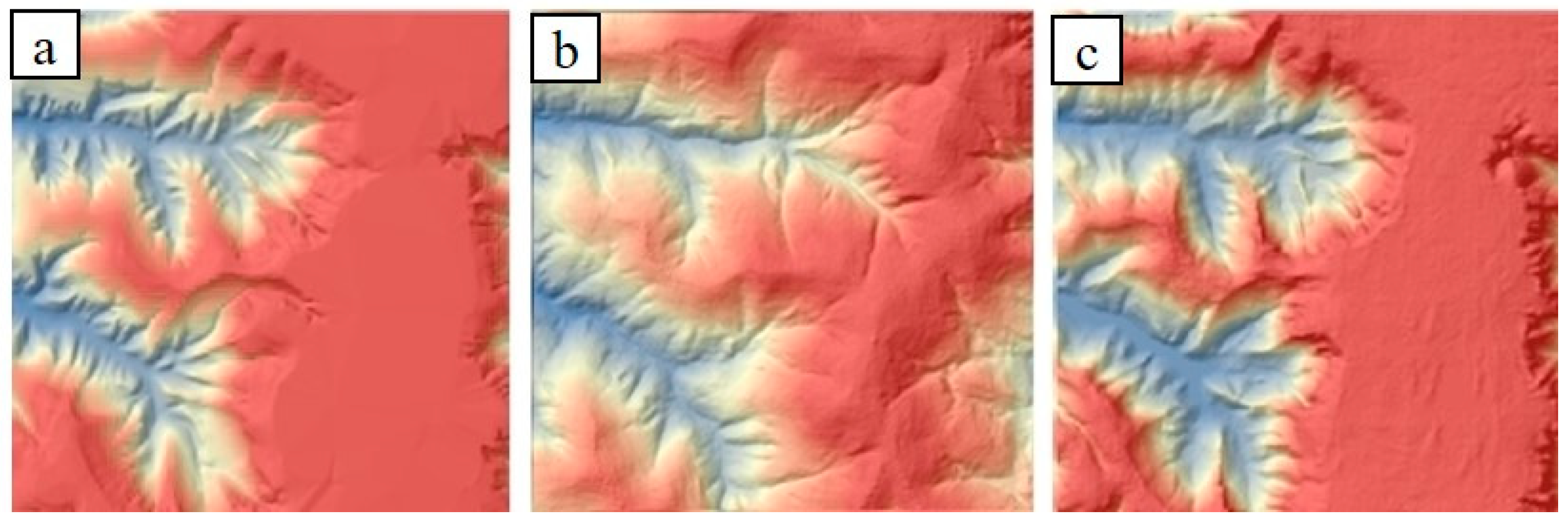
4.2. Applications of Terrain-CGAN

The output of the Terrain-CGAN can be the representation of the true surface and the ‘virtual’ simulated terrain [27]. The second type of data contain similar characteristics to one specific landform, but they do not belong to any place on Earth. Simulated topographic data can be widely applied in constructing virtual scenes, simulating landform evolution, and supporting the development of intelligent geographical algorithms. As shown in Figure 9, ridge and gully lines, which represent different development stages of loess landforms, are used as the input of our model to construct terrain data, and the generated results successfully reconstruct the process of vertical and lateral erosion. Landform development can be remerged based on low data and computing consumption. In addition, previous studies have proven that terrain data benefit landform classification, object detection, and geography-related research [16,52,53,54,55]. The fine-tuned model can quickly generate topographic data with simple input data and support related studies, especially DL-based algorithms that require a large amount of input data.

5. Conclusions

A DL-based algorithm called Terrain-CGAN inspired by a previous study was constructed to generate topographic data of the loess landforms based on topographic feature lines and areas, including ridge lines, gully lines, and areas of positive terrain. The positive terrain area, which is a special unit existing in loess landform areas, significantly improved the accuracy of simulated results. The fine-trained model can quickly generate a large amount of data that contain similar elevation and slope characteristics with loess landform.

The topographic data generated by our method has the potential to be used in geographic studies that need topographic data. Experiments based on simulation data are common in geographic research. The simulation data conforming to the characteristics of specific landforms can support studies such as simulating landform evolution. In addition, the proposed framework could be transferred to other landform areas.

References

1. Drăguţ, L.; Dornik, A. Land-surface segmentation as a method to create strata for spatial sampling and its potential for digital soil mapping. Int. J. Geogr. Inf. Sci. 2016, 30, 1359–1376. [Google Scholar] [CrossRef] [Green Version]
2. Evans, I.S. Geomorphometry and landform mapping: What is a landform? Geomorphology 2012, 137, 94–106. [Google Scholar] [CrossRef]
3. Li, S.; Xiong, L.; Tang, G.; Strobl, J. Deep learning-based approach for landform classification from integrated data sources of digital elevation model and imagery. Geomorphology 2020, 354, 107045. [Google Scholar] [CrossRef]
4. Liu, K.; Song, C.; Ke, L.; Jiang, L.; Ma, R. Automatic watershed delineation in the Tibetan endorheic basin: A lake-oriented approach based on digital elevation models. Geomorphology 2020, 358, 107127. [Google Scholar] [CrossRef]
5. Sesnie, S.E.; Gessler, P.E.; Finegan, B.; Thessler, S. Integrating Landsat TM and SRTM-DEM derived variables with decision trees for habitat classification and change detection in complex neotropical environments. Remote Sens. Environ. 2008, 112, 2145–2159. [Google Scholar] [CrossRef]
6. Hu, G.; Wang, C.; Li, S.; Dai, W.; Xiong, L.; Tang, G.; Strobl, J. Using vertices of a triangular irregular network to calculate slope and aspect. Int. J. Geogr. Inf. Sci. 2021, 226, 103944. [Google Scholar] [CrossRef]
7. Drăguţ, L.; Blaschke, T. Automated classification of landform elements using object-based image analysis. Geomorphology 2006, 81, 330–344. [Google Scholar] [CrossRef]
8. Hu, G.; Dai, W.; Li, S.; Xiong, L.; Tang, G.; Strobl, J. Quantification of terrain plan concavity and convexity using aspect vectors from digital elevation models. Geomorphology 2021, 375, 107553. [Google Scholar] [CrossRef]
9. Székely, B.; Karátson, D. DEM-based morphometry as a tool for reconstructing primary volcanic landforms: Examples from the Börzsöny Mountains, Hungary. Geomorphology 2004, 63, 25–37. [Google Scholar] [CrossRef]
10. Székely, B.; Zámolyi, A.; Draganits, E.; Briese, C. Geomorphic expression of neotectonic activity in a low relief area in an Airborne Laser Scanning DTM: A case study of the Little Hungarian Plain (Pannonian Basin). Tectonophysics 2009, 474, 353–366. [Google Scholar] [CrossRef]
11. Xiong, L.; Tang, G.; Yang, X.; Li, F. Geomorphology-oriented digital terrain analysis: Progress and perspectives. J. Geogr. Sci. 2021, 31, 456–476. [Google Scholar] [CrossRef]
12. Yang, X.; Na, J.; Tang, G.; Wang, T.; Zhu, A. Bank gully extraction from DEMs utilizing the geomorphologic features of a loess hilly area in China. Front. Earth Sci. 2019, 13, 151–168. [Google Scholar] [CrossRef]
13. Zhao, W.; Duan, S.-B.; Li, A.; Yin, G. A practical method for reducing terrain effect on land surface temperature using random forest regression. Remote Sens. Environ. 2019, 221, 635–649. [Google Scholar] [CrossRef]
14. Lv, G.; Xiong, L.; Chen, M.; Tang, G.; Sheng, Y.; Liu, X.; Song, Z.; Lu, Y.; Yu, Z.; Zhang, K. Chinese progress in geomorphometry. J. Geogr. Sci. 2017, 27, 1389–1412. [Google Scholar] [CrossRef]
15. Li, W.; Hsu, C.-Y. Automated terrain feature identification from remote sensing imagery: A deep learning approach. Int. J. Geogr. Inf. Sci. 2020, 34, 637–660. [Google Scholar] [CrossRef]
16. Hsu, C.-Y.; Li, W.; Wang, S. Knowledge-Driven GeoAI: Integrating Spatial Knowledge into Multi-Scale Deep Learning for Mars Crater Detection. Remote Sens. 2021, 13, 2116. [Google Scholar] [CrossRef]
17. Janowicz, K.; Gao, S.; McKenzie, G.; Hu, Y.; Bhaduri, B. GeoAI: Spatially explicit artificial intelligence techniques for geographic knowledge discovery and beyond. Int. J. Geogr. Inf. Sci. 2020, 34, 625–636. [Google Scholar] [CrossRef]
18. Li, S.; Hu, G.; Cheng, X.; Xiong, L.; Tang, G.; Strobl, J. Integrating topographic knowledge into deep learning for the void-filling of digital elevation models. Remote Sens. Environ. 2022, 269, 112818. [Google Scholar] [CrossRef]
19. Wilson, J.P. Digital terrain modeling. Geomorphology 2012, 137, 107–121. [Google Scholar] [CrossRef]
20. Galin, E.; Guérin, E.; Peytavie, A.; Cordonnier, G.; Cani, M.P.; Benes, B.; Gain, J. A review of digital terrain modeling. Comput. Graph. Forum 2019, 38, 553–577. [Google Scholar] [CrossRef]
21. Zhou, Q.; Zhu, A.X. The recent advancement in digital terrain analysis and modeling. Int. J. Geogr. Inf. Sci. 2013, 27, 1269–1271. [Google Scholar] [CrossRef]
22. Génevaux, J.-D.; Galin, É.; Guérin, E.; Peytavie, A.; Benes, B. Terrain generation using procedural models based on hydrology. ACM Trans. Graph. (TOG) 2013, 32, 1–13. [Google Scholar] [CrossRef] [Green Version]
23. Raffe, W.L.; Zambetta, F.; Li, X. A survey of procedural terrain generation techniques using evolutionary algorithms. In Proceedings of the 2012 IEEE Congress on Evolutionary Computation, Brisbane, QLD, Australia, 10–15 June 2012; pp. 1–8. [Google Scholar]
24. Rose, T.J.; Bakaoukas, A.G. Algorithms and approaches for procedural terrain generation-a brief review of current techniques. In Proceedings of the 2016 8th International Conference on Games and Virtual Worlds for Serious Applications (VS-GAMES), Barcelona, Spain, 7–9 September 2016; pp. 1–2. [Google Scholar]
25. Smelik, R.M.; De Kraker, K.J.; Tutenel, T.; Bidarra, R.; Groenewegen, S.A. A survey of procedural methods for terrain modelling. In Proceedings of the CASA Workshop on 3D Advanced Media In Gaming And Simulation (3AMIGAS), Amsterdam, The Netherlands, 16 June 2009; pp. 25–34. [Google Scholar]
26. Cordonnier, G.; Galin, E.; Gain, J.; Benes, B.; Guérin, E.; Peytavie, A.; Cani, M.-P. Authoring landscapes by combining ecosystem and terrain erosion simulation. ACM Trans. Graph. (TOG) 2017, 36, 1–12. [Google Scholar] [CrossRef] [Green Version]
27. Guérin, É.; Digne, J.; Galin, E.; Peytavie, A.; Wolf, C.; Benes, B.; Martinez, B. Interactive example-based terrain authoring with conditional generative adversarial networks. Acm Trans. Graph. (TOG) 2017, 36, 1–13. [Google Scholar] [CrossRef] [Green Version]
28. Zhu, D.; Cheng, X.; Zhang, F.; Yao, X.; Gao, Y.; Liu, Y. Spatial interpolation using conditional generative adversarial neural networks. Int. J. Geogr. Inf. Sci. 2020, 34, 735–758. [Google Scholar] [CrossRef]
29. Krizhevsky, A.; Sutskever, I.; Hinton, G.E. ImageNet classification with deep convolutional neural networks. In Advances in Neural Information Processing Systems; Curran Associates, Inc.: New York, NY, USA, 2012; pp. 1097–1105. [Google Scholar]
30. Zhong, Y.; Zhu, Q.; Zhang, L. Scene classification based on the multifeature fusion probabilistic topic model for high spatial resolution remote sensing imagery. IEEE Trans. Geosci. Remote Sens. 2015, 53, 6207–6222. [Google Scholar] [CrossRef]
31. Li, K.; Wan, G.; Cheng, G.; Meng, L.; Han, J. Object detection in optical remote sensing images: A survey and a new benchmark. ISPRS J. Photogramm. Remote Sens. 2020, 159, 296–307. [Google Scholar] [CrossRef]
32. Gregor, K.; Danihelka, I.; Graves, A.; Rezende, D.J.; Wierstra, D. DRAW: A recurrent neural network for image generation. Comput. Sci. 2015, 37, 1462–1471. [Google Scholar]
33. Gatys, L.A.; Ecker, A.S.; Bethge, M. Texture Synthesis Using Convolutional Neural Networks. Adv. Neural Inf. Process. Syst. 2015, 70, 262–270. [Google Scholar]
34. Gatys, L.A.; Ecker, A.S.; Bethge, M. Image style transfer using convolutional neural networks. In Proceedings of the IEEE Conference on Computer Vision and Pattern Recognition, Las Vegas, NV, USA, 27–30 June 2016; pp. 2414–2423. [Google Scholar]
35. Isola, P.; Zhu, J.-Y.; Zhou, T.; Efros, A.A. Image-to-image translation with conditional adversarial networks. In Proceedings of the IEEE Conference on Computer Vision and Pattern Recognition, Honolulu, HI, USA, 21–26 July 2017; pp. 1125–1134. [Google Scholar]
36. Mirza, M.; Osindero, S. Conditional generative adversarial nets. arXiv 2014, arXiv:1411.1784. [Google Scholar]
37. Dachsbacher, C.; Meyer, M.; Stamminger, M. Height-Field Synthesis by Non-Parametric Sampling. In Vision, Modeling and Visualization 2005; University of Erlangen-Nuremberg: Erlangen, Germany, 2005; pp. 297–302. [Google Scholar]
38. Goodfellow, I.J.; Pouget-Abadie, J.; Mirza, M.; Xu, B.; Warde-Farley, D.; Ozair, S.; Courville, A.; Bengio, Y. Generative adversarial nets. In Proceedings of the International Conference on Neural Information Processing Systems, Montreal, QC, Canada, 8–13 December 2014; pp. 2672–2680. [Google Scholar]
39. Yuan, Q.; Shen, H.; Li, T.; Li, Z.; Li, S.; Jiang, Y.; Xu, H.; Tan, W.; Yang, Q.; Wang, J. Deep learning in environmental remote sensing: Achievements and challenges. Remote Sens. Environ. 2020, 241, 111716. [Google Scholar] [CrossRef]
40. Li, T.; Shen, H.; Yuan, Q.; Zhang, L. Geographically and temporally weighted neural networks for satellite-based mapping of ground-level PM2.5. ISPRS J. Photogramm. Remote Sens. 2020, 167, 178–188. [Google Scholar] [CrossRef]
41. Fu, B. Soil erosion and its control in the Loess Plateau of China. Soil Use Manag. 1989, 5, 76–82. [Google Scholar] [CrossRef]
42. Li, S.; Xiong, L.; Hu, G.; Dang, W.; Tang, G.; Strobl, J. Extracting check dam areas from high-resolution imagery based on the integration of object-based image analysis and deep learning. Land Degrad. Dev. 2021, 32, 2303–2317. [Google Scholar] [CrossRef]
43. Xiong, L.-Y.; Tang, G.-A.; Li, F.-Y.; Yuan, B.-Y.; Lu, Z.-C. Modeling the evolution of loess-covered landforms in the Loess Plateau of China using a DEM of underground bedrock surface. Geomorphology 2014, 209, 18–26. [Google Scholar] [CrossRef]
44. Xiong, L.; Tang, G.; Yuan, B.; Lu, Z.; Li, F.; Zhang, l. Geomorphological inheritance for loess landform evolution in a severe soil erosion region of Loess Plateau of China based on digital elevation models. Sci. China Earth Sci. 2014, 57, 1944–1952. [Google Scholar] [CrossRef]
45. Jenson, S.K.; Domingue, J.O. Extracting topographic structure from digital elevation data for geographic information system analysis. Photogramm. Eng. Remote Sens. 1988, 54, 1593–1600. [Google Scholar]
46. Zhou, Y.; Yang, X.; Xiao, C.; Zhang, Y.; Luo, M. Positive and negative terrains on northern Shaanxi Loess Plateau. J. Geogr. Sci. 2010, 20, 64–76. [Google Scholar] [CrossRef]
47. Xiong, L.; Tang, G.; Yan, S.; Zhu, S.; Sun, Y. Landform-oriented flow-routing algorithm for the dual-structure loess terrain based on digital elevation models. Hydrol. Process. 2014, 28, 1756–1766. [Google Scholar] [CrossRef]
48. Li, W.; Zhou, B.; Hsu, C.-Y.; Li, Y.; Ren, F. Recognizing terrain features on terrestrial surface using a deep learning model: An example with crater detection. In Proceedings of the 1st Workshop on Artificial Intelligence and Deep Learning for Geographic Knowledge Discovery, Los Angeles, CA, USA, 7–10 November 2017; pp. 33–36. [Google Scholar]
49. Zhang, W.; Witharana, C.; Liljedahl, A.K.; Kanevskiy, M. Deep convolutional neural networks for automated characterization of arctic ice-wedge polygons in very high spatial resolution aerial imagery. Remote Sens. 2018, 10, 1487. [Google Scholar] [CrossRef] [Green Version]
50. Dietrich-Sussner, R.; Davari, A.; Seehaus, T.; Braun, M.; Christlein, V.; Maier, A.; Riess, C. Synthetic Glacier SAR Image Generation from Arbitrary Masks Using Pix2Pix Algorithm. arXiv 2021, arXiv:2101.03252. [Google Scholar]
51. Armanious, K.; Jiang, C.; Fischer, M.; Küstner, T.; Hepp, T.; Nikolaou, K.; Gatidis, S.; Yang, B. MedGAN: Medical image translation using GANs. Comput. Med. Imaging Graph. 2020, 79, 101684. [Google Scholar] [CrossRef] [PubMed]
52. Qin, C.-Z.; Bao, L.-L.; Zhu, A.X.; Wang, R.-X.; Hu, X.-M. Uncertainty due to DEM error in landslide susceptibility mapping. Int. J. Geogr. Inf. Sci. 2013, 27, 1364–1380. [Google Scholar] [CrossRef]
53. Dai, W.; Na, J.; Huang, N.; Hu, G.; Yang, X.; Tang, G.; Xiong, L.; Li, F. Integrated edge detection and terrain analysis for agricultural terrace delineation from remote sensing images. Int. J. Geogr. Inf. Sci. 2020, 34, 484–503. [Google Scholar] [CrossRef]
54. Gerçek, D.; Toprak, V.; Strobl, J. Object-based classification of landforms based on their local geometry and geomorphometric context. Int. J. Geogr. Inf. Sci. 2011, 25, 1011–1023. [Google Scholar] [CrossRef]
55. Penfound, E.; Vaz, E. Analysis of Wetland Landcover Change in Great Lakes Urban Areas Using Self-Organizing Maps. Remote Sens. 2021, 13, 4960. [Google Scholar] [CrossRef]
Figure 1. Example of sample data. (a,b) the location of the Loess Plateau; (c,d) the terrain in the Loess Plateau (the size of a small patch is 256 × 256 pixels).
Remotesensing 14 01166 g001
Figure 2. Representation of input patches. (a) Reference DEM; (b,c) The extraction of ridge lines based on different thresholds; (df) the extraction of valley lines on different thresholds; (g) the patches combining ridge lines, valley lines, positive terrains, and the corresponding DEM.
Remotesensing 14 01166 g002
Figure 3. The structure of Terrain-CGAN.
Remotesensing 14 01166 g003
Figure 4. Results based on the different combinations of topographic features. Ref DEM represents the reference data.
Remotesensing 14 01166 g004
Figure 5. Results based on the combinations generated by different thresholds. Ref DEM represents the reference data, and T represents the threshold for extracting stream network.
Remotesensing 14 01166 g005
Figure 6. Results based on the different combinations of topographic features. Ref DEM represents the reference data.
Remotesensing 14 01166 g006
Figure 7. Results based on the different combinations of topographic features. Ref DEM represents the reference data. (ad) represent results in four test areas, respectively.
Remotesensing 14 01166 g007
Figure 8. The influence of different terrain features. (a) Reference DEM; (b) trained by gully and ridge lines; (c) trained by gully lines, ridge lines and positive terrain.
Remotesensing 14 01166 g008
Figure 9. Simulating landform evolution based on different inputting terrain features. (ai) represent terrain features (left) and landforms of different periods (right), respectively.
Remotesensing 14 01166 g009