Varying Amplitude Vibration Phase Suppression Algorithm in ISAL Imaging

Abstract

Platform vibration introduces sinusoidal modulation in inverse synthetic aperture lidar (ISAL) imaging, which causes paired echoes in ISAL imaging. In this paper, a varying amplitude vibration phase suppression algorithm is proposed. Working without prior knowledge, the proposed algorithm can suppress paired echoes under the condition of varying vibration amplitude and will not introduce new phase errors. Furthermore, the method is suitable for the imaging scene without isolated points. Both the simulated and real experiment results of ISAL turntable data demonstrate the effectiveness of the proposed algorithm.

1. Introduction

Inverse synthetic aperture lidar (ISAL) has the same imaging principle as ISAR. It achieves high range resolution by transmitting large bandwidth signals and achieves high azimuth resolution using synthetic aperture technology. The wavelength of ISAL is in the order of microns, which is about 3–4 orders shorter than the wavelength of ISAR (inverse synthetic aperture radar). Therefore, ISAL can obtain a higher azimuth resolution within the same accumulated time, which can be applied to long-range two-dimensional imaging [1,2,3].

In ISAL, a single-channel transceiver system is commonly used to transmit the linear frequency modulation (LFM) signal for target imaging, identification and classification [4,5,6,7]. Since the wavelength of lidar is in the order of microns, ISAL is very sensitive to even a small platform vibration, which will introduce sinusoidal phase modulation into the returned signals. After Fourier transformation of the returned signals along the azimuth direction, paired echoes will be generated, which makes ‘ghost targets’ appear in the image [8,9,10,11]. The ‘ghost targets’ are false targets in images, which affect the performance of target identification and classification. Therefore, it is necessary to suppress paired echoes.

The suppression of paired echoes is realized by vibration phase compensation. Traditional vibration phase compensation for ISAR includes three steps. First, estimate vibration parameters, including vibration amplitude, frequency and the initial phase. Second, construct the sinusoidal modulation function of vibration phase according to the vibration parameters. Finally, compensate the vibration phase. At present, ISAR vibration parameter estimation methods based on a discrete fractional Fourier transform [12,13] and two-dimensional searching [14,15] can be used to obtain vibration phase if the phase is constant. However, since ISAL’s high sensitivity to platform vibration will make the vibration phase variable in real applications, these methods cannot be directly used to estimate the vibration phase of ISAL.

On the other hand, there are also some studies on the vibration phase compensation of ISAL, but the application of them is limited by special conditions. One study [16] proposed a vibration phase compensation method based on multichannel interference in which the vibration phase is estimated by high-order polynomial fitting, but this method works only for multichannel systems and not for single-channel systems. Another study [17] proposed a vibration phase compensation method based on the instantaneous ranging model for triangular frequency-modulated continuous wave (FMCW) signals. This method compensates the vibration phase by calculating the instantaneous ranges of up and down dechirp signals, but it is not suitable for LFM signals.

For these reasons, a vibration phase compensation method based on the delay conjugate multiplication of echoes is proposed in this paper which can suppress paired echoes under the condition of varying amplitude vibrations for a single-channel transceiver system transmitting the LFM signal. Firstly, range compression is performed on the echoes. Secondly, the signal from the same range cell is multiplied by the conjugate of its time delay, and the phase of the multiplication result is taken. Thirdly, the vibration phase is estimated by offsetting the amplitude modulation and time delay terms on this taken phase. Finally, the estimated vibration phase is compensated, and the paired echoes are suppressed. This method works without prior knowledge and will not introduce new phase errors. Furthermore, this method is suitable for the imaging scene without isolated points.

This paper is organized as follows. In Section 2, we introduce the ISAL turntable imaging model. The derivation procedure of the vibration phase estimation and the compensation algorithm are presented in Section 3. The simulated and real experiment results of ISAL turntable data are provided in Section 4. Finally, the conclusion is given in Section 5.

2. ISAL Turntable Imaging Model

2.1. Imaging Geometry

In ISAL, the synthetic aperture is obtained by the motion of the target. The motion of the target can generally be decomposed into translational motion and rotational motion. After the translational motion is compensated for, the imaging geometry can be equivalent to an ISAL turntable model in which the target rotates around a reference point. Figure 1 shows the ISAL turntable imaging geometry.

In Figure 1, the lidar is located at $L$, $o$ is the center of the turntable and the turntable rotates around $o$. The distance from $L$ to $o$ is $R_o$. The y-axis is in the direction of $\overrightarrow{LO}$, and the x-axis is perpendicular to the y-axis. Initially, the scattering point $S_{cat}$ is located at $P$. The distance from $P$ to $o$ is $r$, and $r\ll R_o$. The initial angle between $P$ and the x-axis is ${\theta }_0$. Assuming that the scattering point $S_{cat}$ rotates from $P$ to $P^{\prime }$ with angular velocity $\omega$, the rotation angle of $S_{cat}$ is $\Delta \theta =\omega t_m$, where $t_m$ is the slow time. When the platform is not vibrating, the distance $R$ from the radar to the scattering point $S_{cat}$ is as follows:

$$\begin{array}{l}R=\sqrt{R_0^2+r^2-2R_{0}r\cos \left({\theta }_o+\pi /2+\omega t_m\right)}\\ \begin{array}{c}\end{array}=\sqrt{R_0^2+r^2+2R_{0}r\sin \left({\theta }_o+\omega t_m\right)}\\ \begin{array}{c}\end{array}\approx R_0+r\sin \left({\theta }_o+\omega t_m\right)\\ \begin{array}{c}\end{array}=R_0+x_p\sin \left(\omega t_m\right)+y_p\cos \left(\omega t_m\right)\end{array}$$

(1)

where $x_p=r\cos \left({\theta }_o\right)$ represents the abscissa of $S_{cat}$, and $y_p=r\sin \left({\theta }_o\right)$ represents the ordinate of $S_{cat}$. Since the coherent accumulation angle required for imaging is very small—i.e., $\omega t_m$ is small—$R$ can be approximated as follows:

$$R\approx R_0+y_p+x_p\omega t_m$$

(2)

Assuming that the platform vibrates in the $\alpha$ direction and the vibration amplitude is $A$, the distance caused by the platform vibration can be defined as follows:

$$R_v=A_v\sin \left({\omega }_v{t}_m+{\phi }_{v0}\right)$$

(3)

where $A_v=A\cdot \cos \left(\alpha \right)$ represents the vibration amplitude along the $\overrightarrow{LO}$ direction, ${\omega }_v=2\pi f_v$ represents the vibration angular velocity, $f_v$ is the vibration frequency and ${\phi }_{v0}$ is the initial phase of vibration. When ${\omega }_v\gg \omega$, $R_v$ cannot be approximated as a first-order term. Therefore, due to the platform vibration, the distance between the lidar and the scattering point $S_{cat}$ is as follows:

$$R=R_0+y_p+x_p\omega t_m+A_v\sin \left({\omega }_v{t}_m+{\phi }_{v0}\right)$$

(4)

2.2. Signal Model of ISAL Imaging

Assume that the transmission signal is an LFM signal:

$$s=rect\left(\frac{\widehat{t}}{T_p}\right)\exp \left(j2\pi f_{c}t+j\pi \gamma {\widehat{t}}^2\right)$$

(5)

where $T_p$ is the pulse width, $\widehat{t}$ is the fast time, $t=\widehat{t}+t_m$ is the full time, $t_m$ is the slow time, $f_c$ is the carrier frequency and $\gamma$ is the chirp rate. Then, the received signal after dechirping is as follows:

$$s_r\left(\widehat{t},t_m\right)={\displaystyle \sum _{i=1}^I{\sigma }_{i}rect\left(\frac{\widehat{t}-2R_i/c}{T_p}\right)\exp \left(-j\frac{4\pi }{\lambda }\Delta R_i-j4\pi \gamma \left(\widehat{t}-2\frac{R_{ref}}{c}\right)\frac{\Delta R_i}{c}+j4\pi \gamma {\left(\frac{\Delta R_i}{c}\right)}^2\right)}$$

(6)

where $I$ is the number of scattering points in the scene, ${\sigma }_i$ is the back-scattering coefficient of the $ith$ scattering point $S_{cat}^i$, $R_i$ is the distance between the lidar and the $S_{cat}^i$, $R_{ref}$ is the reference distance and $\Delta R_i=R_i-R_{ref}$, $c$ is the speed of light and $\lambda =c/f_c$ is the wavelength. After taking the Fourier transform of (6) in the fast time domain and compensating for the residue video phase (RVP), a range-compressed signal can be formed:

$$s_r\left(f_r,t_m\right)={\displaystyle \sum _{i=1}^I{\sigma }_i\sin c\left(T_p\left(f_r+2\gamma \frac{\Delta R_i}{c}\right)\right)\exp \left(-j\frac{4\pi }{\lambda }\Delta R_i\right)}$$

(7)

Setting $R_{ref}=R_0$ and substituting (4) into (7), we can obtain the following:

$$\begin{array}{l}{s}_r\left(f_r,t_m\right)={\displaystyle \sum _{i=1}^I{\sigma }_i\sin c\left(T_p\left(f_r+2\gamma \frac{\Delta R_i}{c}\right)\right)}\\ \begin{array}{ccc}& & \end{array} \hspace{1em}\cdot \exp \left(-j\frac{4\pi }{\lambda }\left(\left(y_{ip}+x_{ip}\omega t_m\right)+A_v\sin \left({\omega }_v{t}_m+{\phi }_{v0}\right)\right)\right)\end{array}$$

(8)

where $\Delta R_i=\left(y_{ip}+x_{ip}\omega t_m\right)+A_v\sin \left({\omega }_v{t}_m+{\phi }_{v0}\right)$. $x_{ip}=r\cos \left({\theta }_{io}\right)$ represents the abscissa of $S_{cat}^i$ and $y_{ip}=r\sin \left({\theta }_{io}\right)$ represents the ordinate of $S_{cat}^i$. The first phase term of Equation (8) is generated by the rotation of the platform, which is proportional to $x_{ip}$ and $\omega$. The second one is the modulation phase introduced by the platform vibration. According to the Jacobi–Anger identity, Equation (8) can be expanded in a series [15]:

$$\begin{array}{l}{s}_r\left(f_r,t_m\right)={\displaystyle \sum _{i=1}^I{\sigma }_i\sin c\left(T_p\left(f_r+2\gamma \frac{\Delta R_i}{c}\right)\right)\cdot \exp \left(-\frac{4\pi }{\lambda }\left(y_{ip}+x_{ip}\omega t_m\right)\right)}\\ \begin{array}{ccc}& & \end{array} \hspace{1em}\cdot \left\{{\displaystyle \sum _{n=-\infty }^{+\infty }{J}_n\left(-\frac{4\pi }{\lambda }{A}_v\right)\cdot \exp \left(jn{\omega }_v{t}_m\right)\cdot \exp \left(jn{\phi }_{v0}\right)}\right\}\end{array}$$

(9)

where $J_n\left(\cdot \right)$ is the $nth$ Bessel coefficient. Take the Fourier transform of Equation (9) along the azimuth direction:

$$\begin{array}{l}{s}_v\left(f_r,f_d\right)={\displaystyle \sum _{i=1}^I{\sigma }_i\sin c\left(T_p\left(f_r+2\gamma \frac{\Delta R_i}{c}\right)\right)\cdot \sin c\left(T_a\left(f_d+\frac{2}{\lambda }{x}_{ip}\omega \right)\right)}\\ \begin{array}{ccc}& & \end{array} \hspace{1em}\cdot \exp \left(-j\frac{4\pi }{\lambda }{y}_{ip}\right)\otimes \left\{{\displaystyle \sum _{n=-\infty }^{+\infty }{J}_n\left(-\frac{4\pi }{\lambda }{A}_v\right)\cdot \delta \left(f_d-n{f}_v\right)\cdot \exp \left(jn{\phi }_{v0}\right)}\right\}\\ \begin{array}{ccc}& & \end{array} \hspace{1em}={\displaystyle \sum _{i=1}^I{\displaystyle \sum _{n=-\infty }^{+\infty }{\sigma }_i{J}_n\left(-\frac{4\pi }{\lambda }{A}_v\right)\cdot }\sin c\left(T_p\left(f_r+2\gamma \frac{\Delta R_i}{c}\right)\right)}\\ \begin{array}{ccc}& & \end{array} \hspace{1em}\cdot \sin c\left(T_a\left(\frac{2}{\lambda }{x}_{ip}\omega +\left(f_d-n{f}_v\right)\right)\right)\cdot \exp \left(-\frac{4\pi }{\lambda }{y}_{ip}\right)\cdot \exp \left(jn{\phi }_{v0}\right)\end{array}$$

(10)

where $T_a$ represents the synthetic aperture time. Equation (10) indicates that the sinusoidal modulation phase caused by the platform vibration introduces the paired echoes along the azimuth direction.

The azimuth compression results with or without platform vibration are shown in Figure 2.

The blue line represents the azimuth compression result without platform vibration. The red dashed line represents the azimuth compression result with platform vibration. By comparing them, it can be seen that the platform vibration will cause the ghost targets along the azimuth direction.

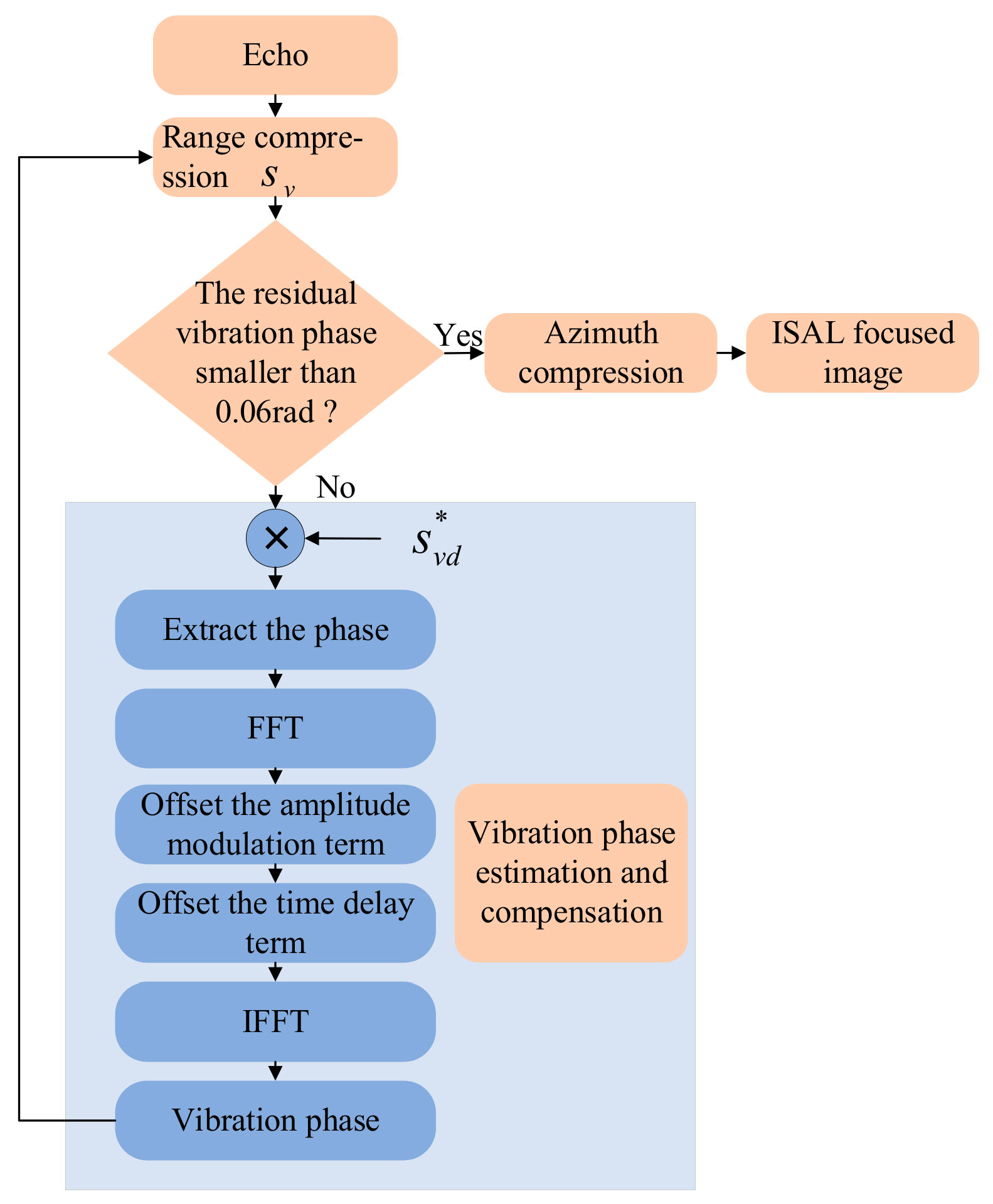
3. Vibration Phase Estimation and Compensation

In this section, the derivation procedure of the vibration phase estimation and the compensation algorithm are presented. According to Equation (10), after the azimuth compression, the amplitudes of the real target and the first couple of ghost targets closest to the real target are ${\sigma }_i{J}_0\left(-\frac{4\pi }{\lambda }{A}_v\right)$ and ${\sigma }_i{J}_1\left(-\frac{4\pi }{\lambda }{A}_v\right)$, respectively.

We define the function $f\left(x\right)$ as follows:

$$f\left(x\right)=20\lg \frac{J_1\left(x\right)}{J_0\left(x\right)}$$

(11)

where $J_0\left(x\right)$ represents the amplitude of the real target, $J_1\left(x\right)$ represents the amplitude of the first couple of ghost targets, $x$ represents $-\frac{4\pi }{\lambda }\widehat{A}$ and $\widehat{A}$ is the amplitude of the vibration phase. Before the vibration phase compensation, $\widehat{A}=A_v$. $f\left(x\right)$ reflects the attenuation of $J_1\left(x\right)$ relative to $J_0\left(x\right)$. In this paper, we define that when $f\left(x\right)\le -30\mathrm{dB}$, the vibration phase can be ignored. From Figure 3, we can know that, if $\left|x\right|\le 0.06rad$, $f\left(x\right)\le -30\mathrm{dB}$. Next, we will reduce the value of $\widehat{A}$ by iteration until $f\left(x\right)\le -30\mathrm{dB}$.

According to Equation (8), when the platform vibrates, the signal phase along the azimuth direction is as follows:

$$\begin{array}{l}\phi =-\frac{4\pi }{\lambda }\left(\left(y_{ip}+x_{ip}\omega t_m\right)+A_v\sin \left({\omega }_v{t}_m+{\phi }_{v0}\right)\right)\\ \begin{array}{c}\end{array}=-\frac{4\pi }{\lambda }\left(y_{ip}+x_{ip}\omega t_m\right)+{\phi }_v\end{array}$$

(12)

where the first term is generated by the rotation of the platform. The second term ${\phi }_v=-\frac{4\pi }{\lambda }{A}_v\sin \left({\omega }_v{t}_m+{\phi }_{v0}\right)$ is the modulation phase introduced by the platform vibration which needs to be suppressed. When $\left|\phi \right|>\pi$, the phase cannot be extracted directly due to the self-coupling. The vibrational phase ${\phi }_v$ needs to be estimated according to the following steps.

Step 1: Conduct delay conjugate multiplication of the data from the same range cell.

We define the range-compressed signal in a range cell as the signal of interest (SoI):

$$s_v=w\left(t_m\right)\cdot \exp \left(-j\frac{4\pi }{\lambda }\left(\left(y_{ip}+x_{ip}\omega t_m\right)+A_v\sin \left({\omega }_v{t}_m+{\phi }_{v0}\right)\right)\right)$$

(13)

where $w\left(t_m\right)$ is the azimuth envelope. After delaying the $s_v$ by $\tau$, we can obtain $s_{vd}$:

$$s_{vd}=w\left(t_m-\tau \right)\exp \left(-j\frac{4\pi }{\lambda }\left(y_{ip}+x_{ip}\omega \left(t_m-\tau \right)+A_v\sin \left({\omega }_v\left(t_m-\tau \right)+{\phi }_{v0}\right)\right)\right)$$

(14)

where $\tau$ is the delay time. Since $w\left(t_m\right)$ changes slowly, we assume that $w\left(t_m-\tau \right)=w\left(t_m\right)$ when $\tau$ is small. Multiplying $s_v$ by $s_{vd}^{*}$, we can obtain the following:

$$\begin{array}{l}{s}_v{s}_{vd}^{*}=w^2\left(t_m\right)\exp \left(-j\frac{4\pi }{\lambda }{x}_{ip}\omega \tau \right)\\ \begin{array}{cc}& \end{array}\hspace{1em}\cdot \exp \left(-j\frac{4\pi }{\lambda }{A}_v\cdot 2\sin \left(\frac{{\omega }_v\tau }{2}\right)\cos \left({\omega }_v\left(t_m-\frac{\tau }{2}\right)+{\phi }_{v0}\right)\right)\end{array}$$

(15)

where * is the conjugate operator and $-\frac{4\pi }{\lambda }{x}_{ip}\omega \tau$ is a constant. It can be seen from Equation (15) that after this delay conjugate multiplication, the phase change caused by the rotation of the platform is eliminated.

Since the constant phase $-\frac{4\pi }{\lambda }{x}_{ip}\omega \tau$ has no relationship with the platform vibration, it can be ignored. Thus, the phase of Equation (15) can be defined as follows:

$${\phi }_v^{\prime }=-\frac{4\pi }{\lambda }{A}_v\cdot 2\sin \left(\frac{{\omega }_v\tau }{2}\right)\cos \left({\omega }_v\left(t_m-\frac{\tau }{2}\right)+{\phi }_{v0}\right)$$

(16)

Step 2: Extract the phase ${\phi }_v^{\prime }$ of $s_v{s}_{vd}^{*}$.

$$\begin{array}{l}{\phi }_v^{\prime }=-\frac{4\pi }{\lambda }{A}_v\cdot 2\sin \left(\frac{{\omega }_v\tau }{2}\right)\cos \left({\omega }_v\left(t_m-\frac{\tau }{2}\right)+{\phi }_{v0}\right)\\ \begin{array}{c}\end{array}=-\frac{4\pi }{\lambda }{A}_v\cdot 2\sin \left(\frac{{\omega }_v\tau }{2}\right)\sin \left({\omega }_v\left(t_m-\frac{\tau }{2}\right)+{\phi }_{v0}+\frac{\pi }{2}\right)\\ \begin{array}{c}\end{array}=-\frac{4\pi }{\lambda }{A}_v\cdot 2\sin \left(\frac{{\omega }_v\tau }{2}\right)\sin \left({\omega }_v\left(t_m-\frac{\tau }{2}+\frac{\pi }{2{\omega }_v}\right)+{\phi }_{v0}\right)\end{array}$$

(17)

Comparing ${\phi }_v^{\prime }$ with the ${\phi }_v$ of Equation (12), we can find that ${\phi }_v^{\prime }$ has an additional amplitude modulation $2\sin \left(\frac{{\omega }_v\tau }{2}\right)$ and a time delay ${\omega }_v\left(-\frac{\tau }{2}+\frac{\pi }{2{\omega }_v}\right)$ along the slow time axis. After offsetting these two parts, we can recover the vibration phase ${\phi }_v$ by using ${\phi }_v^{\prime }$.

Step 3: Offset the amplitude modulation and the time delay terms of ${\phi }_v^{\prime }$.

Take the Fourier transform of ${\phi }_v^{\prime }$:

$$\begin{array}{l}F\left({\phi }_v^{\prime }\right)=-\frac{4\pi }{\lambda }{A}_v\cdot 2\sin \left(\frac{{\omega }_v\tau }{2}\right)\left(\delta \left(f_d+f_v\right)+\delta \left(f_d-f_v\right)\right)\\ \begin{array}{cc}& \end{array}\hspace{1em}\cdot \exp \left(-j2\pi f_d\left(\frac{\tau }{2}-\frac{\pi }{2{\omega }_v}\right)\right)\end{array}$$

(18)

In Equation (18), the last exponential term is the time delay item. After multiplying Equation (18) by $\exp \left(j2\pi f_d\left(\frac{\tau }{2}-\frac{\pi }{2{\omega }_v}\right)\right)/2\sin \left(\frac{{\omega }_v\tau }{2}\right)$, the amplitude modulation and the time delay terms can be removed and we can obtain the following:

$$F\left({\phi }_v^{\prime }\right)=-\frac{4\pi }{\lambda }{A}_v\left(\delta \left(f_d+f_v\right)+\delta \left(f_d-f_v\right)\right)$$

(19)

Step 4: Estimate the vibration phase.

Taking the inverse Fourier transform of Equation (19), we can obtain the estimated value of the vibration phase ${\widehat{\phi }}_v$:

$${\widehat{\phi }}_v=-\frac{4\pi }{\lambda }{A}_v\sin \left({\omega }_v{t}_m+{\widehat{\phi }}_{v0}\right)$$

(20)

where ${\widehat{\phi }}_{v0}$ is the estimated value of ${\phi }_{v0}$. The estimation accuracy of ${\widehat{\phi }}_{v0}$ depends on $\exp \left(j2\pi f_d\left(\frac{\tau }{2}-\frac{\pi }{2{\omega }_v}\right)\right)/2\sin \left(\frac{{\omega }_v\tau }{2}\right)$.

Step 5: Compensate for the vibration phase.

We will compensate for the vibration phase until it is small enough that the influence on the imaging can be ignored.

Multiply $s_v$ by $\exp \left(-j{\widehat{\phi }}_v\right)$ and we can obtain the first compensation signal $s_{c1}$:

$$\begin{array}{l}{s}_{c1}=s_v*\exp \left(-j{\widehat{\phi }}_v\right)\\ \begin{array}{c}\end{array}=w\left(t_m\right)\cdot \exp \left(-j\frac{4\pi }{\lambda }{A}_v\sin \left({\omega }_v{t}_m+{\phi }_{v0}\right)+j\frac{4\pi }{\lambda }{A}_v\sin \left({\omega }_v{t}_m+{\widehat{\phi }}_{v0}\right)\right)\\ \begin{array}{c}\end{array}=w\left(t_m\right)\cdot \exp \left(-j\frac{4\pi }{\lambda }{A}_v\left[\sin \left({\omega }_v{t}_m+{\phi }_{v0}\right)-\sin \left({\omega }_v{t}_m+{\phi }_{v0}-\Delta {\phi }_{v0}\right)\right]\right)\\ \begin{array}{c}\end{array}=w\left(t_m\right)\cdot \exp \left(-j\frac{8\pi }{\lambda }{A}_v\sin \left(\frac{\Delta {\phi }_{v0}}{2}\right)\cos \left({\omega }_v{t}_m+{\phi }_{v0}-\frac{\Delta {\phi }_{v0}}{2}\right)\right)\\ \begin{array}{c}\end{array}=w\left(t_m\right)\cdot \exp \left(-j\frac{8\pi }{\lambda }{A}_v\sin \left(\frac{\Delta {\phi }_{v0}}{2}\right)\cos \left({\omega }_v{t}_m+{\phi }_{v1}\right)\right)\end{array}$$

(21)

where $\Delta {\phi }_{v0}={\phi }_{v0}-{\widehat{\phi }}_{v0}$ and ${\phi }_{v1}={\phi }_{v0}-\frac{\Delta {\phi }_{v0}}{2}$. Then, the residual vibration phase is as follows:

$${\phi }_{c1}=-\frac{8\pi }{\lambda }{A}_v\sin \left(\frac{\Delta {\phi }_{v0}}{2}\right)\cos \left({\omega }_v{t}_m+{\phi }_{v1}\right)$$

(22)

According to Equation (22), compared with the vibration phase ${\phi }_v$, ${\phi }_{c1}$ becomes smaller due to $2\sin \left(\frac{\Delta {\phi }_{v0}}{2}\right)$. If $\left|{\phi }_{c1}\right|>0.06rad$, the impact of ${\phi }_{c1}$ on imaging cannot be ignored. We need to estimate ${\phi }_{c1}$ until it is smaller than 0.06 rad.

The estimation procedure of ${\phi }_{c1}$ is similar to the derivation of Equations (13)–(21). All 5 steps are repeated. After the compensation for ${\phi }_{c1}$, the residual vibration phase is as follows:

$${\phi }_{c2}=\frac{16\pi }{\lambda }{A}_v\sin \left(\frac{\Delta {\phi }_{v0}}{2}\right)\sin \left(\frac{\Delta {\phi }_{v1}}{2}\right)\sin \left({\omega }_v{t}_m+{\phi }_{v2}\right)$$

(23)

where $\Delta {\phi }_{v1}={\phi }_{v1}-{\widehat{\phi }}_{v1}$ and ${\phi }_{v2}={\phi }_{v1}-\frac{\Delta {\phi }_{v1}}{2}$. According to Equation (23), the magnitude of the residual vibration phase is proportional to $4\sin \left(\frac{\Delta {\phi }_{v0}}{2}\right)\sin \left(\frac{\Delta {\phi }_{v1}}{2}\right)$, which indicates that the residual vibration phase will be smaller and smaller by iteration. If the absolute value of residual vibration phase becomes smaller than 0.06 rad, the iteration can be stopped. Otherwise, the above steps 1–5 need to be repeated to compensate for the residual error phase.

There are two points that need to be noted. First, the vibration amplitude should be smaller than a range resolution of ISAL [16]. Second, to avoid the phase self-coupling in Equation (16), the vibration amplitude and the vibration frequency should meet the following condition:

$$\left|-\frac{4\pi }{\lambda }{A}_v\cdot 2\sin \left(\frac{{\omega }_v\tau }{2}\right)\right|<\pi$$

(24)

Set $\tau =1/PRF$, $\sin \left(\frac{{\omega }_v\tau }{2}\right)=\sin \left(\pi \frac{f_v}{PRF}\right)$. Formula (24) can be written as follows:

$$A_v<\frac{\lambda }{8\left|\sin \left(\pi \frac{f_v}{PRF}\right)\right|}$$

(25)

Only when $A_v$ and $f_v$ meet the constraint of Equation (25), the proposed method is valid.

The above compensation of the vibrational phase is based on an isolated scattering point in one range cell. Otherwise, the target contains many scattering points. So, the data in one range cell can be modelled as the first-order Gauss–Markov process [10,18]. Therefore, the algorithm proposed in this paper is also suitable for scenarios with multiple scattering points. The flow chart of this algorithm is shown in Figure 4.

The proposed method can suppress paired echoes without any prior knowledge. After the compensation for the vibration phase, an ISAL image can be obtained by taking the Fourier transform of the compensated signals along the azimuth direction.

4. Experimental Results and Analyses

4.1. Processing Results of Simulated Data

Next, simulations were carried out to verify the proposed methods. Section 4.1.1 shows the simulation results of the fixed amplitude vibration phase compensation. Section 4.1.2 shows the simulation results of the varying amplitude vibration phase compensation. Section 4.1.3 shows the influence of the number of iterations on the estimation accuracy. Section 4.1.4 shows the influence of SNR on the estimation accuracy. Section 4.1.5 shows the compensation results of the data containing multiple vibration components.

The ISAL system parameters, the vibration frequency, the initial vibration phase and the targets in the simulations are all the same in Section 4.1.1, Section 4.1.2, Section 4.1.3 and Section 4.1.4. The simulation parameters are listed in

Table 1. Parameters used in the simulation.

$\lambda$	1550 nm	$\omega$	10°/s
Pulse width	10 us	$R_o$	1 km
Band width	15 GHz	Vibration frequency	5 kHz
Fs	250 MHz	Initial vibration phase	1 rad
PRF	100 kHz	The max vibration amplitude	$\lambda$/10

.

The target distribution is shown in Figure 5. The single scattering point ‘A’ and the scattering point sequence ‘B’ are placed in different range cells. The range-compressed results of ‘A’ and ‘B’ are used as $So{I}_1$ and $So{I}_2$ ($SoI$: the signal of interest), respectively, to compensate for the vibration phase, where ‘B’ is used to verify the vibration phase compensation effectiveness of the proposed method when there are no isolated points in the scene.

For convenience, we define four conditions below.

Condition 1: The amplitude of vibration phase $A_v$ is fixed and the proposed compensation method is based on $So{I}_1$.

Condition 2: The amplitude of vibration phase $A_v$ is fixed and the proposed compensation method is based on $So{I}_2$.

Condition 3: The amplitude of vibration phase $A_v$ is varying and the proposed compensation method is based on $So{I}_1$.

Condition 4: The amplitude of vibration phase $A_v$ is varying and the proposed compensation method is based on $So{I}_2$.

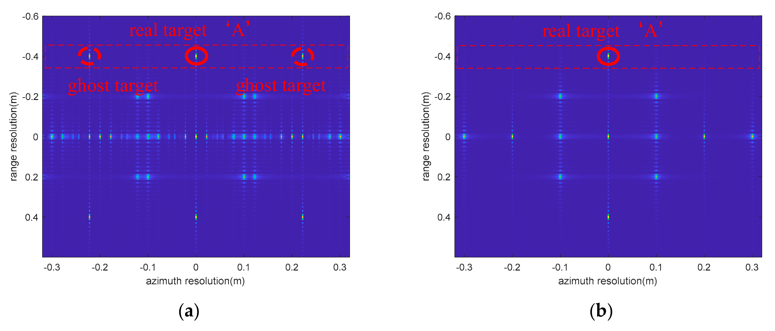
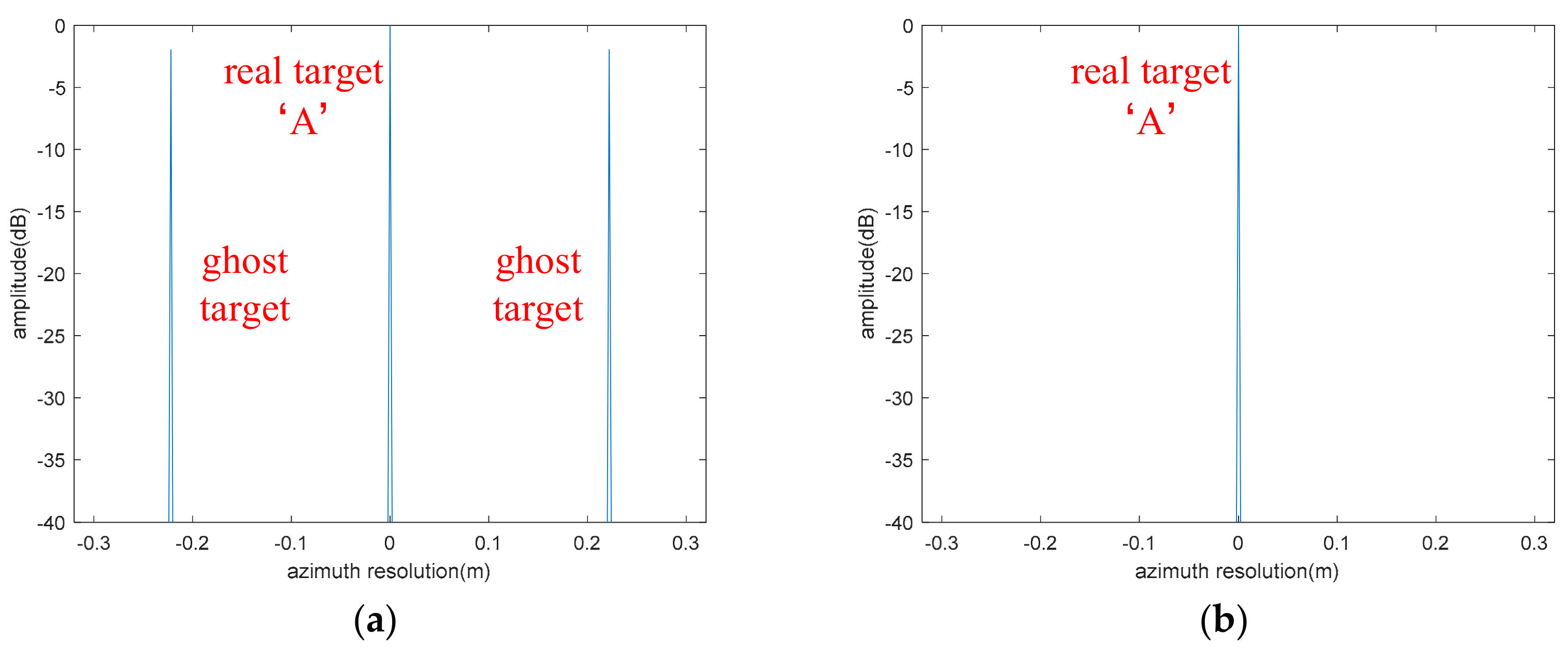
4.1.1. The Compensation Results of Fixed Amplitude Vibration Phase

During echo generation, the fixed amplitude vibration phase shown in Figure 6 is added in the echoes along the azimuth direction. After dechirping, Fourier transformation in the fast time domain and RVP compensation, the range-compressed result can be formatted as shown in Figure 7. We define the range-compressed result of point ‘A’ as $So{I}_1$, and steps 1–5 are repeated to estimate the vibration phase by using $So{I}_1$(condition 1). After three iterations, the vibration phase can be estimated accurately.

The estimation results of the vibration phase under condition 1 are shown in Figure 8. Figure 8b is a partial enlargement of Figure 8a. In Figure 8, the black curve represents the vibration phase added in the echoes, and the other three colored curves represent the estimated vibration phase values obtained by the iterations. It can be seen from Figure 8b that after three iterations, the estimated values are close to the real values. Figure 9a shows the imaging result without vibration phase compensation, in which ghost targets exist along the azimuth direction and the real targets cannot be identified. Figure 9b shows the imaging result after vibration phase compensation using $So{I}_1$. Figure 10a,b show the azimuth profiles of the targets in red dashed boxes in Figure 9a,b, respectively. By comparing Figure 10a,b, we can see that after vibration phase compensation, the ghost targets are compressed.

Next, to verify the vibration phase compensation effectiveness of the proposed method when there are no isolated points in the scene (condition 2), steps 1–5 were repeated to estimate the vibration phase using $So{I}_2$.

The estimated results of the vibration phase are shown in Figure 11. Figure 11b is a partial enlargement of Figure 11a. It can be seen from Figure 11b that the estimated result is close to the real value of the added vibration phase after three iterations. Figure 12a shows the imaging result without vibration phase compensation. Figure 12b shows the imaging result after vibration phase compensation using $So{I}_2$. Figure 13a,b show the azimuth profiles of the targets in red dashed boxes in Figure 12a,b, respectively. By comparing Figure 13a,b, we can see that after vibration phase compensation, the amplitude of the ghost targets dropped from −1.9 to −32.4 dB. Since −32.4 dB < −30 dB, the ghost targets in Figure 13b can be ignored. This result illustrates that the method proposed in this paper is also suitable for scenes without isolated points.

We have analyzed the vibration phase compensation results through the proposed algorithm when the amplitude of vibration phase is fixed. Next, we will analyze the compensation results when the amplitude of vibration phase is varying.

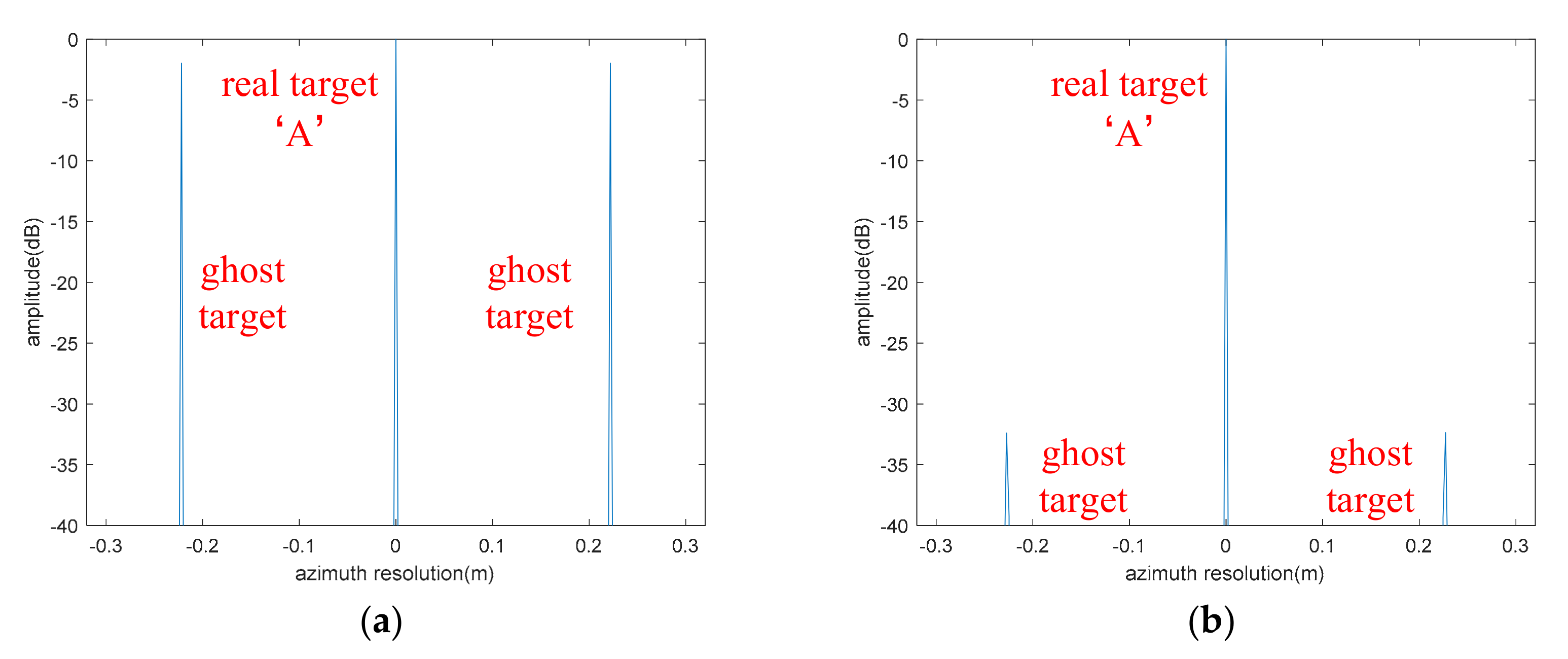
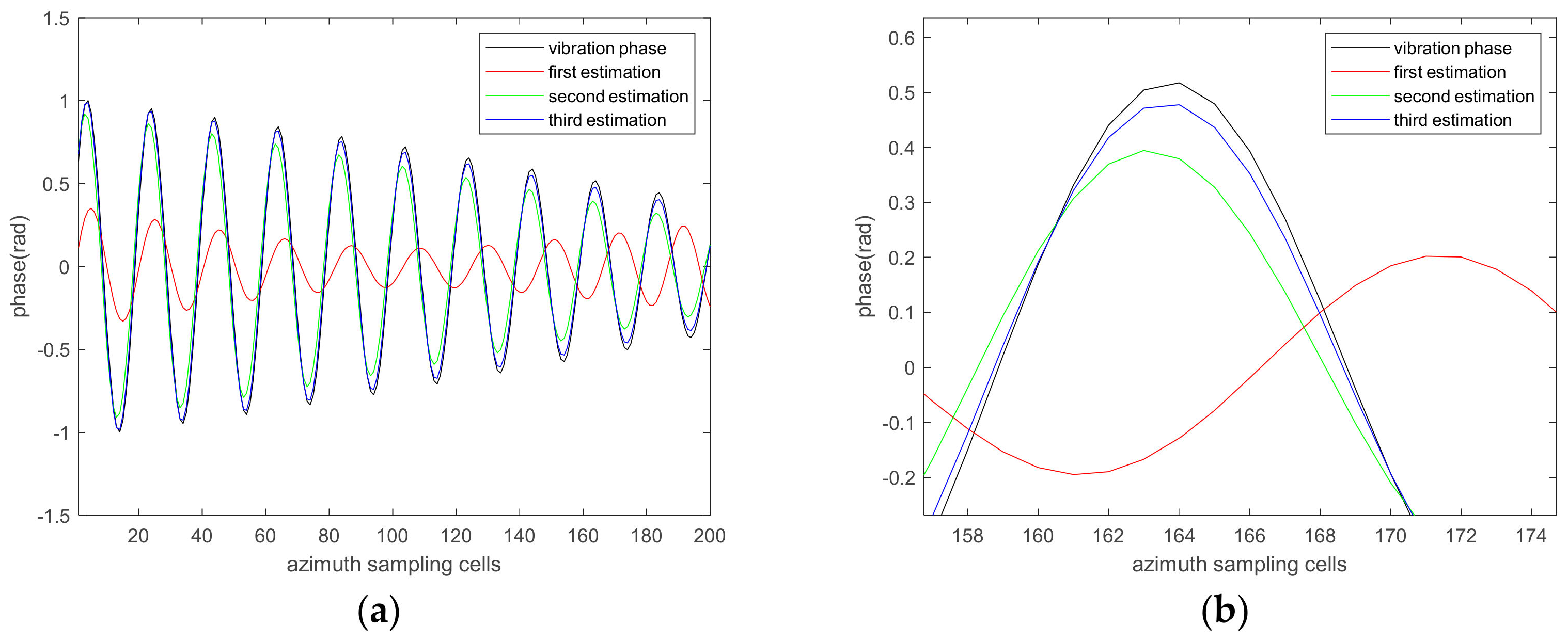
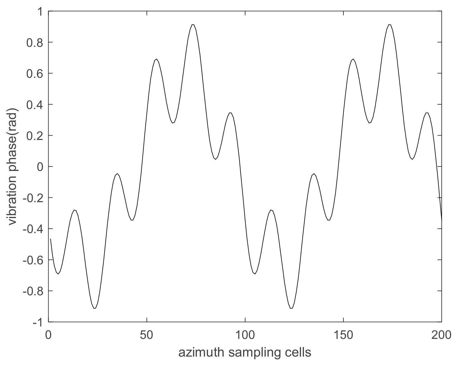
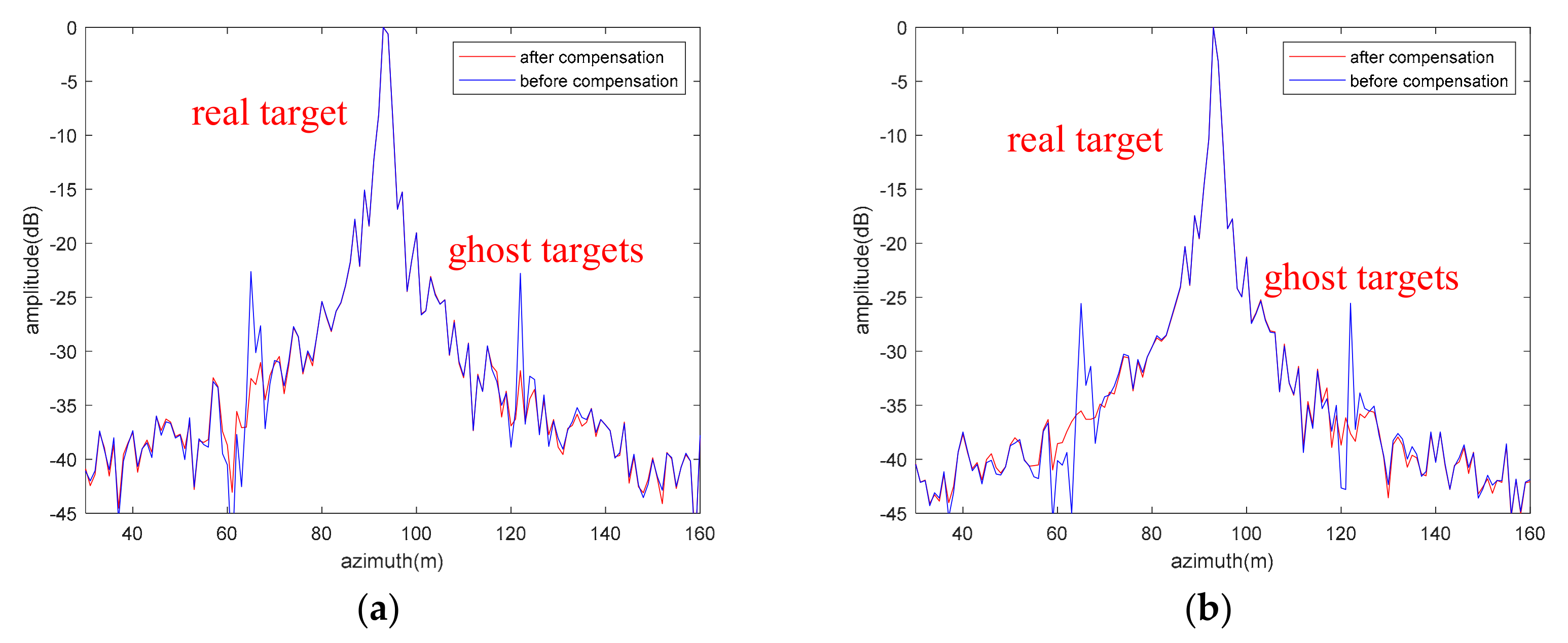
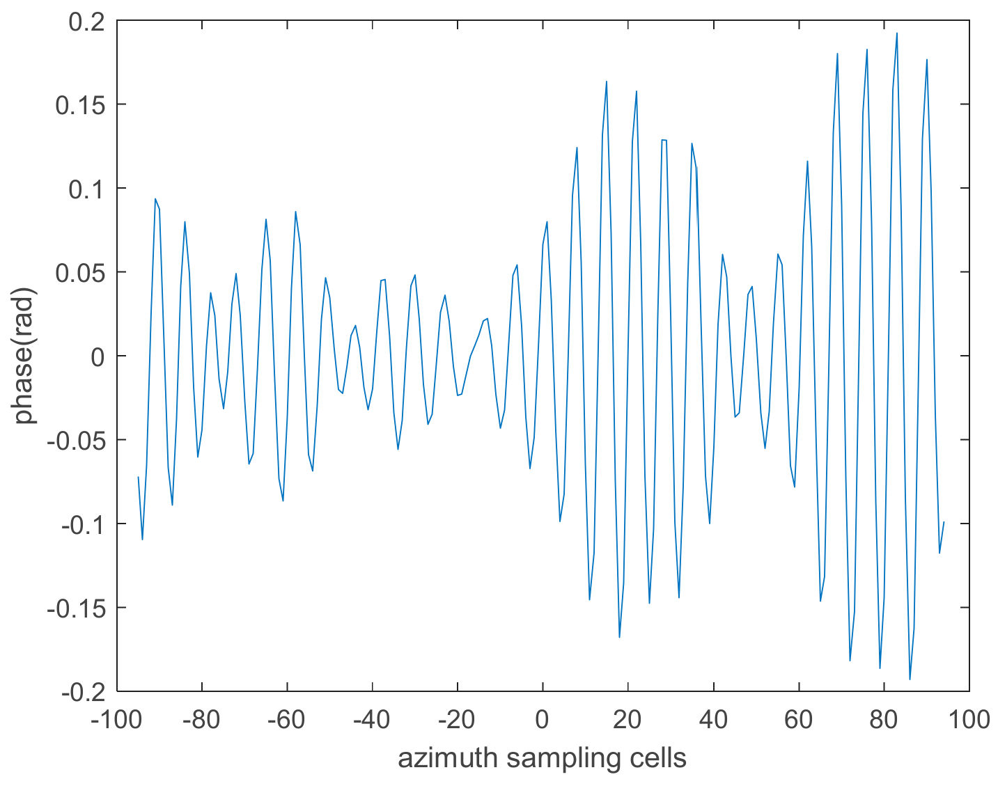
4.1.2. The Compensation Results of Varying Amplitude Vibration Phase

Assuming the varying amplitude vibration phase added in the echoes is the block line in Figure 14, with the target distribution the same as in Figure 5, steps 1–5 were repeated to estimate the vibration phase using $So{I}_1$ (condition 3). The estimated results of the vibration phase are shown in Figure 14. Figure 14b is a partial enlargement of Figure 14a. Figure 15a shows the imaging result without vibration phase compensation. Figure 15b shows the imaging result after vibration phase compensation using $So{I}_1$. Figure 16a,b show the azimuth profiles of the targets in red dashed boxes in Figure 15a,b, respectively. By comparing Figure 16a,b, we can see that, after vibration phase compensation, the ghost targets are compressed.

Next, steps 1–5 were repeated to estimate the vibration phase using $So{I}_2$ (condition 4). The estimated results of the vibration phase are shown in Figure 17. Figure 17b is a partial enlargement of Figure 17a. Figure 18a shows the imaging result without vibration phase compensation. Figure 18b shows the imaging result after vibration phase compensation using $So{I}_2$. Figure 19a,b show the azimuth profiles of targets in the red dashed boxes in Figure 18a,b, respectively. By comparing Figure 19a,b, we can see that, after vibration phase compensation, the amplitude of ghost targets dropped from −9 to −33 dB. Since −33 dB < −30 dB, the ghost targets in Figure 19b can be ignored.

These results demonstrate that the proposed algorithm can estimate fixed and varying amplitude vibration phase based not only on an isolated point but also on multiple scattering points in one range cell. Thus, the proposed algorithm is also suitable for the imaging scenes without isolated points.

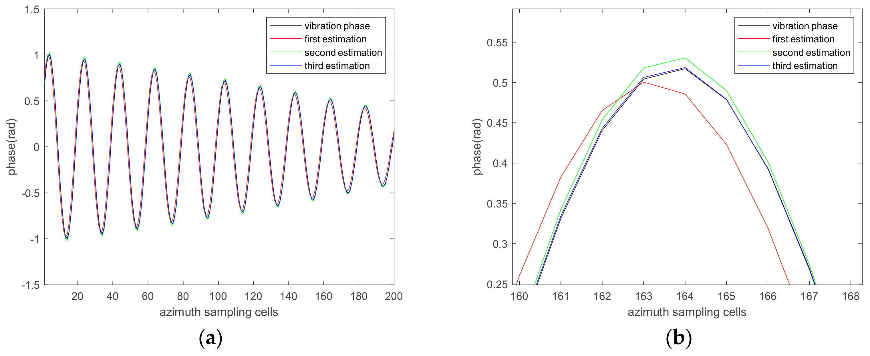
4.1.3. The Influence of the Number of Iterations on the Estimation Accuracy

The influence of the number of iterations on the estimation accuracy is analyzed below. The root mean square error (RMSE) of the estimated values was used to evaluate the estimation accuracy.

$$RMSE=\sqrt{\frac{{\displaystyle \sum _{m=1}^M{\left[{\widehat{\phi }}_v\left(t_m\right)-{\phi }_v\left(t_m\right)\right]}^2}}{M}}$$

(26)

where $M$ and $m$ are the sampling number and the $mth$ sampling point along the azimuth direction, respectively.

Figure 20 shows the RMSE of the estimated vibration phase values with different numbers of iterations. Figure 20a shows the RMSE of the estimated values under condition 1. Figure 20b shows the RMSE of the estimated values under condition 2. Figure 20c shows the RMSE of the estimated values under condition 3. Figure 20d shows the RMSE of the estimated values under condition 4.

From Figure 20, we can see that (1) the RMSE decreases as the number of iterations increases, (2) the estimation result based on the isolated point is better than that based on the point sequence and (3) the RMSE is smaller than 0.06 rad after two or three iterations. In this paper, we operated three iterations for the vibration phase estimation.

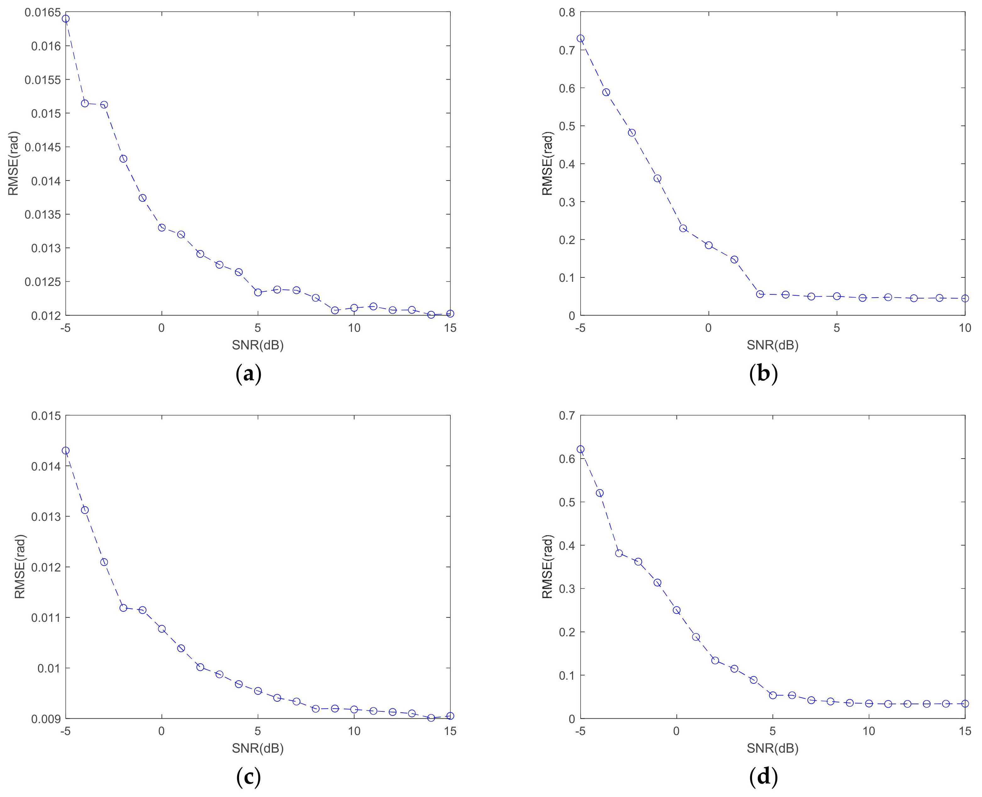
4.1.4. The Influence of SNR on the Estimation Accuracy

To investigate the robustness of our method to SNR, we repeated the simulation under different SNR conditions. Noise was added into the echo by using the awgn function in the simulation. The vibration phase was estimated in three iterations.

To avoid randomness, 100 simulations were performed under conditions 1–4. The average of 100 simulations is shown in Figure 21.

In Figure 21, we note that the amplitude of the RMSE decreases as the SNR increases. When the SNR is higher than −5 dB, the RMSE is smaller than 0.06 rad under conditions 1 and 3. When the SNR is higher than 6 dB, the RMSE is smaller than 0.06 rad under conditions 2 and 4. Generally, the SNR of ISAL images is greater than 10 dB, so the RMSE is smaller than 0.06 rad under conditions 1–4. This phenomenon illustrates that the proposed method has strong robustness to SNR.

4.1.5. The Compensation Results of the Data Containing Multiple Vibration Components

The compensation results of the data containing only one vibration frequency are shown above. Next, the compensation results of the data containing multiple vibration frequencies will be analyzed.

Assume that the echo signal contains two vibration phase components. The vibration parameters used in the simulation are listed in

Table 2. Vibration parameters used in the simulation.

Vibration frequency 1	5 kHz	Vibration frequency 2	1 kHz
Initial vibration phase 1	1 rad	Initial vibration phase 2	0.5 rad
Vibration amplitude 1	$\lambda$/40	Vibration amplitude 2	$\lambda$/20

.

During echo generation, the vibration phase shown in Figure 22 is added in the echoes. It can be seen from Figure 22 that the amplitude of vibration phase $A_v$ is varying.

We define the range-compressed result of point ‘A’ as $So{I}_1$, and steps 1–5 were repeated to estimate these two vibration phase components. Figure 23 is the imaging result without compensation. Figure 24a,b show the imaging result after compensating vibration component 1 and vibration component 2, respectively.

Next, we define the range-compressed result of point ‘B’ as $So{I}_2$, and steps 1–5 were repeated to estimate these two vibration phase components. Figure 25a,b are the imaging result after compensating vibration component 1 and vibration component 2, respectively. These results demonstrate that the proposed algorithm can estimate the vibration phase containing multiple frequencies.

4.2. Processing Result of Real Data

Real data of 1550 nm, 4 G bandwidth, 50 kHz PRF, an angular velocity of 10°/s and a distance of 1 km were processed. The transmission signal was an LFM signal, and the reception mode was dechirping reception.

Figure 26 shows an optical picture of targets placed on the turntable. We will analyze the vibration phase compensation results by using the proposed method when the targets are static and rotating.

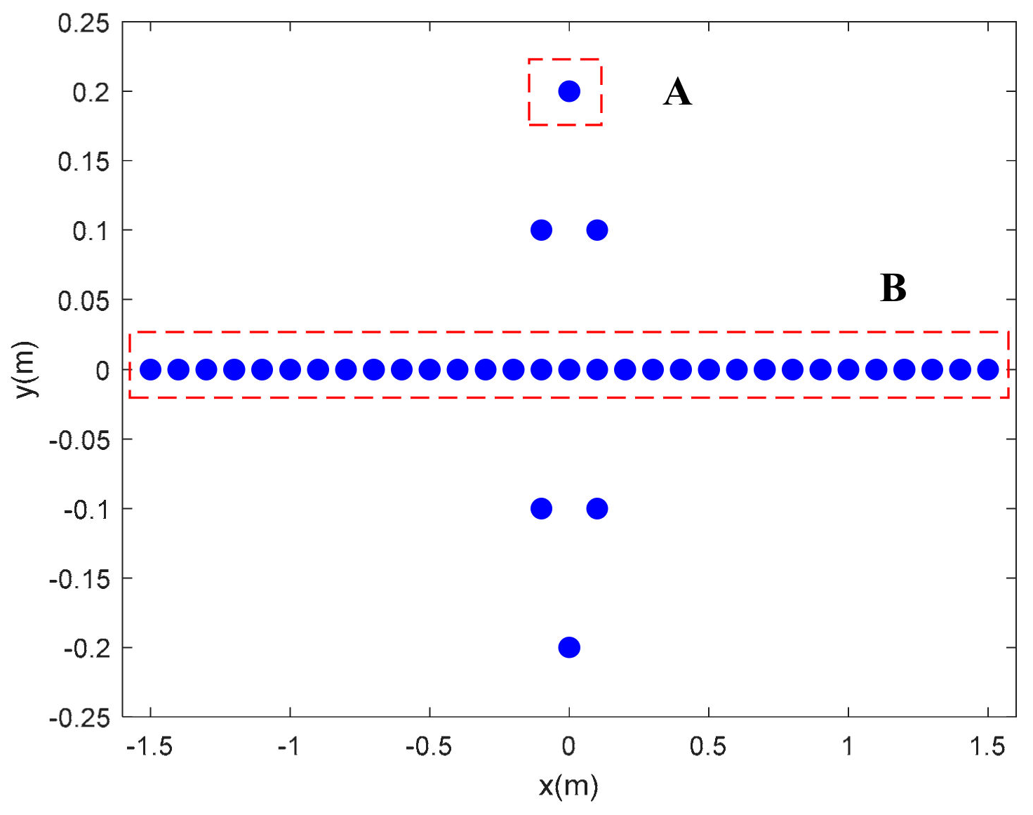
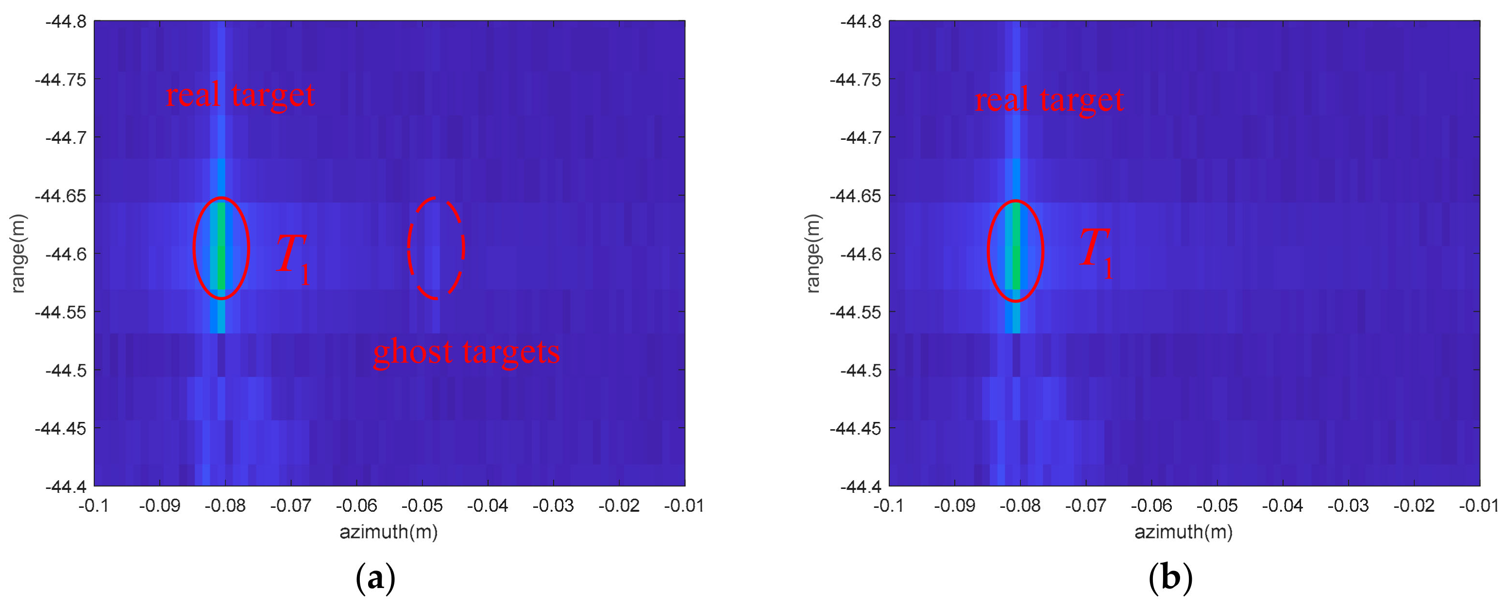
4.2.1. Stationary Point Targets

During echo generation, the turntable was static. After dechirping, Fourier transform in the fast time domain and RVP compensation, the range-compressed result was obtained and is shown in Figure 27. The phases of the delay conjugate multiplication of the range-compressed date in the 1312 and 1317 range cell of Figure 27 are shown in Figure 28. Figure 28 shows that sinusoidal modulation exists in the phase along the azimuth direction.

We defined the range-compressed data in row 1312 as $SoI$; then, we estimated the vibration phase using the proposed method. After three iterations, we obtained the estimated vibration phase shown in Figure 29. From Figure 29, we can see that the amplitude of the vibration phase is varying. Figure 30a is the imaging result of two targets without vibration phase compensation, where $T_1$ and $T_2$ are the real point targets, and the other ones on the left and right of $T_1$ and $T_2$ are ghost targets. Figure 30b is the imaging result of two targets after vibration phase compensation, in which the ghost targets are suppressed. Figure 31a,b are the azimuth profiles of target $T_1$ and target $T_2$, respectively.

It can be seen from Figure 31a,b that after the vibration phase compensation, the left ghost target of $T_1$ dropped from −22.62 to −32.42 dB and the right ghost target of $T_1$ dropped from −22.79 to −31.86 dB. The left ghost target of $T_2$ dropped from −22.58 to −35.18 dB and the right ghost target of $T_2$ dropped from −25.56 to −37.98 dB. These results indicate that the ghost targets were suppressed using the proposed method.

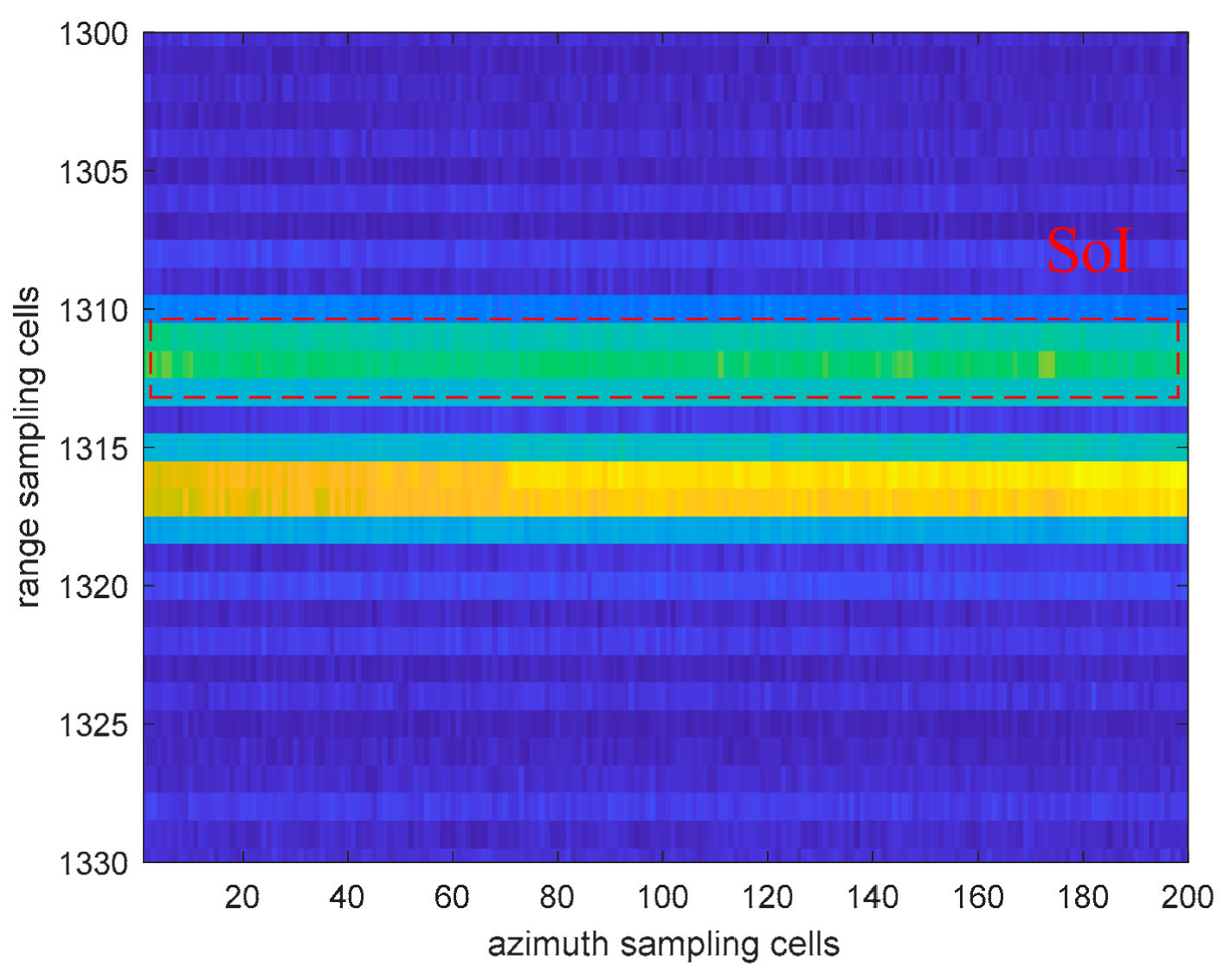
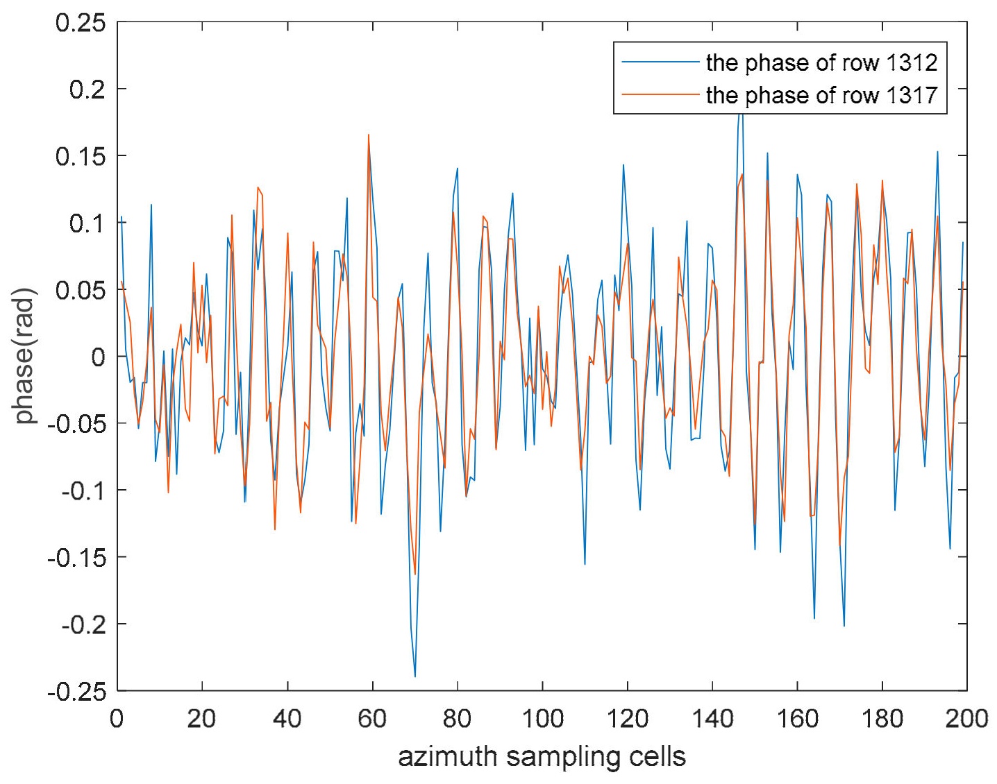
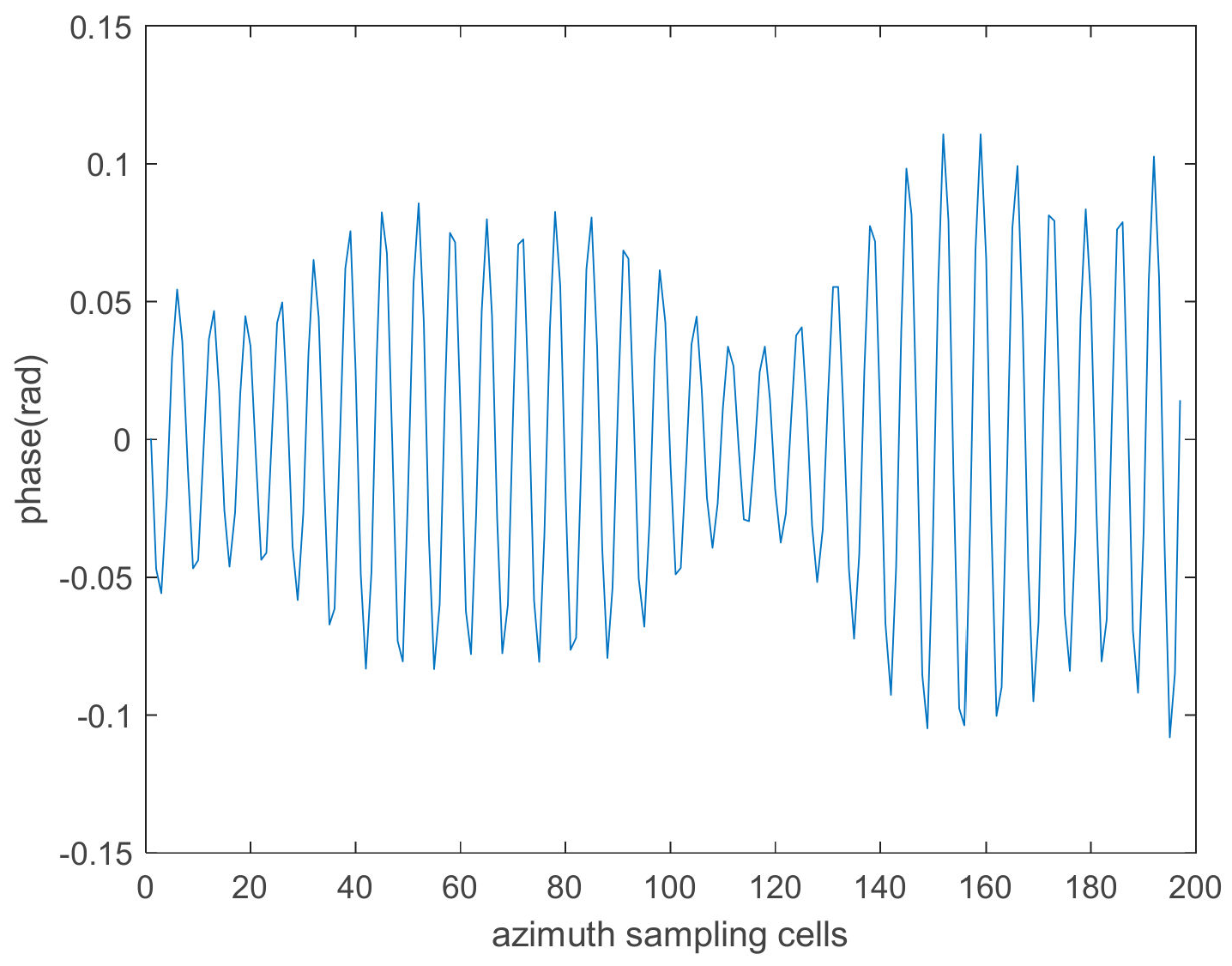
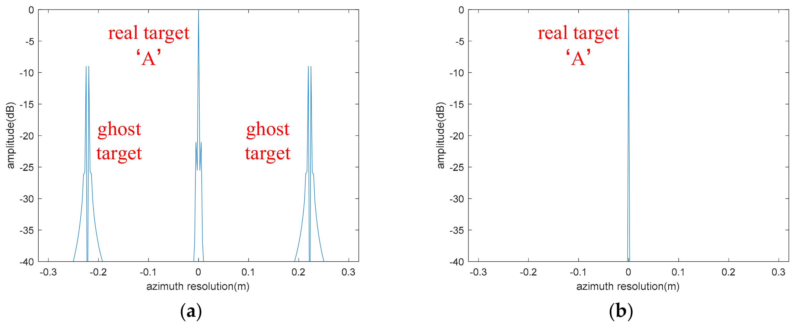
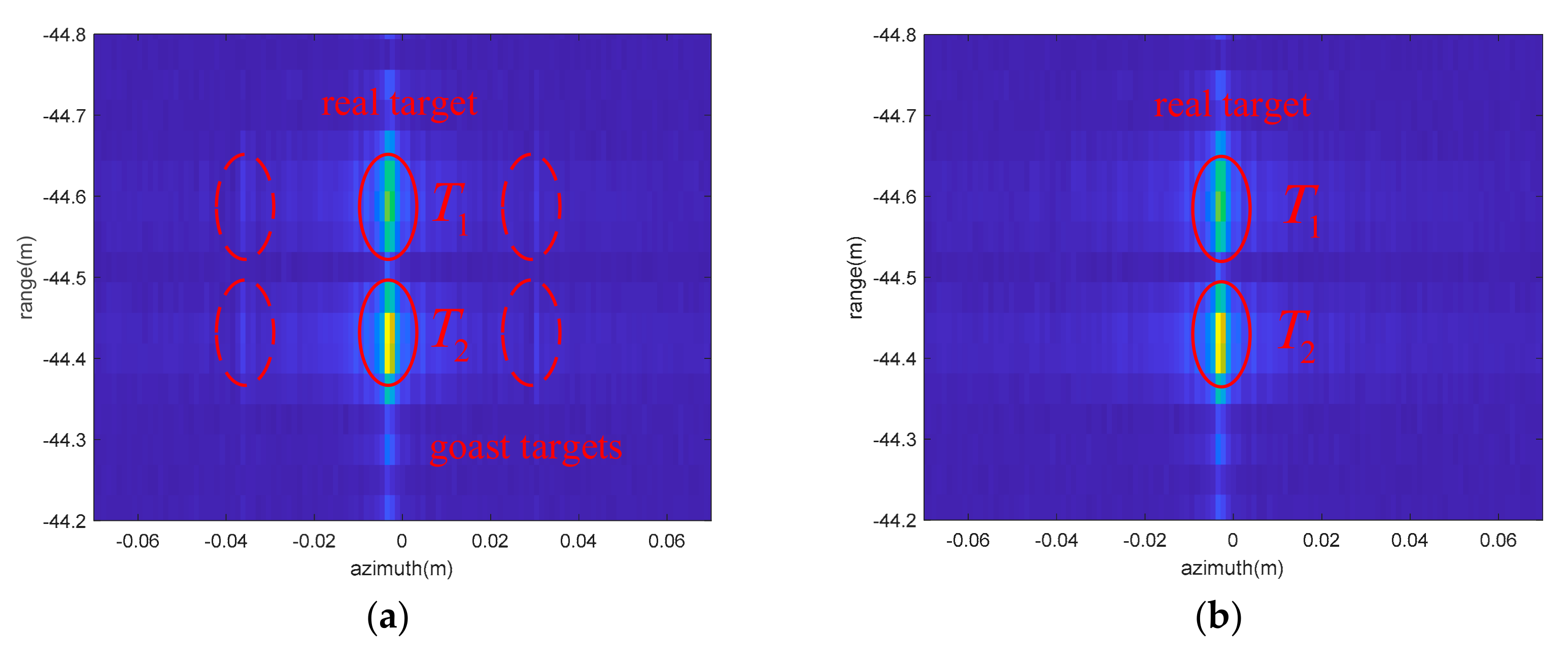
4.2.2. Rotating Point Targets

Figure 32 is the imaging result of two points with platform vibration when the turntable rotated. The target $T_1$ and the target $T_2$ in Figure 32 are the real point targets, and the other ones on the left and right of them are the ghost targets formed by the platform vibration. We also defined the data in row 1312 as $SoI$ and estimated the vibration phase using the proposed method. Figure 33 shows the estimated result of the vibration phase, whose amplitude is varying. Figure 34a,b are the imaging results of target $T_1$ without and with vibration phase compensation. Figure 35a,b are the imaging results of target $T_2$ without and with vibration phase compensation. The azimuth profiles of these two point targets without and with compensation are shown in Figure 36a,b.

It can be seen from Figure 36 that after the vibration phase compensation, the right ghost target of $T_1$ dropped from −24.51 dB to −37.41 dB, and the right ghost target of $T_2$ dropped from −27.67 dB to −39.62 dB. The real data results show that the algorithm proposed in this paper can suppress ghost targets without introducing new phase error and without broadening the main lobe of targets.

5. Discussion

A vibration phase compensation method based on the delay conjugate multiplication of echoes is proposed in this paper, which can suppress paired echoes under the condition of varying amplitude vibrations for a single-channel transceiver system transmitting LFM signals.

According to the Jacobi–Anger identity, we defined the function $f\left(x\right)$, which reflects the amplitude attenuation of the real target relative to the first couple of ghost targets. We think that when $f\left(x\right)\le -30\mathrm{dB}$, the vibration phase can be ignored. In this paper, we reduced the values of the vibration phase by iteration until $f\left(x\right)\le -30\mathrm{dB}$. The detailed steps are given in Section 3.

The processing results in Section 4 demonstrate the following:

(1)

The proposed algorithm can estimate the fixed and varying amplitude vibration phase.

(2)

The proposed algorithm is suitable for imaging scenes both with and without isolated points.

(3)

The residual vibration phase decreases as the number of iterations increases. In this paper, we operated three iterations for the vibration phase estimation.

(4)

Generally, the SNR of ISAL images is greater than 10 dB, so the proposed method has strong robustness to SNR.

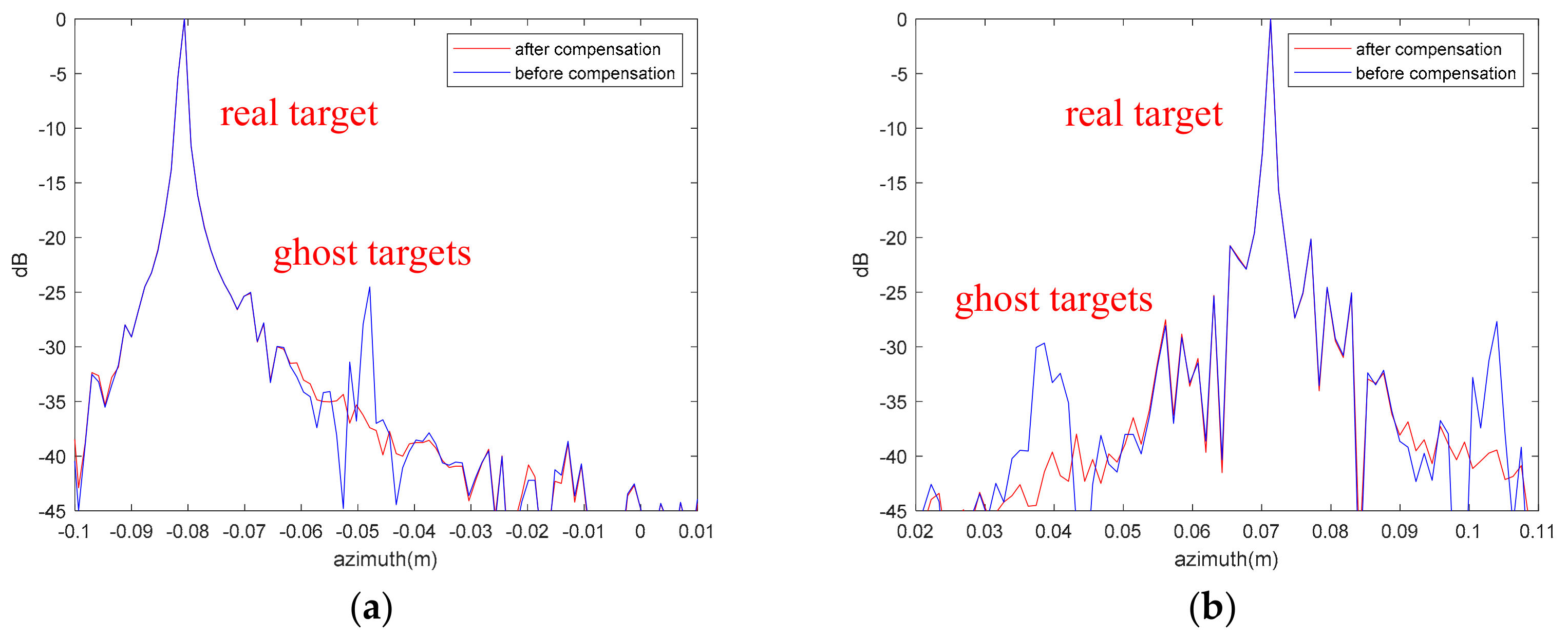
(5)

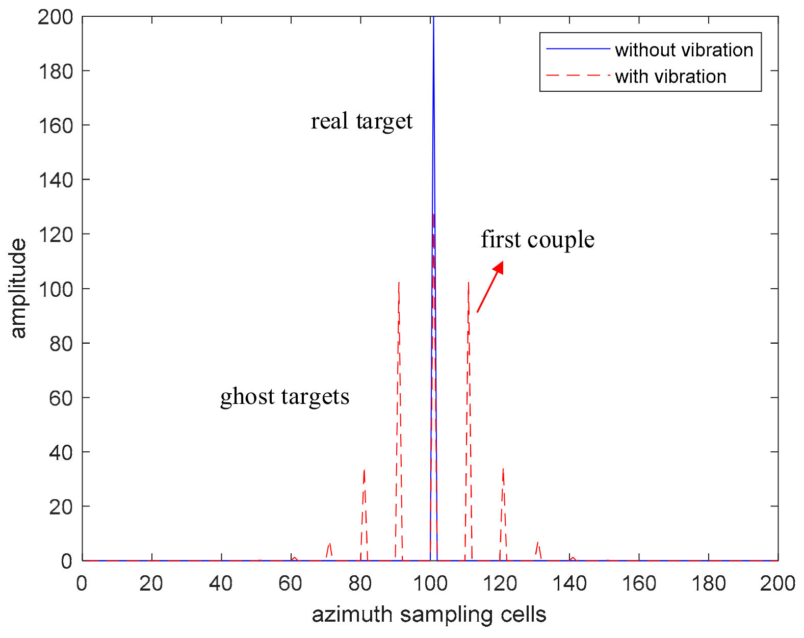
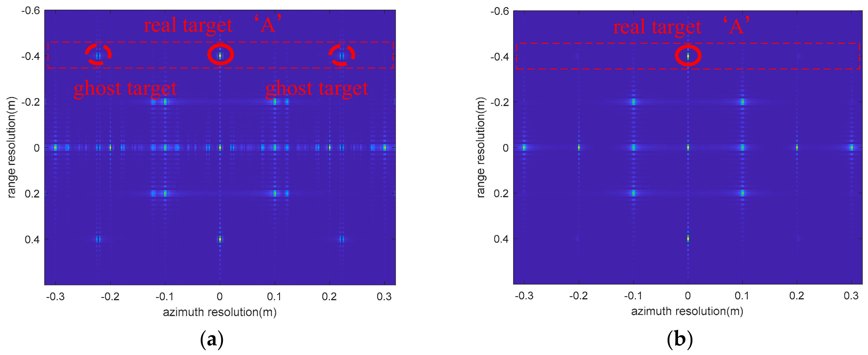
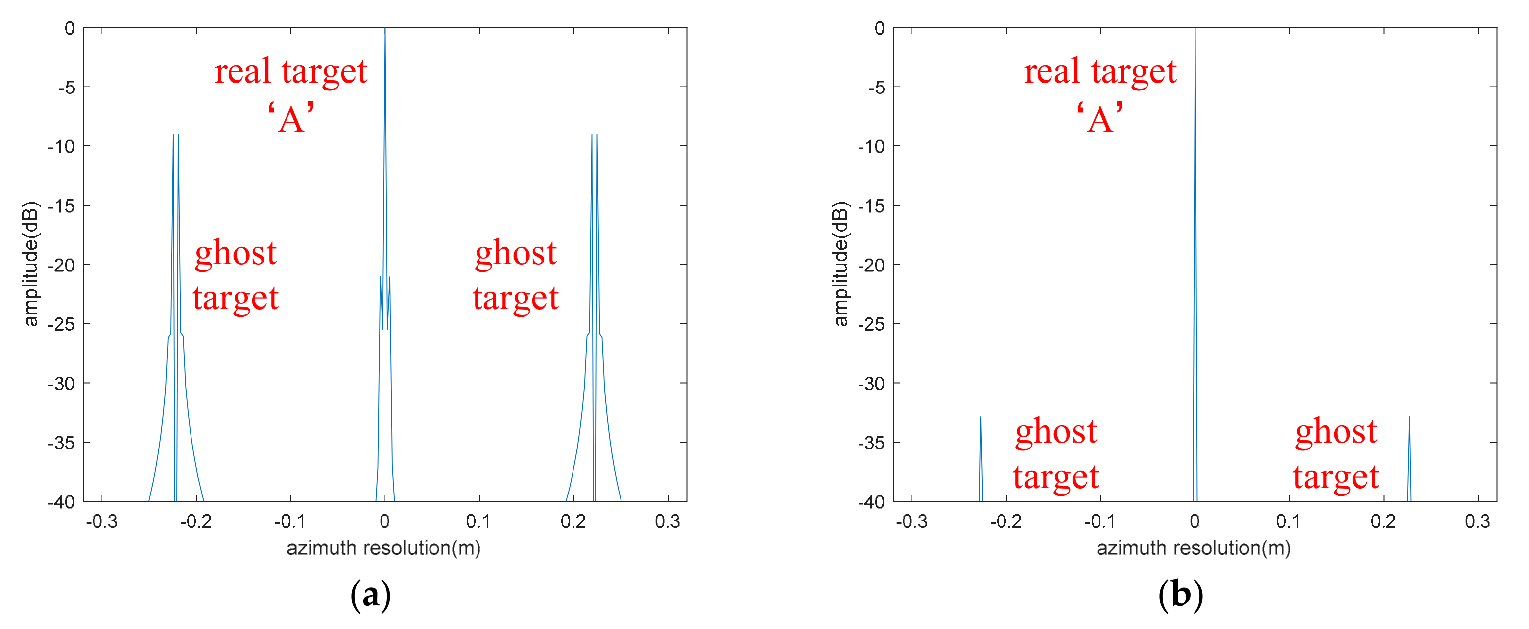
The proposed algorithm can suppress ghost targets without introducing new phase error and without broadening the main lobe of targets.

These observations are meaningful in ISAL imaging, target identification and classification.

6. Conclusions

To suppress the paired echoes generated by the platform vibration in ISAL imaging, this paper proposes an iterative algorithm to estimate and compensate for the vibration phase. The results show that the proposed algorithm can estimate not only the fixed but also varying vibration phase. Furthermore, the proposed algorithm can work without prior knowledge and will not introduce new phase errors, and it is suitable for the imaging scenes with no isolated points.

References

1. Beck, S.M.; Buck, J.R.; Buell, W.F.; Dickinson, R.P.; Kozlowski, D.A.; Marechal, N.J.; Wright, T.J. Synthetic-aperture imaging laser radar: Laboratory demonstration and signal processing. Appl. Opt. 2005, 44, 7621–7629. [Google Scholar] [CrossRef] [PubMed]
2. Guo, L.; Yin, H.F.; Zhou, Y.; Sun, J.F.; Zeng, X.D.; Tang, Y.; Xing, M.D. A novel sidelobe-suppression algorithm for airborne synthetic aperture imaging ladar. Opt. Laser Technol. 2019, 111, 714–719. [Google Scholar] [CrossRef]
3. Huang, Y.; Song, S.; Xu, W.; Hu, Y. Real-time inverse synthetic aperture ladar system based on continuous m-sequence phase modulation. Laser Optoelectron. Prog. 2021, 54, 072801. [Google Scholar] [CrossRef]
4. Liang, G.; Yu, T.; Meng-dao, X.; Zheng, B. Experimentation system of synthetic aperture imaging lidar. J. Electron. 2009, 26, 433–443. [Google Scholar] [CrossRef]
5. Crouch, S.; Barber, Z.W. Laboratory demonstrations of interferometric and spotlight synthetic aperture ladar techniques. Opt. Express 2012, 20, 24237–24246. [Google Scholar] [CrossRef] [PubMed]
6. Lu, Z.Y.; Zhou, Y.; Sun, J.F.; Luan, Z.; Wang, L.J.; Xu, Q.; Li, G.Y.; Zhang, G.; Liu, L.R. Airborne down-looking synthetic aperture imaging ladar field experiment and its flight testing. Chin. J. Lasers 2017, 44, 0110001. [Google Scholar] [CrossRef]
7. Li, G.Z.; Wang, N.; Wang, R.; Zhang, K.S.; Wu, Y.R. Imaging method for airborne SAL data. Electron. Lett. 2017, 53, 351–353. [Google Scholar] [CrossRef]
8. Chen, V.; Li, F.; Ho, S.S.; Wechsler, H. Micro-doppler effect in radar: Phenomenon, model, and simulation study. IEEE Trans. Aerosp. Electron. Syst. 2006, 42, 2–21. [Google Scholar] [CrossRef]
9. Molchanov, P.; Astola, J.; Egiazarian, K.; Totsky, A. On Micro-Doppler Period Estimation. In Proceedings of the 2013 19th International Conference on Control Systems and Computer Science, Bucharest, Romania, 29–31 May 2013; pp. 325–330. [Google Scholar] [CrossRef]
10. Gao, Y.; Zhang, Z.; Xing, M.; Zhang, Y.; Li, Z. Paired echo suppression algorithm in helicopter-borne SAR imaging. IET Radar Sonar Navig. 2017, 11, 1605–1612. [Google Scholar] [CrossRef]
11. Wang, Y.; Wang, Z.; Zhao, B.; Xu, L. Compensation for High-Frequency Vibration of Platform in SAR Imaging Based on Adaptive Chirplet Decomposition. IEEE Geosci. Remote Sens. Lett. 2016, 13, 792–795. [Google Scholar] [CrossRef]
12. Wang, Q.; Pepin, M.; Wright, A.; Dunkel, R.; Atwood, T.; Santhanam, B.; Gerstle, W.; Doerry, A.W.; Hayat, M.M. Reduction of vibration-induced artifacts in synthetic aperture radar imagery. IEEE Trans. Geosci. Remote Sens. 2014, 52, 3063–3073. [Google Scholar] [CrossRef] [Green Version]
13. Wang, Q.; Pepin, M.; Beach, R.J.; Dunkel, R.; Atwood, T.; Santhanam, B.; Gerstle, W.; Doerry, A.W.; Hayat, M.M. SAR-Based Vibration Estimation Using the Discrete Fractional Fourier Transform. IEEE Trans. Geosci. Remote Sens. 2012, 50, 4145–4156. [Google Scholar] [CrossRef] [Green Version]
14. Setlur, P.; Amin, M.; Thayaparan, T. Micro-Doppler signal estimation for vibrating and rotating targets. In Proceedings of the Eighth International Symposium on Signal Processing and Its Applications, Sydney, NSW, Australia, 28–31 August 2005; pp. 639–642. [Google Scholar]
15. Zhang, Y.; Sun, J.; Lei, P.; Hong, W. SAR-based paired echo focusing and suppression of vibrating targets. IEEE Trans. Geosci. Remote Sens. 2014, 52, 7593–7605. [Google Scholar] [CrossRef]
16. Hu, X.; Li, D.J. Vibration phases estimation based on multi-channel interferometry for ISAL. Appl. Opt. 2018, 57, 6481–6490. [Google Scholar] [CrossRef] [PubMed]
17. Wang, R.; Wang, B.; Xiang, M.; Li, C.; Wang, S. Vibration compensation method based on instantaneous ranging model for triangular FMCW ladar signals. Opt. Express 2021, 29, 15918–15939. [Google Scholar] [CrossRef] [PubMed]
18. Ash, J.; Ertin, E.; Potter, L.; Zelnio, E. Wide-angle synthetic aperture radar imaging: Models and algorithms for anisotropic scattering. IEEE Signal Processing Mag. 2014, 31, 16–26. [Google Scholar] [CrossRef]
Figure 1. ISAL turntable imaging geometry.
Remotesensing 14 01122 g001
Figure 2. The azimuth compression results with or without platform vibration.
Remotesensing 14 01122 g002
Figure 3. The function curve of f x .
Remotesensing 14 01122 g003
Figure 4. The flow chart of vibration phase estimation and compensation algorithm.
Remotesensing 14 01122 g004
Figure 5. Target distribution.
Remotesensing 14 01122 g005
Figure 6. Fixed amplitude vibration phase.
Remotesensing 14 01122 g006
Figure 7. The range-compressed results.
Remotesensing 14 01122 g007
Figure 8. (a) Vibration phase and its estimated values under condition 1. (b) Partial enlargement of (a).
Remotesensing 14 01122 g008
Figure 9. Imaging results without (a) and with (b) compensation under condition 1.
Remotesensing 14 01122 g009
Figure 10. Azimuth profiles of targets in the red dashed boxes in Figure 9. (a) Without compensation and (b) with compensation.
Remotesensing 14 01122 g010
Figure 11. (a) Vibration phase and its estimated value under condition 2. (b) Partial enlargement of (a).
Remotesensing 14 01122 g011
Figure 12. Imaging results without (a) and with (b) compensation under condition 2.
Remotesensing 14 01122 g012
Figure 13. Azimuth profile of targets in the red dashed boxes in Figure 12. (a) Without compensation and (b) with compensation.
Remotesensing 14 01122 g013
Figure 14. (a) Vibration phase and its estimated value under condition 3. (b) Partial enlargement of (a).
Remotesensing 14 01122 g014
Figure 15. Imaging results without and with compensation under condition 3. (a) Without compensation and (b) with compensation.
Remotesensing 14 01122 g015
Figure 16. Azimuth profiles of targets in the red dashed boxes in Figure 15. (a) Without compensation and (b) with compensation.
Remotesensing 14 01122 g016
Figure 17. (a) Vibration phase and its estimated value under condition 4. (b) Partial enlargement of (a).
Remotesensing 14 01122 g017
Figure 18. Imaging results without (a) and with (b) compensation under condition 4.
Remotesensing 14 01122 g018
Figure 19. Azimuth profile of targets in the red dashed boxes in Figure 18. (a) Without compensation and (b) with compensation.
Remotesensing 14 01122 g019
Figure 20. The RMSE of the estimated vibration phase values with different numbers of iterations: (a) Under condition 1; (b) under condition 2; (c) under condition 3; (d) under condition 4.
Remotesensing 14 01122 g020aRemotesensing 14 01122 g020b
Figure 21. The RMSE of the estimated vibration phase values with different SNRs: (a) Under condition 1; (b) under condition 2; (c) under condition 3; (d) under condition 4.
Remotesensing 14 01122 g021
Figure 22. Vibration phase added in the echoes.
Remotesensing 14 01122 g022
Figure 23. (a) The imaging result without compensation; (b) azimuth profile of targets in the red dashed boxes.
Remotesensing 14 01122 g023
Figure 24. The imaging result after compensating vibration component 1 (a) and compensating vibration component 2 (b) using S o I 1 .
Remotesensing 14 01122 g024
Figure 25. The imaging result after compensating vibration component 1 (a) and compensating vibration component 2 (b) using S o I 2 .
Remotesensing 14 01122 g025
Figure 26. Optical picture of targets.
Remotesensing 14 01122 g026
Figure 27. Range compression result of echo.
Remotesensing 14 01122 g027
Figure 28. The phase of delay conjugate multiplication.
Remotesensing 14 01122 g028
Figure 29. Estimated vibration phase.
Remotesensing 14 01122 g029
Figure 30. Imaging results (a) without compensation and (b) with compensation.
Remotesensing 14 01122 g030
Figure 31. Azimuth profiles of T 1 (a) and T 2 (b) in Figure 30.
Remotesensing 14 01122 g031
Figure 32. Imaging results without compensation.
Remotesensing 14 01122 g032
Figure 33. Estimated vibration phase.
Remotesensing 14 01122 g033
Figure 34. Partial enlargement of T 1 (a) without compensation and (b) with compensation.
Remotesensing 14 01122 g034
Figure 35. Partial enlargement of T 2 (a) without compensation and (b) with compensation.
Remotesensing 14 01122 g035
Figure 36. Azimuth profiles of T 1 (a) and T 2 (b) without and with compensation.
Remotesensing 14 01122 g036