Article

Improved U-Net Remote Sensing Classification Algorithm Based on Multi-Feature Fusion Perception

1
School of Electrical, Electronic and Computer Science, Guangxi University of Science and Technology, Liuzhou 545006, China
2
National Satellite Meteorological Center of China Meteorological Administratio, Beijing 100089, China
*
Author to whom correspondence should be addressed.
Remote Sens. 2022, 14(5), 1118; https://doi.org/10.3390/rs14051118
Submission received: 9 February 2022 / Revised: 20 February 2022 / Accepted: 22 February 2022 / Published: 24 February 2022
(This article belongs to the Special Issue Advanced Earth Observations of Forest and Wetland Environment)

Abstract

:
The selection and representation of remote sensing image classification features play crucial roles in image classification accuracy. To effectively improve the classification accuracy of features, an improved U-Net network framework based on multi-feature fusion perception is proposed in this paper. This framework adds the channel attention module (CAM-UNet) to the original U-Net framework and cascades the shallow features with the deep semantic features, replaces the classification layer in the original U-Net network with a support vector machine, and finally uses the majority voting game theory algorithm to fuse the multifeature classification results and obtain the final classification results. This study used the forest distribution in Xingbin District, Laibin City, Guangxi Zhuang Autonomous Region as the research object, which is based on Landsat 8 multispectral remote sensing images, and, by combining spectral features, spatial features, and advanced semantic features, overcame the influence of the reduction in spatial resolution that occurs with the deepening of the network on the classification results. The experimental results showed that the improved algorithm can improve classification accuracy. Before the improvement, the overall segmentation accuracy and segmentation accuracy of the forestland increased from 90.50% to 92.82% and from 95.66% to 97.16%, respectively. The forest cover results obtained by the algorithm proposed in this paper can be used as input data for regional ecological models, which is conducive to the development of accurate and real-time vegetation growth change models.

1. Introduction

Remote sensing technology plays an important role in the fields of crop monitoring, geological investigation, and precision agriculture [1,2,3]. Carbon balance has always been a topic of concern worldwide, and forest resources largely contribute to the global carbon balance, so it is necessary to accurately monitor the dynamic changes of forest resources [4]. However, the use of remote sensing images to identify different features with high accuracy, and to classify and count various kinds of feature information, is a popular and difficult research point in remote sensing information extraction. The essence of the image-specific target segmentation challenge in remote sensing is to construct a target feature space and its mapping model. The current mainstream remote sensing classification methods mainly include traditional machine learning methods and semantic segmentation methods based on deep learning, and the corresponding algorithms will be introduced in the following section.

Related Work

Traditional remote sensing image classification methods, such as the k-means clustering method [5], watershed algorithm [6], and active contour model [7], manually extract feature values corresponding to targets in a remote sensing image space to form a feature space and construct a mapping model from the feature space to the target space. However, the mapping model from the feature space to the target space is a high-dimensional, strongly nonlinear relationship, which is difficult to implement using manual methods. Thus, some scholars have proposed learning-based remote sensing image segmentation methods to establish mapping models through sample learning. Dong et al. [8] introduced a number of single complementary features combined with back propagation (BP) neural networks to improve the accuracy of single tree detection. Sun et al. [9] introduced a Mahalanobis Distance kernel to improve the classification performance of support vector machines (SVMs) for remote sensing images. Li et al. [10] combined spectral features, vegetation indices, texture features, and topography to establish a random forest model to identify the forest types in the HeiLongJiang Cap Mountains. The aforementioned early remote sensing image classification methods mainly use the low-level features of images for model training. However, there is an insufficient utilization of feature information, which needs to be improved for feature refinement classification, and it is difficult to distinguish complex feature types.
The semantic segmentation method based on deep learning is applied to remote sensing image classification and shows good performance. Deep convolutional neural networks (CNNs) can automatically extract different classes of features in remote sensing images [11,12,13,14,15] with good accuracy. Kussual et al. [16] proposed a multi-level deep learning method for land cover and crop type classification using multitemporal multisource satellite images to classify 11 classes of crops, such as wheat, corn, and sunflower. Alshehhi et al. [17] combined low-level features with high-level semantic features extracted by CNNs to classify roads and buildings in cities. Csillik et al. [18] used CNNs to identify citrus trees from UAV images. Nowadays, deep neural networks are highly capable of image feature extraction, and extreme learning machines (ELMs) and SVMs, which are traditional linear classifiers, have strong capabilities in classification. Therefore, the use of ELMs or SVMs in classification has been proposed to improve accuracy after the feature extraction of CNNs is in effect. Wang et al. [19] proposed a CNN and ELM fusion method, where a CNN is used for feature extraction and an ELM is used as a classifier. Cao et al. [20] designed a combined CNN and SVM method to identify ships. Meng et al. [21] used a CNN to classify remote sensing images of wetlands and compared it with methods based on spectral SVM and texture and spectral SVM. Sun et al. [22] designed a seven-layer CNN structure, trained the samples with the CNN, and then used an SVM to classify remote sensing images and tested them with volcanic ash clouds. The aforementioned studies used CNNs for feature extraction and used ELM and SVM classifiers to improve classification accuracy. However, these studies only extracted the features of one layer and did not consider the features of different layers together. Long et al. [23] proposed a fully convolutional network (FCN) model. The FCN model replaces the fully connected layers in a CNN with convolutional layers, so it can accept the input of arbitrary size and can output the corresponding size. The FCN also extends the classification at the image level to the pixel level. Fu et al. [24] proposed an FCN-CRF (fully convolutional network-conditional random field) remote sensing classification algorithm with an average improvement in accuracy of 2% compared to the FCN. SegNet [25] uses inverse pooling in the encoder to upsample a feature map to bring it back to the input scale. Although this operation helps to maintain the integrity of the semantic information, it ignores the proximity information when inverse pooling is performed on low resolution feature maps. U-Net [26] was initially applied to segmentation in the medical imaging domain, and was applied in several domains such as remote sensing images for its practicality and its ability to learn with small data volumes. Therefore, several U-Net based networks and improved U-Net networks were used in remote sensing image segmentation studies [27,28,29,30]. Deeplabv3 [31] uses ResNet50 [32], InceptionRseNetV2 [33], MobileNet [34], Xcepition [35] as a backbone network to extract features, the extracted features are used as input of the atrous spatial pyramid pooling (ASPP) module, the output of the ASPP module is upsampled through bilinear interpolation and concatenated with the features extracted from the backbone network, and bilinear interpolation is then performed again to achieve semantic segmentation. Reducing the interference of redundant information and extracting discriminative features in a limited sample are also a challenge in remote sensing image classification. The attention mechanism tells us where to focus our attention [36], and weighting the features using the attention mechanism is an effective approach [37]. Because U-Net requires less data and has excellent segmentation in several domains, many networks add the attention mechanism to the original U-Net to focus on important features. Attention-UNet [38] proposed the attention-gate structure, which implements the attention mechanism by supervising the features of the next level to the features of the previous level. To alleviate the gradient disappearance problem, the traditional convolutional blocks in U-Net are replaced with residual structures [39,40,41]. EAR-UNet [39] uses EfficientNetB4 [42] as an encoder based on the U-Net framework, replaces the convolutional blocks in the decoder with residual blocks, and adds the attention-gate structure in the jump connection. SAR-UNet [40] replaces the convolution of U-Net with the residual module based on the U-Net framework, while introducing the Squeeze and Excitation (SE) block [42] in the encoder and replacing the transition and output layers with the ASPP module. Res-UNet [41] also replaces the convolution of U-Net with the residual module, replaces the upsampling operation with bilinear interpolation, and finally introduces a CRF to postprocess the network output. However, the above methods only use deep learning features for classification, and the method of classifying different categories using a single feature needs to be improved because the salient features of different categories in remote sensing images are not the same.
Previous research works mainly use the residual module or attention mechanism to improve and optimize the U-Net network, or use a CNN to extract crop features and then combine SVM or ELM as classifiers, which provided the research idea for this paper. In this paper, an improved network structure of CAM-UNet, which adds the channel attention module (CAM) to the original U-Net framework, is proposed using SVM to replace the classification layer in the original U-Net network, using this network to preferentially select three different levels of features for multifeature cascade as input of the SVM, and finally using the majority voting game theory algorithm. The majority voting game theory algorithm is applied to the classification results of the SVM to obtain the final classification results. This algorithm can provide a new idea for the improvement of the classification accuracy of remote sensing images.

2. Materials and Methods

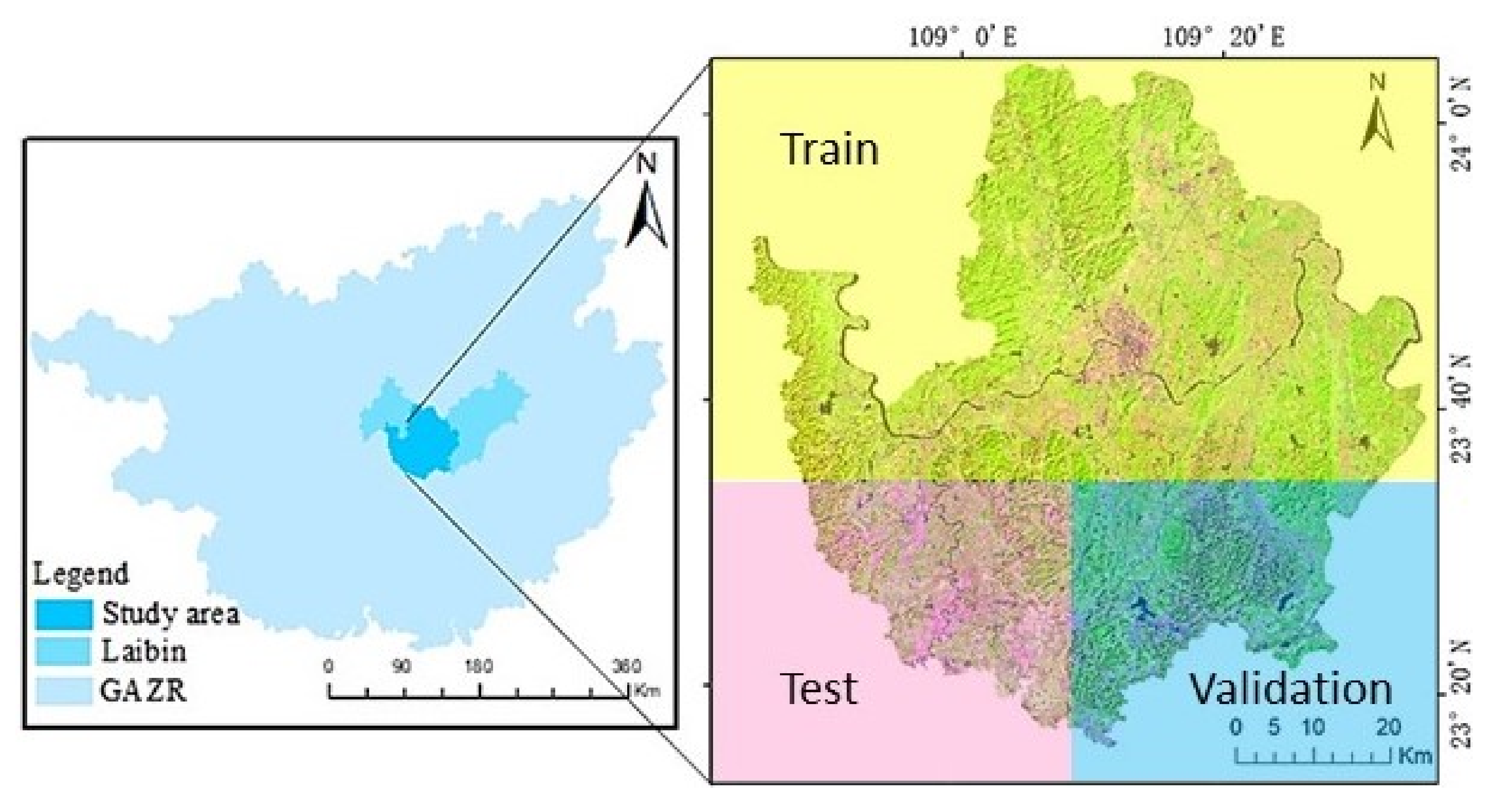
2.1. Study Area Overview

The study area selected for this study is located in Xingbin District, Laibin City, Guangxi Zhuang Autonomous Region (GZAR) (108;43;43E–109;36;07E and 23;15;58N– 24;4;38N) (Figure 1). The study area has a subtropical monsoon climate. The unique climatic and geographical factors make sugarcane one of the major crops in Guangxi, and its planting area accounts for approximately 60% of the country. The planting area of sugarcane in the study area is more than 80% of the total agricultural land, so it is important to accurately and effectively obtain the planting area of sugarcane for local agricultural development, accurate management, and yield estimation.

2.2. Field Sampling and Remote Sensing Image Preprocessing

To obtain the distribution of actual feature types in the study area, a total of 2876 sample points of different feature types were obtained through field data collection and field observations (Table 1). Among sample points, in the process of the field collection of sugarcane and rice samples, priority was given to continuous planting areas with an area larger than 900 m 2 . The acquired data were used to accumulate a priori knowledge and to verify the accuracy at a later stage. In this study, multispectral images covering the study area taken by the Landsat 8 satellite with a resolution of 30 m from 2–8 October 2019, containing 11 bands, were used as the data source (Figure 1). The images from 2–8 October 2019, were taken during the peak growth period of sugarcane and rice. To obtain more effective image information, preprocessing such as geolocation, radiometric calibration, atmospheric correction, mosaicking, and cropping was performed on the images to obtain the sample library data through a combination of indoor supervised classification and field validation, and the sample library data had 4,874,817 samples, 60% of which were used for training, with 20% for validation and 20% for testing (Figure 1). In this paper, high-resolution Sentinel-2 satellite data were used as an aid to validate classification accuracy. The Sentinel-2 Level-C image on 3 October 2019, was downloaded from the USGS website, and the Sentinel-2 Level-C image multispectral data were first corrected for atmosphere, topography, and cirrus clouds using the Sen2Cor software. Subsequently, the SNAP software was used to upsample the bands, increase the resolution to 10 m, and convert them to ENVI format. The 12 bands of the multispectral image were then fused using the ENVI software, and the Seamless Mosaic tool was used to mosaic the image and import the vector data of the study area for cropping. Finally, the latitude and longitude information of the field collected data was imported into the corresponding Sentinel-2 images of the study area to obtain the sample data of the corresponding location, and the classification result map based on the Sentinel-2 images was obtained by supervised classification and accuracy verification of the sample data.

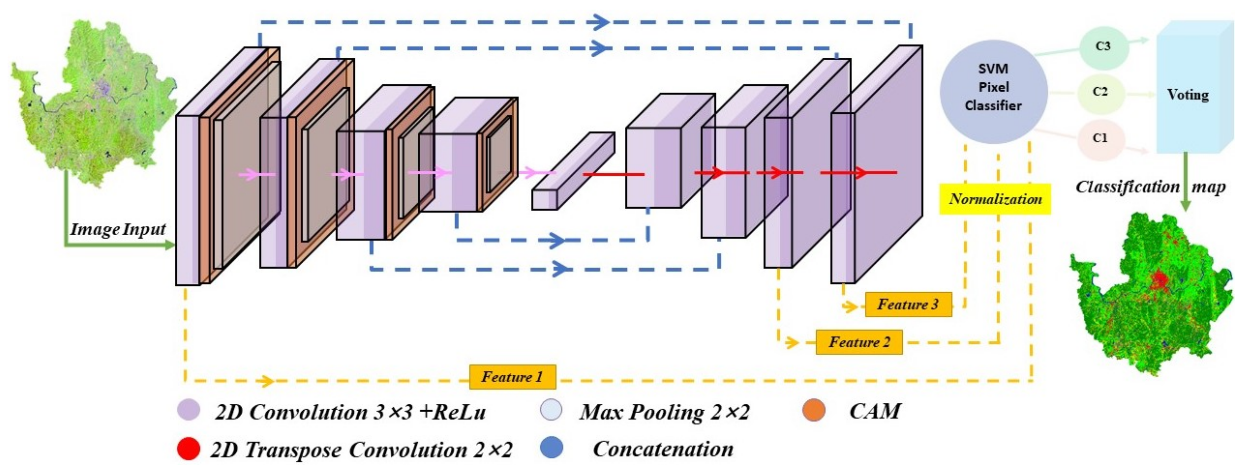
2.3. Improvements to U-Net

As a network goes further, semantic information becomes richer, but spatial resolution becomes lower. To maintain the spatial resolution and semantic features, the U-Net [27] model uses the skip connection operation to fuse the feature maps of different levels. In this paper, we added a channel attention mechanism based on U-Net, used the model trained by the CAM-UNet network to extract three different levels of features, put them into SVM classification, and then analyzed the voting results after the majority voting game to obtain the final results and evaluate classification accuracy. A flowchart of the proposed multifeature fusion perception algorithm framework is shown in Figure 2. The framework consists of four main components: the U-Net model, CAM, SVM classifier, and majority voting game module.

2.3.1. U-Net Model

The U-Net model is an end-to-end semantic segmentation network, which is named U-Net because its structure is symmetrical like the letter U. The U-Net model consists of an input layer, a convolutional layer, a pooling layer, a transposed convolutional layer, an activation function, and an output layer. The convolution layer uses multiple convolution kernels with a size of 3 × 3 and a step size of 1 to perform the convolution operation, and the output after this operation is a feature map. In the convolution process, all input information shares a set of weights (weight sharing), which significantly reduces the training parameters and increases the computational speed. Convolution also has the ability of local perception, which improves neural network signal transmission to a certain extent. The activation operation is the process of increasing the nonlinearization of neural network, which makes the neural network better fit the nonlinear mapping and improves the expressiveness of the model. The commonly used activation functions include sigmoid, Tanh, and ReLU. The U-Net model chooses ReLU as its activation function, which is defined as
R e L U = x x 0 0 x < 0
ReLU has a one-sided suppression capability, outputting directly positive values for positive numbers and zero for numbers less than zero. This capability speeds up network training while converting dense features into sparse features, effectively improving the robustness of the features, and the sparse features are mapped into a high-dimensional feature space with stronger linear differentiability. The essence of transposed convolution is upsampling, and the feature map size is restored to the original image size by multiple transposed convolution operations. The U-Net model proposes the skip connection to retain the information at each level and improve the generalization ability of the network. Upsampling is fused with the downsampled feature channel dimension splicing at the same time, which effectively fuses the image detail information with the contour information. Fusion is performed. Finally, the feature vectors are mapped to the desired number of classes using a 1 × 1 convolution kernel. The loss function, also known as the optimization performance metric, is the optimal performance metric to be achieved by varying the weights of the neural network, and is used to indicate how similar the predicted value is to the true value. U-Net uses boundary weights as its loss function. It is defined as
E = X Ω ω ( x ) log p ( x ) x
where p ( x ) is the loss function of Softmax, and : Ω 1 , , k is the label value of the pixel point.

2.3.2. Classifier

The logistic regression layer of the traditional U-Net model uses the Softmax function to achieve classification, which is based on the principle of regression, and its loss function is a probabilistic model considering global data. It normalizes the data in the feature space and presents the classification results in the form of probabilities. It is defined as follows: Let there be N classes of sample data. The output of the final convolution layer is Y = y 1 , y 2 , , y N T ,and the output after Softmax calculation is S = s 1 , s 2 , , s N T , where
S j = exp y j j = 1 N exp y j
SVM has superior performance compared to Softmax. The basic idea of an SVM is the introduction of a kernel function, which maps linearly indistinguishable features to a high-dimensional feature space and thus makes the feature data linearly distinguishable. The essence of SVM makes the search for the optimal classification hyperplane and does not cause the change in the hyperplane due to the change in nonsupport vector samples. However, in Softmax, any changes in the samples lead to a change in the decision plane.

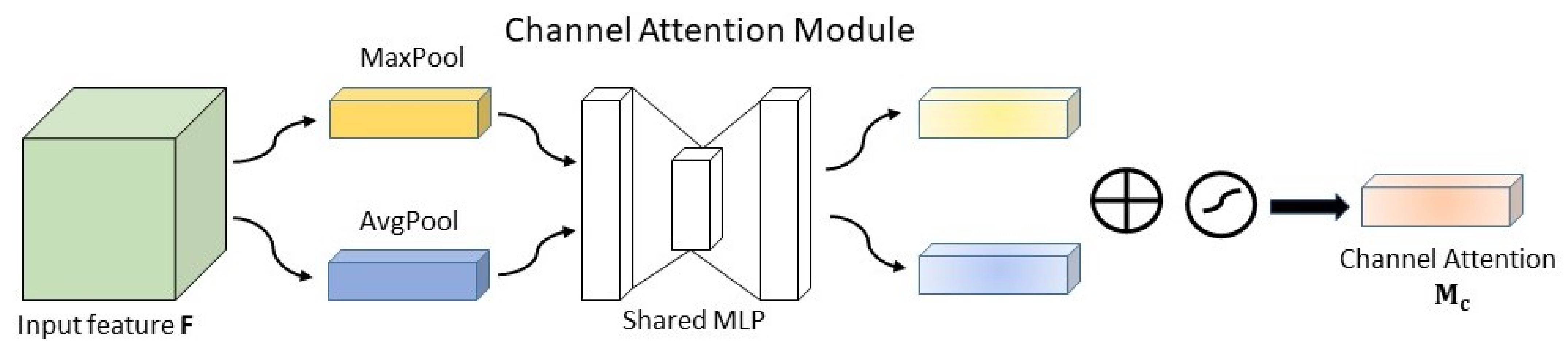
2.3.3. Channel Attention Module

In recent years, the channel attention mechanism has been used for image classification and segmentation with significant success, and it has obtained good results in the field of remote sensing image segmentation [43]. To obtain a more effective feature map, channel attention is introduced to extract image features adaptively before the maximum pooling layer. The specific operation of the CAM is as follows: A feature map (H × W × C) is obtained by global average pooling F a v g c (1 × 1 × C) and global maximum pooling F m a x c (1 × 1 × C). F a v g c and F m a x c are then fed into the shared network consisting of two fully connected layers and an activation layer. Finally F a v g c and F m a x c passing through the shared network are operated by the Add function and fed into the sigmoid function to obtain the channel attention map M c R 1 × 1 × C . Afterwards, the size of the first fully connected layer is R 1 × 1 × C / r , and the size of the second fully connected layer is restored to R 1 × 1 × C . The channel attention module is shown in Figure 3. Channel attention is calculated as follows:

2.3.4. Feature Extraction and Fusion

The most meaningful three levels of the features of the original image are extracted by the network model and put into the SVM for classification, and the final classification is obtained by voting on the three classification results. In this study, to prefer features at different levels, we first extracted images with a size of 256 × 256 containing all classification labels from remote sensing images as experimental samples, and selected all convolutional layers in the network model to train the SVM on the features extracted from the samples separately. The size of the training, validation, and testing samples were 60%, 20%, and 20% of the total sample size, respectively. The features extracted from Layers 2, 56, and 57 of the network model were finally selected for SVM classification through empirical comparison, and the classification results were then subjected to voting games.

2.4. Experimental Environment

In deep learning networks, hyperparameters need to be obtained based on empirical debugging, including the learning rate, the small batch extracted in each iteration, gradient clipping, and other hyperparameters. The learning rate is a hyperparameter that controls the convergence speed of the model. The lower the learning rate is, the slower the change rate of the loss function is and the slower the convergence time is, but it can ensure that the best accuracy is achieved locally. On the contrary, if the learning rate is too high, the local minima will be missed, and the gradient threshold is usually set to enable gradient clipping and suppress the network gradient explosion caused by a very high learning rate. After several experimental debuggings, the experimental learning rate is set to 0.01, and each minibatch contains pixel patches with a size of 256 × 256. There are 30 rounds in total, and 1000 minibatches are extracted in each iteration of each round for a total of 30,000 iterations. The gradient threshold and gradient decay rate are 0.05 and 0.0001, respectively. The code of the experiment is performed using Matlab 2021b, and the experimental environment consists of Intel(R) Core(TM) i5-8500 CPU with an NVIDIA GeForce RTX 2060 GPU.

3. Results

Information on the data categories of the sample pool in the study area is shown in Table 2. Sixty percent was used for training, with 20% for validation and 20% for testing. The following experiments were conducted using the sample pool data in Table 2.

3.1. Model Building

3.1.1. Parameter Optimization and Network Optimization

To verify the effect of MinibatchSize on the network, it was designed with parameter optimization, and overall accuracy (OA), average accuracy (AA), and kappa coefficient were used as evaluation indexes of classification performance. The specific experimental results are shown in Table 3. MinibatchSize is the size of the small batch processing for each training iteration. The larger the MinibatchSize is, the longer it takes for each iteration, but within a certain reasonable range, the larger the MinibatchSize is, the more accurate its determined descent direction is. When MinibatchSize = 8, each iteration takes 1 s, and when MinibatchSize = 16, each iteration takes 2 s. Although it takes twice as long, the overall accuracies of the test set and the real set is improved by 1.66% and 0.5%, respectively, as seen from the comparison of the classification accuracy of U-Net. The accuracies of forestland in the test set and real set were improved by 0.87% and 0.23%, respectively. Because this experiment is for the fine classification of crops, it is worth spending twice as much time to train and improve accuracy.
To verify the effect of different network structures on classification accuracy, this paper compared the U-Net structure with only the channel attention mechanism added (CAM-UNet) with the U-Net structure with both the residual units and attention mechanism added (Res-CAM-UNet) for experimental analysis, and the corresponding experimental results are shown in Table 4. Table 4 shows the effect of residual units on CAM-UNet. Res-CAM-UNet has a higher classification accuracy in sugarcane and construction land compared to CAM-UNet, with an improvement in the test and validation sets: 6.53%, 10.74%, 2.18%, and 5.86%, respectively. However, the classification accuracies obtained in forestland and rice were lower and decreased in the test and validation sets: 30.48%, 41.18%, 3.73%, and 6.71%, respectively.

3.1.2. Comparison of Multiple Methods

To evaluate the performance of deep network methods with multifeature fusion perception in remote sensing classification, the improved algorithm proposed in this paper was compared with U-Net [26], SegNet [25], Attention-UNet [38], SAR-UNet [40], Res-Net [41], Deeplabv3 + ResNet50, Deeplabv3 + Xception and Deeplabv3 + MobileNet [31], the methods were tested and analyzed for comparison. Table 5 and Table 6 show the classification accuracies of the different methods for the test set and validation set of the remote sensing images of the study area. The algorithms proposed in this paper had the highest values of OA, AA, and kappa compared to the other algorithms. In the test set, the OA was also improved by 1.16% after adding an SVM to U-Net, which improved the classification accuracies of forestland, rice, and water bodies. Compared with the original U-Net, the algorithm proposed in this paper improved in each category, and the improvement was greater for rice, water bodies, construction land, forestland, bare land, and other cultivated land: 14.2%, 1.38%, 1.75%, 1.5%, 1.22%, and 5.93%, respectively. The OA was improved by 2.32%. When compared with U-Net + SVM, the OA of the algorithm proposed in this paper was improved by 1.16%, the classification accuracy of each category was slightly improved, and the improvement is more obvious in sugarcane and other cultivated land: 2.41% and 3.17%, respectively. The overall classification accuracy of Deeplabv3+, SegNet, and SAR-UNet was poor. The classification accuracy of SAR-UNet for sugarcane and construction land was the highest. The classification accuracy of Deeplabv3+ was approximately 92% for forestland and 81% for sugarcane. Res-UNet had a higher classification accuracy for water bodies and forestland than other networks after adding the SVM. In the validation set, CAM-UNet + SVM still performed outstandingly, its classification accuracy was superior to those of other networks, except for sugarcane and construction land, and the overall classification accuracy and kappa value were the highest.
Table 7 and Table 8 show the mixture matrix of the algorithm proposed in this paper, and it can be seen that the percentages of forestland, sugarcane, and rice misclassified into each other were large. The probabilities of the misclassification of forestland and rice into sugarcane in the test set were 3.12% and 1.02%. The probabilities of the misclassification of forestland and sugarcane into rice were 18.24% and 2.19%. The probabilities of the misclassification of sugarcane and rice into forestland were 1.39% and 0.71%. The probabilities of the misclassification of forestland and rice as sugarcane in the validation set were 5.71% and 1.41%. The probability of the misclassification of forestland and sugarcane into rice were 16.71% and 3.86%. The probabilities of the misclassification of sugarcane and rice into forestland were 1.08% and 0.88%. Sugarcane, rice, and forestland are misallocated from each other because sugarcane is the most planted cash crop in the study area, covering most of the planting area in the study area, and woodland covers almost half of the study area. The unique spatial distribution resulted in the intersection of the woodland, rice, and sugarcane planting areas. Restricted by the 30 m resolution of the Landsat 8 remote sensing images, the scattered woodlands were not easily distinguished from the rice and sugarcane plantation areas. This also caused the mixing of agricultural land and forestland. The construction land contains cities, villages, and roads. Many rural roads are made of different materials, including stone, dirt, cement, and asphalt. The difference in materials causes some rural roads to be classified as bare land. Villages are surrounded by cropland and woodland, and it is normal that one image element at 30 m resolution may contain construction land, woodland, and cropland and does not distinguish them well.
Figure 4 shows the results of the remote sensing image segmentation of the study area by different methods. As shown in Figure 4, most of the construction land in the study area is concentrated in the central part, and small towns and villages are scattered. The study area is mainly dominated by forests and sugarcane, with few other crops, more concentrated rice cultivation land, and a very low percentage of bare land. In this paper, the decoded data of the Sentinel-2A satellite covering the study area with higher resolution were used to verify the accuracy of the classification results of Landsat 8, and the classification categories and total accuracy of both were roughly the same from the county scale.

3.2. Land Use Change in Laibin

In this study, the 2 November 2010, 14 April 2015, and 2 October 2019 Landsat series images were downloaded from the USGS website (https://earthexplorer.usgs.gov/, accessed on 8 February 2022) to carry out feature classification of the study area, where the 2010 images were Landsat 7 images and the 2015 and 2019 images were Landsat 8 images. To obtain more effective image information, the images were preprocessed with geolocation, radiometric calibration, atmospheric correction, mosaicking, and cropping. Owing to the sensor failure of the Landsat 7 satellite on 31 May 2003, the Landsat 7 images since then have the problem of strip loss, and after its repair, six bands were finally obtained. In this study, higher resolution images and field collection data were used for supervised classification to obtain the sample library data of the 2010 and 2015 study areas, and the algorithm proposed in this paper was used to classify and evaluate the images of the 2010, 2015, and 2019 study areas. Table 9, Table 10 and Table 11 show the mixing matrices of the remote sensing images of the study area in 2010, 2015, and 2019 based on the algorithm proposed in this paper, respectively, and the OAs were 94.02%, 90.41%, and 93.62%, respectively, which meet the needs of the study.
The spatial distribution of land use and land use change are shown in Figure 5. From the spatial distribution of land use, forestland, and sugarcane are the main land use types in the study area, followed by construction land, which is mainly concentrated in the central part, and the rest is scattered in the study area. The main rivers run through the whole study area, and the lakes and reservoirs are distributed more evenly. Rice, bare land, and other arable land are located in a small area. In terms of land use change, there is more conversion of sugarcane to forestland and more conversion of other arable land to forestland and sugarcane.
The types of land use changes in the last decade are shown in Table 12. The area of forestland has the largest ratio to the total area of the study area, followed by sugarcane, other land, construction land, bare land, and rice, and water bodies have the smallest share of the total area of the study area. In terms of land use changes, the areas of forestland, rice, and other cultivated land increased by 25.74%, 116.15%, and 255.37%, respectively. By contrast, the areas of sugarcane, construction land, water bodies, and bare land decreased by 20.15%, 30.13%, 16.16%, and 50.17%, respectively.

3.3. Changes in Forest Dynamics

From the classification results of the remote sensing images of the study area for the three periods of 2010, 2015, and 2019, it can be seen that the algorithm proposed in this paper has the highest classification accuracy for forestland. Therefore, the algorithm was used to monitor the dynamic change of forest resources in the past 10 years, and the forest areas for the three periods in the study area were analyzed and compared. The classification results and dynamic change of forests are shown in Figure 6, and the forest change monitoring area statistics are shown in Table 12. From the results of the forest change monitoring in the study area, it was obtained that the forest area was 1580.59608 km 2 in 2010, 2126.9628 km 2 in 2015, and 1987.4358 km 2 in 2019. The forest area in 2010–2015 increased by 34.56%, whereas the forest area in 2015–2019 decreased by 6.55%. The forest area in 2010–2019 increased by 25.74%. The main reason for the change in forest area is the natural environment and human activities. In 2010–2015, under the call of the Chinese government’s policy of returning farmland to forest, people planted trees to make the overall forest area increase significantly. The forest area in 2015–2019 decreased overall, mainly because eucalyptus trees planted under the policy of returning farmland to forest absorbed a high amount of groundwater, which caused drought in some areas. Therefore, the government introduced a new policy to encourage farmers to plant trees that benefit the ecological environment more than eucalyptus trees, so it is normal for some of the area to decrease and for some forestland to be converted into cropland.

4. Discussion

The traditional U-Net fuses multilayer features while upsampling, and the fused features are then trained. On the other hand, multifeature fusion adds the channel attention mechanism to U-Net, fuses the multilayer features into the network model, extracts the optimal three levels of features for SVM classification, and performs the majority voting game on the three classification results. The algorithm adopts the form of multifeature cascade to reduce the problem of gradient dispersion, and introduces channel attention to assign feature weights, which is a big improvement compared with U-Net. Remote sensing image classification has many difficulties from the acquisition of remote sensing image resources to classification, and the sample size has a great influence on the results. As shown in Table 5, the U-Net segmentation accuracy is higher than that of Deeplabve3+ and SegNet, which are basic semantic segmentation models, so U-Net is chosen as the backbone network. The features obtained by SAR-UNet after the SE module are combined with the upsampled features so that it can have good results for the objects with very obvious single features such as sugarcane, cities and water bodies, which are more beneficial for the binary classification problem. In this paper, the feature map obtained by CAM-UNet was only connected to the pooling layer without combining with the upsampled features, which made the attention domain larger and more beneficial for the multiclassification of remote sensing images. By combining with jump links, there was no significant improvement in the classification accuracy of the multispectral remote sensing images in the study area compared with U-Net, which may be more suitable for super-resolution remote sensing images. The OA was improved after adding U-Net network to SVM. Thus, extracting different levels of feature classification and then performing the majority voting game reduced misclassification to a certain extent. The accuracy of woodland and sugarcane planting area in this study was relatively satisfactory, but misclassifying woodland into sugarcane planting area was larger, as observed by the data sampled in the field. Woodland will be mixed in the large area of sugarcane and rice planting area, and sugarcane and rice will be planted around the large area of woodland. Further extraction of the planting areas of woodland, sugarcane and rice on Landsat 8 remote sensing images is the direction that needs further research.

5. Conclusions

U-Net suffers from insufficient information utilization and pays insufficient attention to some features. In this study, to improve and optimize the U-Net, we combined it with a CAM and replaced the classifier of the original U-Net with an SVM. The CAM-UNet model was used to extract multiple features from the study area, and the SVM, in turn, was used to classify multiple features. The final classification results were obtained using the majority voting game on the classification results of each feature, and the accuracy of the classification results was evaluated and analyzed with the field research data. We used a multifeature cascade to reduce gradient divergence and added a CAM to each convolutional unit of the U-Net encoder to make the network learn image features adaptively and focus more on important features. The results showed that the improved deep network algorithm with multifeature fusion perception has better classification results with images in the study area compared to U-Net, SegNet, Deeplabv3+, Attention-UNet, SAR-UNet, and Res-UNet. Adding the channel attention mechanism to the U-Net encoder can effectively improve network performance, and using the classification results of SVM for the majority voting game can reduce misclassification and improve classification accuracy, especially in forestland monitoring. This improved depth network algorithm based on multifeature fusion perception can better identify feature information and can effectively improve the classification accuracy of remote sensing images. This algorithm can provide a new technical reference for remote sensing image classification.

Author Contributions

Conceptualization, C.Y. and X.F.; methodology, C.Y. and X.F.; software, C.Y. and X.F.; validation, C.Y.; formal analysis, C.Y. and X.F.; investigation, C.Y. and X.F.; resources, X.F.; data curation, C.Y.; writing—original draft preparation, C.Y.; writing—review and editing, C.Y., X.F., J.F. and N.W. All authors have read and agreed to the published version of the manuscript.

Funding

This research was supported in part by the National Natural Science Foundation of China under Grant 62001129, in part by the Guangxi Natural Science Foundation under Grant 2021GXNSFBA075029, and in part by the Guangxi Science and Technology Base and Talent under Project AD19245130.

Data Availability Statement

The code and models are publicly available at https://github.com/Yancccccc/CAM-UNet-SVM, accessed on 8 February 2022.

Conflicts of Interest

The authors declare no conflict of interest.

Abbreviations

Abbreviation Full name
BPBack propagation
SVMSupport vector machine
CNNDeep convolutional neural network
ELMExtreme learning machine
FCNFully convolution network
CRFConditional Random Fields
ASPPAtrous spatial pyramid pooling
SESqueeze and Excitation
CAMChannel attention moudle
GZARGuangxi Zhuang Autonomous Region

References

  1. Lu, B.; Dao, P.D.; Liu, J.; He, Y.; Shang, J. Recent Advances of Hyperspectral Imaging Technology and Applications in Agriculture. Remote Sens. 2020, 12, 2659. [Google Scholar] [CrossRef]
  2. Cheng, T.; Yang, Z.; Inoue, Y.; Zhu, Y.; Cao, W. Preface: Recent Advances in Remote Sensing for Crop Growth Monitoring. Remote Sens. 2016, 8, 116. [Google Scholar] [CrossRef] [Green Version]
  3. Sishodia, R.P.; Ray, R.L.; Singh, S.K. Applications of Remote Sensing in Precision Agriculture: A Review. Remote Sens. 2020, 12, 3136. [Google Scholar] [CrossRef]
  4. Zhao, P.; Wang, D.; He, S.; Lan, H.; Chen, W.; Qi, Y. Driving forces of NPP change in debris flow prone area: A case study of a typical region in SW China. Ecol. Indic. 2020, 119, 106811. [Google Scholar] [CrossRef]
  5. Lv, Z.; Liu, T.; Shi, C.; Benediktsson, J.A.; Du, H. Novel Land Cover Change Detection Method Based on k-Means Clustering and Adaptive Majority Voting Using Bitemporal Remote Sensing Images. IEEE Access 2019, 7, 34425–34437. [Google Scholar] [CrossRef]
  6. Wang, J.; Jiang, L.; Wang, Y.; Qi, Q. An Improved Hybrid Segmentation Method for Remote Sensing Images. ISPRS Int. J. Geo-Inf. 2019, 8, 543. [Google Scholar] [CrossRef] [Green Version]
  7. Menon, R.V.; Kalipatnapu, S.; Chakrabarti, I. High speed VLSI architecture for improved region based active contour segmentation technique. Integration 2021, 77, 25–37. [Google Scholar] [CrossRef]
  8. Tianyang, D.; Jian, Z.; Sibin, G.; Ying, S.; Jing, F. Single-Tree Detection in High-Resolution Remote-Sensing Images Based on a Cascade Neural Network. ISPRS Int. J. Geo-Inf. 2018, 7, 367. [Google Scholar] [CrossRef] [Green Version]
  9. Sun, G.; Rong, X.; Zhang, A.; Huang, H.; Rong, J.; Zhang, X. Multi-scale mahalanobis kernel-based support vector machine for classification of high-resolution remote sensing images. Cogn. Comput. 2021, 13, 787–794. [Google Scholar] [CrossRef]
  10. Li, L.; Jing, W.; Wang, H. Extracting the Forest Type From Remote Sensing Images by Random Forest. IEEE Sens. J. 2021, 21, 17447–17454. [Google Scholar]
  11. Li, W.; Wang, Z.; Wang, Y.; Wu, J.; Wang, J.; Jia, Y.; Gui, G. Classification of High-Spatial-Resolution Remote Sensing Scenes Method Using Transfer Learning and Deep Convolutional Neural Network. IEEE J. Sel. Top. Appl. Earth Obs. Remote Sens. 2020, 13, 1986–1995. [Google Scholar] [CrossRef]
  12. Zhang, C.; Gao, S.; Yang, X.; Li, F.; Yue, M.; Han, Y.; Zhao, H.; Zhang, Y.; Fan, K. Convolutional Neural Network-Based Remote Sensing Images Segmentation Method for Extracting Winter Wheat Spatial Distribution. Appl. Sci. 2018, 8, 1981. [Google Scholar] [CrossRef] [Green Version]
  13. Boualleg, Y.; Farah, M.; Farah, I.R. Remote Sensing Scene Classification Using Convolutional Features and Deep Forest Classifier. IEEE Geosci. Remote Sens. Lett. 2019, 16, 1944–1948. [Google Scholar] [CrossRef]
  14. Guo, Y.; Cao, H.; Bai, J.; Bai, Y. High Efficient Deep Feature Extraction and Classification of Spectral-Spatial Hyperspectral Image Using Cross Domain Convolutional Neural Networks. IEEE J. Sel. Top. Appl. Earth Obs. Remote Sens. 2019, 12, 345–356. [Google Scholar] [CrossRef]
  15. Marmanis, D.; Datcu, M.; Esch, T.; Stilla, U. Deep Learning Earth Observation Classification Using ImageNet Pretrained Networks. IEEE Geosci. Remote Sens. Lett. 2016, 13, 105–109. [Google Scholar] [CrossRef] [Green Version]
  16. Kussul, N.; Lavreniuk, M.; Skakun, S.; Shelestov, A. Deep learning classification of land cover and crop types using remote sensing data. IEEE Geosci. Remote Sens. Lett. 2017, 14, 778–782. [Google Scholar] [CrossRef]
  17. Alshehhi, R.; Marpu, P.R.; Woon, W.L.; Mura, M.D. Simultaneous extraction of roads and buildings in remote sensing imagery with convolutional neural networks. ISPRS J. Photogramm. Remote Sens. 2017, 130, 139–149. [Google Scholar] [CrossRef]
  18. Csillik, O.; Cherbini, J.; Johnson, R.; Lyons, A.; Kelly, M. Identification of citrus trees from unmanned aerial vehicle imagery using convolutional neural networks. Drones 2018, 2, 39. [Google Scholar] [CrossRef] [Green Version]
  19. Wang, P.; Zhang, X.; Hao, Y. A method combining CNN and ELM for feature extraction and classification of SAR image. J. Sens. 2019, 2019, 6134610. [Google Scholar] [CrossRef]
  20. Cao, X.; Gao, S.; Chen, L.; Wang, Y. Ship recognition method combined with image segmentation and deep learning feature extraction in video surveillance. Multimed. Tools Appl. 2020, 79, 9177–9192. [Google Scholar] [CrossRef]
  21. Meng, X.; Zhang, S.; Zang, S. Lake wetland classification based on an SVM-CNN composite classifier and high-resolution images using wudalianchi as an example. J. Coast. Res. 2019, 93, 153–162. [Google Scholar] [CrossRef]
  22. Sun, X.; Liu, L.; Li, C.; Yin, J.; Zhao, J.; Si, W. Classification for remote sensing data with improved CNN-SVM method. IEEE Access 2019, 7, 164507–164516. [Google Scholar] [CrossRef]
  23. Shelhamer, E.; Long, J.; Darrell, T. Fully Convolutional Networks for Semantic Segmentation. IEEE Trans. Pattern Anal. Mach. Intell. 2016, 39, 640–651. [Google Scholar] [CrossRef] [PubMed]
  24. Fu, G.; Liu, C.; Zhou, R.; Sun, T.; Zhang, Q. Classification for high resolution remote sensing imagery using a fully convolutional network. Remote Sens. 2017, 9, 498. [Google Scholar] [CrossRef] [Green Version]
  25. Badrinarayanan, V.; Kendall, A.; Cipolla, R. Segnet: A deep convolutional encoder-decoder architecture for image segmentation. IEEE Trans. Pattern Anal. Mach. Intell. 2017, 39, 2481–2495. [Google Scholar] [CrossRef]
  26. Ronneberger, O.; Fischer, P.; Brox, T. U-net: Convolutional networks for biomedical image segmentation. In International Conference on Medical image Computing and Computer-Assisted Intervention; Springer: Berlin/Heidelberg, Germany, 2015; pp. 234–241. [Google Scholar]
  27. Li, H.; Wang, C.; Cui, Y.; Hodgson, M. Mapping salt marsh along coastal South Carolina using U-Net. ISPRS J. Photogramm. Remote Sens. 2021, 179, 121–132. [Google Scholar] [CrossRef]
  28. Xu, Q.; Yuan, X.; Ouyang, C.; Zeng, Y. Attention-Based Pyramid Network for Segmentation and Classification of High-Resolution and Hyperspectral Remote Sensing Images. Remote Sens. 2020, 12, 3501. [Google Scholar] [CrossRef]
  29. Zhang, H.; Liu, M.; Wang, Y.; Shang, J.; Liu, X.; Li, B.; Song, A.; Li, Q. Automated delineation of agricultural field boundaries from Sentinel-2 images using recurrent residual U-Net. Int. J. Appl. Earth Obs. Geoinf. 2021, 105, 102557. [Google Scholar] [CrossRef]
  30. Zeyada, H.H.; Mostafa, M.S.; Ezz, M.M.; Nasr, A.H.; Harb, H.M. Resolving phase unwrapping in interferometric synthetic aperture radar using deep recurrent residual U-Net. Egypt. J. Remote Sens. Space Sci. 2022, 25, 1–10. [Google Scholar] [CrossRef]
  31. Chen, L.C.; Zhu, Y.; Papandreou, G.; Schroff, F.; Adam, H. Encoder-decoder with atrous separable convolution for semantic image segmentation. In Proceedings of the European Conference on Computer Vision (ECCV), Munich, Germany, 8–14 September 2018; pp. 801–818. [Google Scholar]
  32. He, K.; Zhang, X.; Ren, S.; Sun, J. Deep residual learning for image recognition. In Proceedings of the IEEE Conference on Computer Vision and Pattern Recognition, Las Vegas, NV, USA, 27–30 June 2016; pp. 770–778. [Google Scholar]
  33. Szegedy, C.; Ioffe, S.; Vanhoucke, V.; Alemi, A.A. Inception-v4, inception-resnet and the impact of residual connections on learning. In Proceedings of the Thirty-First AAAI Conference on Artificial Intelligence, San Francisco, CA, USA, 4–9 February 2017. [Google Scholar]
  34. Sandler, M.; Howard, A.; Zhu, M.; Zhmoginov, A.; Chen, L.C. Mobilenetv2: Inverted residuals and linear bottlenecks. In Proceedings of the IEEE Conference on Computer Vision and Pattern Recognition, Salt Lake City, UT, USA, 18–22 June 2018; pp. 4510–4520. [Google Scholar]
  35. Chollet, F. Xception: Deep learning with depthwise separable convolutions. In Proceedings of the IEEE Conference on Computer Vision and Pattern Recognition, Honolulu, HI, USA, 21–26 July 2017; pp. 1251–1258. [Google Scholar]
  36. Woo, S.; Park, J.; Lee, J.Y.; Kweon, I.S. Cbam: Convolutional block attention module. In Proceedings of the European Conference on Computer Vision (ECCV), Munich, Germany, 8–14 September 2018; pp. 3–19. [Google Scholar]
  37. Ge, Z.; Cao, G.; Shi, H.; Zhang, Y.; Li, X.; Fu, P. Compound Multiscale Weak Dense Network with Hybrid Attention for Hyperspectral Image Classification. Remote Sens. 2021, 13, 3305. [Google Scholar] [CrossRef]
  38. Oktay, O.; Schlemper, J.; Folgoc, L.L.; Lee, M.; Heinrich, M.; Misawa, K.; Mori, K.; McDonagh, S.; Hammerla, N.Y.; Kainz, B.; et al. Attention u-net: Learning where to look for the pancreas. arXiv 2018, arXiv:1804.03999. [Google Scholar]
  39. Pham, V.T.; Tran, T.T.; Wang, P.C.; Chen, P.Y.; Lo, M.T. EAR-UNet: A deep learning-based approach for segmentation of tympanic membranes from otoscopic images. Artif. Intell. Med. 2021, 115, 102065. [Google Scholar] [CrossRef] [PubMed]
  40. Wang, J.; Lv, P.; Wang, H.; Shi, C. SAR-U-Net: Squeeze-and-excitation block and atrous spatial pyramid pooling based residual U-Net for automatic liver CT segmentation. arXiv 2021, arXiv:2103.06419. [Google Scholar] [CrossRef] [PubMed]
  41. Cao, K.; Zhang, X. An improved res-unet model for tree species classification using airborne high-resolution images. Remote Sens. 2020, 12, 1128. [Google Scholar] [CrossRef] [Green Version]
  42. Tan, M.; Le, Q. Efficientnet: Rethinking model scaling for convolutional neural networks. In Proceedings of the International Conference on Machine Learning, PMLR, Long Beach, CA, USA, 9–15 June 2019; pp. 6105–6114. [Google Scholar]
  43. John, D.; Zhang, C. An attention-based U-Net for detecting deforestation within satellite sensor imagery. Int. J. Appl. Earth Obs. Geoinf. 2022, 107, 102685. [Google Scholar] [CrossRef]
Figure 1. Location of the study area and Landsat 8 remote sensing images.
Remotesensing 14 01118 g001
Figure 2. Algorithm network framework.
Remotesensing 14 01118 g002
Figure 3. Channel attention module.
Remotesensing 14 01118 g003
Figure 4. Comparison of remote sensing image classification results of the study area by different methods, where (al) are, in order, the ground truth category, Sentinel-2A, CAM-UNet+SVM, U-Net, SegNet, Attention-UNet, SAR-UNet, UNet+SVM, Res-UNet+SVM, Deeplabve3+Resnet50, Deeplabve3+Xception, and Deeplabve3+MobileNet.
Remotesensing 14 01118 g004
Figure 5. Spatial and temporal distribution of land use in 2010 (a); 2015 (b); 2019 (c); Land use change in 2010–2015 (d); 2015–2019 (e); 2010–2019 (f).
Remotesensing 14 01118 g005
Figure 6. Distribution of forestland in 2010 (a); 2015 (b); 2019 (c); dynamics of forestland in 2010–2015 (d); 2015–2019 (e); 2010–2019 (f).
Remotesensing 14 01118 g006
Table 1. Number of field collections of different sample types.
ClassSugarcaneRiceWaterConstruction
Land
ForestBare LandOther
Land
Total
Samples8263421166656801141332876
Table 2. Category information of the data in the sample pool of the study area.
No.ClassTrainValTest
1Sugarcane1,090,123150,147223,668
2Rice130,73663,05362,050
3Water74,43712,50314,818
4Construction land228,49633,12848,244
5Forest1,219,936510,557443,841
6Bare land142,49646,79883,573
7Other land172,06973,27670,835
Total3,058,293889,462947,029
Table 3. Classification accuracy (%) for different MinibatchSize values of U-Net.
MinibatchSize = 8MinibatchSize = 16
ClassTestValidationTestValidation
Sugarcane90.2489.2892.6890.04
Rice68.5762.5462.6756.48
Water86.6088.6291.8491.59
Construction land92.2892.5688.9390.50
Forest94.7995.0395.6695.26
Bare land84.5683.6088.6287.65
Other land72.2173.8978.6179.33
OA (%)92.4092.4690.7187.80
AA (%)88.7688.2886.0683.96
kappa0.84120.82700.86430.8343
Table 4. Classification results of CAM-UNet and Res-CAM-UNet in the test set and validation set.
CAM-UNetRes-CAM-UNet
ClassTestValidationTestValidation
Sugarcane91.7487.3598.2798.09
Rice77.9179.1747.4337.99
Water92.3392.4794.3691.59
Construction land89.7289.7291.9095.58
Forest97.1497.4193.4190.70
Bare land88.2887.7890.3889.71
Other land84.1984.0686.6484.09
OA (%)92.4092.4690.7187.80
AA (%)88.7688.2886.0683.96
kappa0.89160.87850.86750.8083
Table 5. Comparison of the classification accuracy of different methods on the test set of remote sensing images in the study area (%).
ClassCAM-UNet
+SVM
U-NetSegNetAttention
-UNet
SAR
-UNet
U-Net
+SVM
Res-UNet
+SVM
Deeplabv3
+Resnet50
Deeplabv3
+Xception
Deeplabv3
+MobileNet
Sugarcane92.992.6993.5293.5598.7690.4988.0681.0580.5182.12
Rice 76.962.713.6369.9529.4475.0870.5139.560.6241.6
Water93.2391.8567.3389.7490.3692.5694.3972.4774.2672.17
Construction
land
90.6988.9480.689.9298.7487.8987.3473.8676.7174.63
Forest97.1695.6679.8294.5675.3697.297.8891.5792.6692.95
Bare land89.8488.6262.789.5585.7488.6189.6259.7662.660.96
Other land84.2478.6155.877.0779.1681.0781.4542.7248.8644.2
OA (%)92.8290.575.2690.680.591.6691.2278.0180.6679.3
AA (%)89.2885.5864.7786.3379.6587.5687.0465.8570.8966.95
Kappa0.89760.86430.65150.86660.73070.88070.87370.67910.72030.6973
Table 6. Comparison of the classification accuracy of different methods for the validation set of remote sensing images in the study area (%).
ClassCAM-UNet
+SVM
U-NetSegNetAttention
-UNet
SAR
-UNet
U-Net
+SVM
Res-UNet
+SVM
Deeplabv3
+Resnet50
Deeplabv3
+Xception
Deeplabv3
+MobileNet
Sugarcane89.4390.0491.9492.0798.3586.6985.976.0674.0476.4
Rice 77.2653.512.6167.725.7769.1156.8535.958.3945.63
Water92.8391.5973.8191.7488.7292.3590.7972.9773.9371.46
Construction
land
91.2490.4982.2192.199.6890.0692.4575.4676.2974.09
Forest97.4795.2680.0794.1573.2696.795.5790.3893.1492.61
Bare land89.3787.6564.2689.1186.787.1388.3360.2862.1562.08
Other land84.5979.3356.0679.3978.5481.0282.1243.8749.4445.95
OA (%)92.8989.6974.4890.3376.4790.9589.5277.8881.3380.1
AA (%)88.8883.9865.8586.6178.7286.1584.5764.9969.6366.89
Kappa0.88560.83430.6110.8470.65520.85390.83090.6390.6940.6726
Table 7. Mixing matrix of the test set based on the algorithm proposed in this paper.
ClassSugarcaneRiceWaterConstruction
Land
ForestBare
Land
Other
Land
Total
Sugarcane207,796136291619619523542614221,949
Rice 227847,717411031722388954,490
Water821613,815218113413614,510
Construction land608723143,75342918106548,586
Forest698911,32117910431,2413551092451,187
Bare land20146118924075,080537184,404
Other land397514211727523076283959,66871,903
Total223,66862,05014,81848,244443,84183,57370,835947,029
User’s Accurcy (%)93.6287.5795.2190.0595.5888.9582.98-
Producer’s Accuray (%)92.976.993.2390.6997.1689.8484.24-
OA (%)92.82
Kappa0.8976
Table 8. Mixing matrix of the validation set based on the algorithm proposed in this paper.
ClassSugarcaneRiceWaterConstruction
Land
ForestBare
Land
Other
Land
Total
Sugarcane 134,272 24537725553914493021147,466
Rice 2112 48,717277344748177157,362
Water417211,606158114718512,246
Construction land5623953,02255102071832,628
Forest857410,5343864497,6242042060519,386
Bare land1000618804441,825353847,294
Other land3623116813111332757228561,98373,080
Total150,14763,05312,50333,128510,55746,79873,276889,462
User’s Accurcy (%)91.0584.9394.7792.6495.8188.4484.82-
Producer’s Accuray (%)89.4377.2692.8391.2497.4789.3784.59-
OA (%)92.89
Kappa0.8856
Table 9. Accuracy evaluation table of classification results in 2010.
ClassSugarcaneRiceWaterConstruction
Land
ForestBare
Land
Other
Land
Total
Sugarcane1,738,97816,978824,85730,12525,44455041,841,894
Rice 7186 81,929749657528712803326101,332
Water121065112,631318324341152187120,664
Construction land16,56610,5575001391,47645515,696705440,456
Forest24,36453029376841,712,16411,89736361,756,212
Bare land19,2721818250415,84510,212495,6675545,323
Other land5397373756030294336249969,36788,925
Total1,811,775116,614124,390445,6491,760,013553,63582,7304,894,806
User’s Accurcy (%)94.4180.8593.3488.8897.4990.8978.01-
Producer’s Accuray (%)95.9870.2690.5587.8497.2889.5383.85-
OA (%)94.02
Kappa0.9157
Table 10. Accuracy evaluation table of classification results in 2015.
ClassSugarcaneRiceWaterConstruction
Land
ForestBare
Land
Other
Land
Total
Sugarcane1,115,51128,890214,17058,44665,75448581,287,631
Rice 7946 83,4770129156552923526102,097
Water8164,38139977125069,104
Construction land10,70920952483412,243287723,16010453,577
Forest45,100224327931842,260,52848,00339552,363,292
Bare land45,5038705129,32223,637473,5506529587,247
Other land34772328217753889598217,40133,873
Total1,228,254127,73967,167464,9822,350,654621,746362794,896,821
User’s Accurcy (%)86.6381.7693.1790.8995.6580.6451.37-
Producer’s Accuray (%)90.8265.3595.8588.6696.1776.1647.96-
OA (%)90.41
Kappa0.85842497
Table 11. Accuracy evaluation table of classification results in 2019.
ClassSugarcaneRiceWaterConstruction
Land
ForestBare
Land
Other
Land
Total
Sugarcane 1,388,389 10,65225829836,382913417,8961,470,776
Rice 9091 186,7891321916,838544930219,032
Water52111797,608117654120653101,167
Construction land5289281071286,8891894904960307,745
Forest37,61751,684929212,111,32790357812,208,262
Bare land639422117805139243,45413,905271,730
Other land171065493793567090899812268,055316,018
Total1,463,938255,785101,758309,8682,174,334272,867316,1804,894,730
User’s Accurcy (%)94.4085.2896.4893.2295.6189.5984.82-
Producer’s Accuray (%)94.8473.0395.9292.5897.1089.2284.78-
OA (%)93.62
Kappa0.908313744
Table 12. Changes in land use types in different periods in Xingbin District, Laibin City, 2010–2019.
Class2010
(km 2 )
2015
(km 2 )
2019
(km 2 )
2010–2015
Area Change Rate
2015–2019
Area Change Rate
2010–2019
Area Change Rate
Forest 1580.59 2126.961987.430.3456−0.06560.2574
Sugarcane 1657.7 1158.861323.69−0.30090.1422−0.2015
Construction land396.41408.21276.970.0297−0.3215−0.3013
Rice91.1991.88197.120.00751.14531.1615
Water108.5962.1991.05−0.42730.4639−0.1616
Bare land490.79528.52244.560.0768−0.5373−0.5017
Other land80.0330.48284.41−0.61918.32952.5537
Publisher’s Note: MDPI stays neutral with regard to jurisdictional claims in published maps and institutional affiliations.

