Abstract
The recently proposed multi-objective clustering methods convert the segmentation problem to a multi-objective optimization problem by extracting multiple features from an image to be segmented as clustering data. However, most of these methods fail to consider the impacts of different features on segmentation results when calculating the similarity using the Euclidean distance. In this paper, feature domination is defined to segment the image efficiently, and then an adaptive feature weights based double-layer multi-objective method (AFWDLMO) for image segmentation is presented. The proposed method mainly contains two layers: a weight determination layer and a clustering layer. In the weight determination layer, AFWDLMO adaptively identifies the dominant feature of an image to be segmented and specifies its optimal weight through differential evolution. In the clustering layer, multi-objective clustering functions are established and optimized based on the acquired optimal weight, and a set of solutions with high segmentation accuracy is found. The segmentation results on several texture images and SAR images show that the proposed method is better than several existing state-of-the-art segmentation algorithms.
1. Introduction
Synthetic aperture radar (SAR) is widely applied to many practical applications, such as environmental surveillance, natural disaster monitoring, land resources management, and target detection, which is an advanced active coherent microwave imaging mechanism to produce high-precision images and allows all-day and all-weather acquisitions [1,2]. These applications involve extraction, recognition, understanding, and analysis of SAR images in the field of computer vision. SAR image segmentation, considered to be more difficult than natural image segmentation, is a fundamental step in image interpretation and scene understanding. The process is to divide an SAR image into several non-overlapping regions by the different structural properties such that the difference between pixels in the same region is small, while, in different regions, it is large. Among the exiting segmentation approaches such as partial differential equation-based segmentation, threshold methods, edge-based segmentation, region-based segmentation, deep-learning-based segmentation, and so on, clustering-based segmentation is a popular one and has attracted more and more attention in recent years [3].
The fuzzy theory is incorporated into clustering algorithms to retain as much information from the original image as possible. As a classical method, fuzzy c-means (FCM) [4] has been widely used in various applications [5,6,7,8]. FCM constantly updates the clustering center and membership matrix until it satisfies the terminating condition (maximum iteration or the difference of objective function between adjacent generations is less than a certain value), and satisfactory solutions are obtained at the end. Based on these solutions, the cluster label of each segmentation unit is determined, and then a segmentation map of the original image can be generated. However, FCM and its variants are usually sensitive to the initialization and easily trapped into the local optimum. To overcome this limitation, many works have been done by researchers at home and abroad to modify FCM [9,10,11,12,13,14].
The clustering methods based on evolutionary algorithms (EAs) alleviate the sensitivity to the initialization and can easily jump out of the local optimal region with its powerful global search capability. In the previous studies, various single-objective clustering algorithms based on EA have been proposed [15,16,17,18,19,20,21,22]. However, a single objective cannot adequately and accurately represent the structures of complex SAR images. Moreover, the single-objective clustering algorithms are also generally trapped into local optimal, making it difficult to obtain optimal segmentation results. Naturally, there is a need for simultaneously optimizing multiple objective functions to explore the different structures from SAR images [23].
Recently, multi-objective clustering methods have gradually replaced single-objective clustering methods as a research hotspot for image segmentation. In [24], the Voronoi initialized evolutionary nearest-neighbor algorithm (VIENNA) is proposed, which optimizes two objective functions based on the Pareto envelope-based selection algorithm (PESA-II) [25]. It utilizes a direct individual encoding that each data point corresponds to an allele, and specifies the cluster to which each data point belongs. However, VIENNA does not provide a strategy to select a suitable solution from the final Pareto front (PF). In [26], the two authors modified VIENNA and presented a multi-objective clustering with an automatic k-determination (MOCK) algorithm, which adopts the minimal spanning tree to encode individuals without specifying the number of clusters and develops a strategy of selecting a satisfactory solution from the Pareto front optimized by PESA-II. In [27], several fuzzy clustering criteria acted as objective functions, are considered to tackle the fuzzy partitioning problem, and are simultaneously optimized in the framework of the fast non-dominated sorting genetic algorithm (NSGA-II) [28]. In [29], Yang et al. applied the immune clone algorithm to SAR image segmentation by optimizing two fuzzy clustering validity indices and constructed the fused feature between the Gabor and GLCM features. In [30], Zhong et al. proposed a two-layer clustering method, including an optimization layer and a clustering layer. In the optimization layer, the optimal number of clusters is determined by minimizing [4]. In the clustering layer, the clustering results can be obtained by optimizing and [31] based on NSGA-II. In [32], Ma et al. presented an adaptive multi-objective memetic clustering algorithm that achieves a balance between the global and local search capabilities through differential evolution (DE) [33] and Gaussian local search adaptively. However, the algorithm is sensitive to noises due to failing to consider spatial and contextual information. In [34], Gao et al. developed a multi-objective fuzzy clustering method that can improve the robustness to noise and outliers by introducing local spatial and grey level information together. In [35], Zhao et al. proposed a multi-objective spatial fuzzy clustering algorithm for SAR image segmentation that constructs fuzzy objective functions with image spatial information to overcome the sensitivity to noises. In [36], Zhang et al. introduced a multi-objective clustering method based on decomposition (MOEA/D) [37] for optimizing the original FCM function and the local information-based function to improve the search capability. In [38], Saha et al. presented a multi-objective DE based fuzzy clustering technique that adopts two mutation operators exchanged by the number of iterations to enhance search capability. In [39], a multi-objective genetic algorithm based on NSGA-II is proposed, which provides promising solutions in well-separated, overlapping clusters from real-life data sets.
Over five years, deep learning has been popular in remote sensing communities. Deep learning methods aim to perform extraction of multi-layer features representation from images, which achieve more accurate results and have been successful in image processing, involving complicated steps and a large number of calculations. Due to the special coherent imaging mechanism, there are speckle noises and overlapped phenomena in SAR images, making the interpretation of SAR images quite difficult. In addition, as typical data-driven methods, deep learning methods are affected due to few free SAR datasets [40] and requiring high-quality annotated data together with demanding specialty-oriented knowledge and skills. Therefore, compared with general optical images, there are few related works on deep learning for SAR images. In [41], Duan et al. proposed an SAR image segmentation method based on convolutional-wavelet neural networks (CWNN) and Markov Random Field (MRF). In a convolutional neural network (CNN), max-pooling does not consider the structure of the previous layer, blindly taking the maximum value in the rectangular window as the output, which may cause the loss of some structures. Wavelet transform [42,43,44,45,46] is a popular mathematical tool for time-frequency analysis and can be used to analyze different proportions of signals [47]. For image processing, the high-frequency proportion represents the edges and textures of images, while the low-frequency proportion represents the smooth part of images. Thus, the wavelet transform is integrated into CNN to enhance the performance in [41]. Furthermore, CWNN was used with two labeling strategies (a superpixel approach and an MRF approach) to produce the final segmentation results. Moreover, in [47], Bi et al. present a contextual PolSAR image semantic segmentation method, which simultaneously utilized three-dimensional discrete wavelet transform features and MRF priors firstly; contextual information is fully integrated during the segmentation to ensure accurate and smooth segmentation. In [48], Xia et al. provide benchmark high-resolution GaoFen-3 SAR datasets, and review the state-of-the-art semantic segmentation methods applied to the construct SAR datasets.
Compared with deep learning methods, multi-objective fuzzy clustering methods capture a good description of fuzzy areas in SAR images [40], involving few calculations. They achieve unsupervised segmentation of complex SAR images, requiring little or no prior knowledge about those images. In addition, they meet the needs of those images with a small scale. Most of the multi-objective clustering methods utilize the Euclidean distance to calculate the similarity between pixels. If only one feature is extracted from an image, the segmentation performance is not affected by the Euclidean distance. Nevertheless, a single feature cannot represent the complicated structures of SAR images. Naturally, multiple features are extracted to achieve a better description of SAR images. In this paper, the concept of feature domination between two features is firstly introduced, and then a combined feature is constructed by two features to segment an image. The dominant feature with higher segmentation accuracy necessarily plays a dominant role in the segmentation, but the Euclidean distance fairly treats each dimension in the combined feature vector. In such a scenario, the dominant feature between features should be identified and adequately utilized to improve the segmentation accuracy. To address the above issues, the adaptive feature weights based double-layer multi-objective method for image segmentation is proposed, which mainly contains two layers: a weight determination layer and a clustering layer. In the weight determination layer, DE is utilized to identify the dominant feature and assign it to an additional weight (called feature weight) by optimizing a corresponding objective function. In the clustering layer, a multi-objective clustering method is implemented to segment an image by optimizing simultaneously two objective functions. These two objective functions are modified by the feature weight.
2. Basic Knowledge
2.1. Multi-Objective Problem (MOP)
In practice, many problems can be modeled as multiple objectives. Objectives often conflict with each other and cannot obtain one optimal solution but a set of solutions that present different trade-offs among objectives [49]. Without loss of generality, a minimization multi-objective optimization problem can be defined as
where is the decision space, x is the n-dimensional decision(variable) vector, and is the M-dimensional objective vector.
For two solutions and , is said to dominate if for each and at least one . A solution is a Pareto optimal solution if there is no other solution dominating . Then, is a Pareto optimal(objective) vector. The set of all Pareto optimal solutions is called Pareto set. Mapping the Pareto set into the objective space results in a set of Pareto optimal objective vectors, called Pareto front [50].
2.2. MOEA/D
A multi-objective clustering problem for image segmentation generally is transformed into an MOP that is resolved by an appropriate method. In this work, MOEA/D is adopted to solve the MOP, which converts an MOP into multiple single-objective subproblems based on a set of weight vectors. There are three decomposition approaches for MOEA/D widely used, including the weighted sum, the Tchebycheff approach, and the penalty-based boundary intersection approach. The weighted sum methods can work well for convex PFs but not for non-convex ones [37]. The Tchebycheff method can overcome this limitation and is expressed as
where is a weight vector in the objective space, and is the reference point, i.e.,
For general multi-objective clustering methods, there is a need for calculating all the objective values to check the dominant relationship between and in the population. Nevertheless, for MOEA/D, the relationship between each pair of individuals can be specified by only comparing two Chebyshev values. Different Pareto optimal solutions can be obtained by adjusting the weight vectors. If the weight vectors are uniformly distributed, the Pareto optimal solutions also tend to be uniformly distributed. Furthermore, the process of MOEA/D to obtain a set of better convergence solutions in detail is as follows. Initialize a set of weight vectors uniformly distributed, bind the vectors to each individual, then optimize continuously the individuals on each weight vector to make them get closer to the Pareto front. In the process, the Chebyshev formula is applied to compare each pair of solutions.
3. Adaptive Feature Weights Based Double-Layer Multi-Objective Method for SAR Image Segmentation
3.1. Motivation
SAR image segmentation is a challenging task due to two main reasons. On the one hand, SAR images have rich characteristic information, such as amplitude, phase, polarization, and so on. On the other hand, there are speckle noises and overlapped phenomena in SAR images. An image can be described by different features that vary in properties, physical meaning, dimension, and performance on segmentation. Consequently, the concept of feature domination is proposed to obtain a better description of an image. Two features and are extracted from an image, where is dominant if achieves higher segmentation accuracy than .
Given the first feature and the second feature , the combined feature is adopted to segment an image. Thus, the total similarity between x and a cluster center is defined as
where the two independent feature similarities and are expressed as
In the combined feature, the effect of one feature on the segmentation mainly includes two factors: (1) feature dominance; (2) dimension of the feature, involving two cases as follows:
Case 1: A feature is dominant in the image, and its dimension is higher.
Case 2: A feature is dominant in the image, but its dimension is lower.
In case 1, let be dominant and . plays a decisive role in Equation (3), indicating that using Euclidean distance makes the proportions of the higher-dimension feature improve. It is naturally concluded that the segmentation accuracy is extremely improved by the dominant feature with higher dimension. However, the dominant feature is inadequately utilized in this case.
In case 2, let be dominant but . plays a decisive role in Equation (3), weakening . It means that using the Euclidean distance reduces the proportion of the lower-dimension feature. Thus, the segmentation accuracy is reduced by the dominant feature with lower dimension.
To overcome the above issues, in the total similarity, a strategy is proposed to raise the proportion of the dominant feature regardless of its dimension. For case 1, if the feature with higher-dimension is dominant, its effects on the total similarity will be further increased by adding a weight greater than 1 to . Accordingly, the effect of the dominant feature can be fully used. For case 2, if the lower-dimension feature is dominant, its proportion in the total similarity will be reduced. There is a need for increasing its weight to make up for the weakened effect by the Euclidean distance. To implement this strategy, there are two aspects involved. On the one hand, the dominant feature is unknown in different images such that the algorithm should identify the dominant feature without prior information. On the other hand, the extra weight assigned to the dominant feature should not be as large as possible, but there is an optimal value that maximizes the segmentation accuracy. Consequently, it is also significant to automatically optimize the additional weight of the dominant feature.
To tackle the above issues, an adaptive feature weights based double-layer multi-objective method for SAR Image segmentation is presented.The proposed framework contains two layers: the weight determination layer and the clustering layer. In the weight determination layer, the main purpose is to identify the dominant feature of the image and determine the optimal weight adaptively, and then transmit the optimal weight to the clustering layer. In the clustering layer, a multi-objective clustering method is used to optimize multiple objectives modified by the optimal weight to capture the segmentation result.
3.2. Feature Extraction
If pixels are directly used as the basic processing unit, there exist two problems in SAR image segmentation. On the one hand, an SAR image is quite large and contains plenty of complex objects, which often need to extract lots of features for representing one pixel. In this way, the process becomes computationally expensive. In addition, there is speckle noise that randomly changes the pixel value in the SAR image, making pixel features unable to accurately represent pixel points and even misleading the algorithm to produce incorrect segmentation. How to suppress the speckle noise is also a matter that should be considered. Instead of pixels, superpixels, which are a set of pixels with certain similarities, are considered as the atomic unit for image processing in this work. The several advantages of using superpixels include: (1) it can reduce the amount of data in the image processing, accelerating the segmentation speed; (2) it can effectively suppress the speckle noise. The average of multiple pixel features is defined as a superpixel feature in this work, which can reduce the influence of outliers to suppress the speckle noise; (3) the extraction methods of superpixels usually utilize spatial information to make the surrounding pixel points fuse into a superpixel. Using spatial information may extremely enhance the segmentation ability, which is exactly what most segmentation methods lack.
Superpixel segmentation aims at grouping pixels in an image into atomic regions whose boundaries align well with the natural object boundaries [51], which is a standard preprocessing step that has been widely used in computer vision and image processing applications [52]. The Watershed segmentation method [53] is applied to divide the image into non-overlapping superpixels in this paper, which is a morphological gradient-based technique. In the original image, different gray values are considered as different heights. The idea is to imagine different heights of the geographical structure, and consider the regional minimum value as the bottom while the surrounding heights are higher than the bottom. Imagine that water flows slowly into the areas, and each sag area is filled with water. When the water between two adjacent concave areas is over the peak, they will fuse, and the connection line will constitute the watershed. All watersheds segment the image into several areas, called superpixels. The watershed segmentation can be described as in Algorithm 1.
In addition, a superpixel feature is computed by the average of all pixel features inside the superpixel, where the gray feature, GLCM feature, Gabor feature, and the combined feature between them can be regarded as the pixel features.
| Algorithm 1 Watershed Segmentation Algorithm |
Input: Image I. Output: Superpixel result. 1 Gradient graph computation: Perform the Sobel filter operation [54] for edge extraction on the input image I to obtain the gradient image; 2 Morphological process: (1) Perform the morphological opening operation on the gradient image; (2) Perform the morphological closing operation on the gradient image; 3 Gradient transformation: Reconstruct the gradient image by the standard watershed transformation. The area inside each watershed is regarded as a superpixel. |
3.3. The Weight Determination Layer
Since DE was first proposed by Storn and Price, DE has been widely used in most optimization fields, such as data mining, pattern recognition, biomedical engineering [55], remote sensing image processing [56], and so on. DE is a global search algorithm based on population and finding the solutions to problems. The encoding method of a standard DE is real number encoding, which makes the algorithm perform well in most complex optimization problems combined with its mutation, crossover, and selection operations [57]. In this section, an improved single-objective optimization model based on DE is used to identify the dominant feature of an image and obtain its optimal weight adaptively. Firstly, the feature weight is encoded into each individual in the initial population. Thereafter, DE is applied to optimize a single objective to obtain the optimal individual. Meanwhile, for the given image, the dominant feature will be correctly found by the optimal weight. The following will present all steps in detail.
3.3.1. Initialization
In the weight determination layer, an individual is encoded as shown in Figure 1. Here, the number of clusters K is set predefined. The top K codes are cluster centers, and the last one is the feature weight.

Figure 1.
Individual encoding of the AFWDLMO algorithm.
The cluster center is randomly selected from the decision space (the whole image), and feature weight w is an integer randomly selected from . If , reselect until .
3.3.2. The Similarity and Membership with Weight
The feature weight w is assigned to the corresponding similarity in Equation (3). If , is dominant and the total similarity is computed by Equation (5). Otherwise, is dominant and the total similarity is computed by Equation (6):
The membership between the data point and the cluster center is defined as Equation (7) if . Otherwise, the formula can be deduced by Equation (6):
where is the Euclidean distance between and , namely the similarity; m denotes the fuzzy coefficient. In this work, m is set to be 2, which is commonly used.
3.3.3. The Objective Function with Weight
A corresponding single objective function for texture images or SAR images is optimized by DE. After a lot of generations, the optimal objective value is obtained, and the w in the optimal individual is the feature weight. Meanwhile, the dominant feature is determined according to the sign of w.
For the texture images, the clustering accuracy to be maximized is defined as
denotes the number of data points that are correctly clustered, and is the total number of data points. The weighted membership between a data point and all cluster centers can be acquired by Equation (7). Each point is put into a cluster center with the greatest membership. In this way, all data points are classified and their labels can be obtained. Eventually, the clustering accuracy of each point is computed by the obtained label and true label.
For SAR images, the objective function is modified by the feature weight. If , is defined as Equation (9); Otherwise, can be deduced by Equation (6):
denotes the compactness of all clusters of the given data set and reflects the within-cluster variance summed. A lower value of indicates a better clustering result.
3.3.4. Evolution
In this section, DE is used to optimize the corresponding objective function. The DE/rand/1 mutation and binomial crossover operations [58] are respectively performed on the parent population to generate the offspring population. A greedy selection by the objective values is utilized to choose individuals for maintaining the population size of the next generation.
3.3.5. The Procedure of the Weight Determination Layer
The procedure of the weight determination layer is described in Algorithm 2.
| Algorithm 2 Weight Determination Layer |
Input: Superpixel result by Algorithm 1, population size N, the number K of clusters, and the parameters of DE. Output: The optimal feature weight w. 1 Initialization: (1) Compute the superpixel features based on the input superpixels; (2) Set ; Generate the initial population by the superpixel features based on the encoding method in Figure 1; (3) For each individual in , calculate the weighted similarity by Equation (5) or 2 Update: (1) Perform the mutation and crossover operations on , and generate the offs- pring population ; (2) For each individual in , calculate the weighted similarity and membership and the corresponding objective value; (3) Implement the selection strategy on and , and generate the next popu- lation ; 3 Stop Criterion: If the termination criterion is satisfied, return to 4; Otherwise, return to 2 and set ; 4 Select the optimal individual from the final population, and then the dominant feature and its optimal weight w can be obtained. |
3.4. The Clustering Layer
In this section, a clustering-based method is adopted to segment the given image. The multi-objective clustering problem is transformed into an MOP firstly, and then the main work is to optimize the MOP based on the MOEA/D. The objectives to be optimized are adapted by the feature weight obtained from the upper layer. After generating a set of Pareto optimal solutions, a satisfactory solution is obtained using a selection strategy.
3.4.1. The Objective Functions with Weight
The weighted and are taken as objective functions that can effectively reflect the image structure to enhance the segmentation performance. In addition, it is demonstrated that and are mutually exclusive in [36], which suits well for multi-objective optimization. is consistent with the weight determination layer as Equation (9). The weighted is expressed as Equation (10) if ; Otherwise, the formula is deduced by Equation (6):
is the ratio of the total variation to the minimum separation of the clusters. Similarly, a lower value of implies a better solution.
3.4.2. Selection
For an MOP, a single solution cannot simultaneously satisfy all objectives due to their mutual exclusivities, but a set of Pareto optimal solutions are usually generated. Most multi-objective optimization algorithms provide users with a series of solutions, which requires users to choose a suitable solution according to their preference. Therefore, it is difficult to select a satisfactory solution from the Pareto optimal solutions without uses’ preferences. In addition, there is no prior information about SAR images. Naturally, index [59] that does not require true clustering information of images is adopted to select the best solution from PF. If , is defined as Equation (11). Otherwise, the formula can be deduced by Equation (6):
Here,
and
where N is the total number of points to be clustered. The actual number of clusters can be obtained by maximizing this index.
3.4.3. The Procedure of Clustering Layer
The procedure of the clustering layer is described in Algorithm 3.
| Algorithm 3 Clustering Layer |
Input: The feature weight w determined by Algorithm 2, the number K of clusters, population size N, the parameters of DE, and the neighborhood size K of each weight vector. Output: The cluster labels and final segmentation image. 1 Initialization: (1) Generate weight vectors , which uniformly distribute in the objec- tive space; Initialize the reference point ; (2) For each weight vector, calculate the Euclidean distance with other vectors and work out the T closest weight vectors as its neighborhood; (3) Set ; Generate the initial population ; (4) For each individual in , calculate the weighted similarity by Equation (5) or 2 Update: (1) Implement mutation and crossover on the neighboring individuals of each indi- vidual in , and generate the offspring population ; (2) For each individual in , calculate the weighted membership, and the objec- tive function values and ; (3) Update the reference point , and neighboring individuals of each individual in by comparing the Chebyshev values. 3 Stop Criterion: If the termination criterion is satisfied, return to 4; Otherwise, return to 2 and set ; 4 Select an individual based on the weighted , and then obtain the cluster labels using a membership matrix. |
4. Experimental Design
In this section, four multi-objective clustering algorithms, AFCMOMA [32], AFCMDE [30], MoMODEFC [38], and FCMNSGA [39] are taken as the comparative algorithms. All the comparative methods achieve unsupervised segmentation of SAR images where there is little or no prior knowledge of those images. Furthermore, they are suitable for those images with a small scale and few calculations. Their characteristics are summarized as follows:
(1) AFCMOMA optimizes two objective functions and based on memetic algorithm, which adaptively balances the capabilities of local search and global search in the optimization.
(2) AFCMDE is an automatic fuzzy clustering method based on DE. It is a two-layer model including an optimization layer and a classification layer to obtain the optimal clustering results for remote sensing imagery. In AFCMDE, the clustering problem converts to an MOP using two objective functions: and .
(3) MoMODEFC optimizes and based on DE using the traditional mutation, crossover, and selection operations. It utilizes two mutation operators exchanged by the number of iterations to enhance search capability.
(4) FCMNSGA adopts FCM clustering method based on NSGA-II for data clustering, optimizing and overlap-separation measure. Compared with several clustering techniques, it has shown to be better for handling separated, compact and overlapped clusters.
Some modifications of comparative algorithms are made for fair comparisons. Firstly, the optimized objectives adopt and in all algorithms. The number of cluster centers is set K in AFCMDE and FCMNSGA. For AFCMDE, the best individual is chosen directly by the index in the optimization layer, and then the obtained individual is used to initialize the population in the classification layer.
Four experiments are designed to demonstrate the effectiveness of the proposed algorithm. In the first experiment, all algorithms are performed on six texture images using the combination feature of the GLCM and Gabor feature, where Gabor is the first feature and GLCM is the second feature. In the second experiment, the proposed algorithm is performed on three texture images with speckle noise to further confirm its ability to segment SAR images. In the third experiment, all algorithms are carried out on eight real SAR images using the combination feature of gray and GLCM feature, where the gray feature is the first feature and the GLCM feature is the second feature. In the last experiment, to verify that the proposed method can adaptively adjust the feature weight to different images, the segmentation results of the obtained optimal weights are compared with that of four fixed weights on three texture images.
In all experiments, features are extracted from images including gray features, GLCM features, and Gabor features. For the GLCM feature, the distance of each pair of pixels is set to 1, four directions of , , , and are used. The sliding window with is used to represent the information for each pixel. After obtaining the gray matrix of each pixel, three statistics of contrast, homogeneity, and energy are extracted in each direction to generate GLCM feature with 12 dimensions. For the Gabor feature, the angles are set to , , , , , and . The wavelengths of the Gabor filter are , , , and , respectively. Therefore, the combination of angles and wavelengths generates Gabor features with 24 dimensions. In each experiment, three of the above features extracted from original images are normalized into first.
For fairness, the same parameters have been applied during the segmentation in all algorithms. The population size is 20. The Mutation and crossover probability are 0.5. The maximum number of iterations is 20. The two functions to be optimized are and in all algorithms.
The special experimental settings are summarized as follows: In AFWDLMO, population size in the weight determination layer is set to 20 and the number of iterations is set to 20; the neighborhood size T is set to 5 in the clustering layer. In AFCMOMA, the local mutation rate is set to , and the standard deviations are , , , and 1, respectively. The probability of initial selection is for each standard deviation. In AFCMDE, the numbers of iterations are set to 10 and 20, respectively, for two layers. Noting that AFCMOMA performs many local searches after the global search, and AFCMDE contains an optimization layer that determines the number of clusters before the classification layer, the number of evaluations of them is more than that of other algorithms. In all experiments, the number of independent runs on each image is 20 for all algorithms.
For the texture images, [60] is adopted to evaluate the performance of segmentation results. is defined as Equation (14):
where U and V are two different partitions of all objects. a-objects in a pair are placed in the same group in U and in the same group in V; b-objects in a pair are placed in the same group in U and in different groups in V; c-objects in a pair are placed in the same group in V and in the different groups in U; d-objects in a pair are placed in different groups in U and in different groups in V.
measures the agreement between two partitions in clustering analysis with different numbers of clusters and indicates the similarity between the obtained label and the true label of the image. The higher value of means the closer to the true label and the better the segmentation result. For SAR images, the performance of each algorithm is judged by manually observing the segmentation results because there are no true cluster labels.
4.1. Results on Texture Images
Six texture images are used to evaluate the performance of the proposed AFWDLMO. The texture structures are selected from the Brodatz texture library for each image ( pixels). Gabor features are dominant in Image1 and Image2, and GLCM features are dominant in Image3 and Image4. For Image5 and Image6, Gabor and GLCM features have similar performances on segmentation results, but Gabor feature is slightly better. The final segmentation results are visually shown in Figure 2, Figure 3, Figure 4, Figure 5, Figure 6 and Figure 7, where (a) is the original texture image and (b–f) are segmentation results of five algorithms. In Table 1, the integer column of AFWDLMO represents the feature weights obtained by the weight determination layer, and the best result in each row is highlighted.
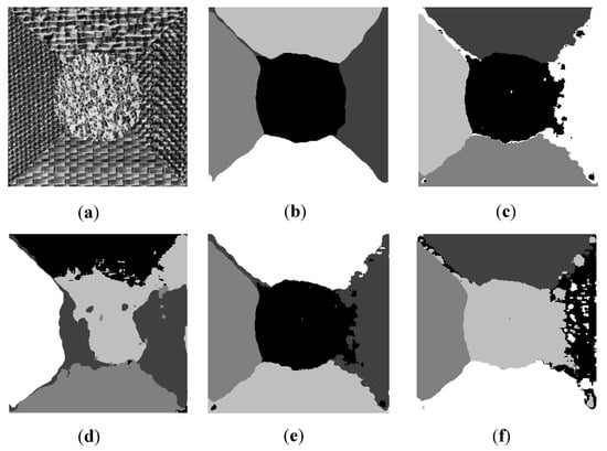
Figure 2.
Segmentation results on Image1. (a) original image; (b) AFWDLMO; (c) AFCMOMA; (d) AFCMDE; (e) MoMODEFC; (f) FCMNSGA.
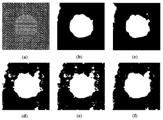
Figure 3.
Segmentation results on Image2. (a) original image; (b) AFWDLMO; (c) AFCMOMA; (d) AFCMDE; (e) MoMODEFC; (f) FCMNSGA.
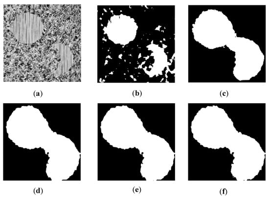
Figure 4.
Segmentation results on Image3. (a) original image; (b) AFWDLMO; (c) AFCMOMA; (d) AFCMDE; (e) MoMODEFC; (f) FCMNSGA.
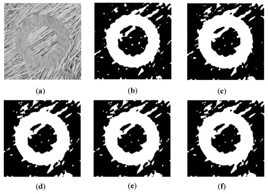
Figure 5.
Segmentation results on Image4. (a) original image; (b) AFWDLMO; (c) AFCMOMA; (d) AFCMDE; (e) MoMODEFC; (f) FCMNSGA.
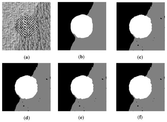
Figure 6.
Segmentation results on Image5. (a) original image; (b) AFWDLMO; (c) AFCMOMA; (d) AFCMDE; (e) MoMODEFC; (f) FCMNSGA.
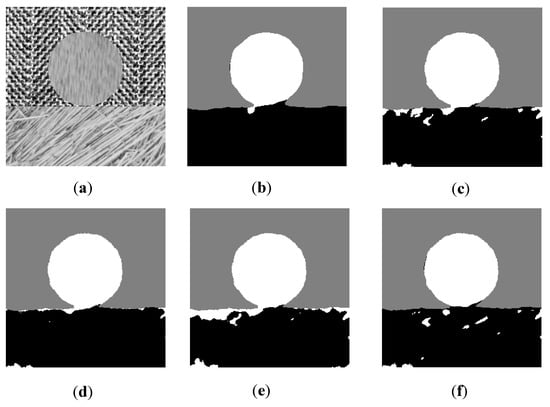
Figure 7.
Segmentation results on Image6. (a) original image; (b) AFWDLMO; (c) AFCMOMA; (d) AFCMDE; (e) MoMODEFC; (f) FCMNSGA.

Table 1.
Mean and variance of on texture images.
For the images of Gabor feature dominant, namely Image1 and Image2, the weights and obtained by the weight determination layer of AFWDLMO are positive, indicating that the weights of the Gabor feature are further increased. That is, AFWDLMO successfully recognizes that the two images are Gabor dominant. Table 1 statistically shows that AFWDLMO performs significantly better than the four competitors in terms of , indicating that the Gabor feature is fully utilized. In Figure 2 and Figure 3, it can be visually seen that AFWDLMO achieves the best segmentation accuracy, and AFCMOMA gives less misclassification than the other three algorithms.
For the images of GLCM feature dominant, namely Image3 and Image4, the weights and obtained by the weight determination layer of AFWDLMO are negative, respectively, which increases the weights of GLCM features. Similarly, AFWDLMO successfully recognizes that both Image3 and Image4 are GLCM dominant. As can be seen in Table 1, AFWDLMO outperforms other algorithms, particularly for Image3. Because the dimension of GLCM features is lower than that of Gabor features, when calculating the total similarity using the Euclidean distance, the Gabor feature with higher dimensions plays a decisive role in the computation, weakening the GLCM feature. Therefore, segmentation results are unsatisfied in all comparative algorithms. Figure 4 also visually presents that AFWDLMO achieves the best performance. AFWDLMO correctly classifies Image3 into two regions, while other algorithms misclassify the circles and crescents with the original isolated into a whole block. In Figure 5, all algorithms have similar segmentation results on Image4.
For Image5 and Image6, in theory, the segmentation results of Gabor features are slightly better than that of GLCM. As shown in Table 1, there is numerically no significant difference in all algorithms that achieve satisfactory segmentation results. The weights determined by AFWDLMO are and , respectively, which increases the effect of Gabor features on results. Therefore, the segmentation performance of AFWDLMO is slightly enhanced by positive weights. Figure 6 and Figure 7 also show that AFWDLMO is slightly superior to other algorithms.
4.2. Results on Texture Images with Speckle Noise
Due to the coherent imaging mechanism of SAR, SAR images are susceptible to speckle noise, which reduces the quality of SAR images and harms segmentation performance. In this section, as shown in Figure 8, two texture images (namely Image5 and Image6) with speckle noise (the mean is 0, the variance is 0.05 and 0.10 respectively) are used to demonstrate the ability of AFWDLMO to segment real SAR images. The segmentation on the texture images with speckle noise are shown in Figure 9, (a) is the original images, (b,c) are texture images with different speckle noise. Table 2 shows the results (mean and variance) of for texture images with different noises, the integer column of each case represents the optimal weights obtained by the weight determination layer, and the best result in each row is highlighted.
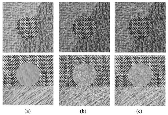
Figure 8.
Texture images with speckle noise. (a) Original images; (b) = 0.05; (c) = 0.10.
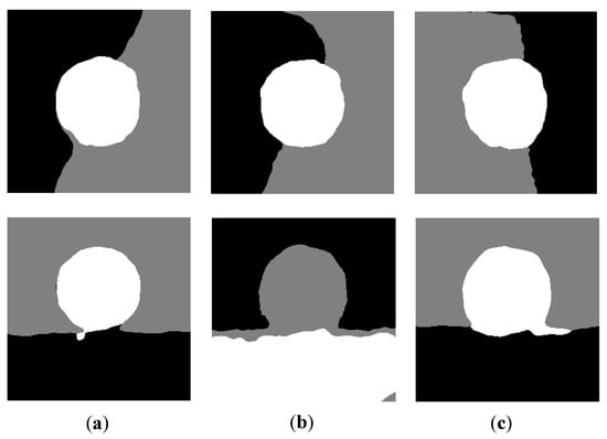
Figure 9.
Segmentation results on texture images with speckle noise. (a) original images; (b) = 0.05; (c) = 0.10.

Table 2.
Mean and variance of on texture images with speckle noise.
Compared to the segmentation results of the original image, there exists some misclassification on noise images due to the negative effect of speckle noise. For Image5, AFWDLMO gives the better segmentation results of var = 0.05 than that of var = 0.1. For Image6, AFWDLMO gives the better segmentation results of var = 0.10 than that of var = 0.05. As is seen in Table 2, the results of are worse than that of original images on two texture images with speckle noise. It is demonstrated that AFWDLMO can effectively suppress the speckle noise, but the segmentation accuracy is reduced by speckle noise.
4.3. Results on SAR Images
In this section, five algorithms are performed on eight real SAR images SAR1–SAR8 using the combination feature of gray and GLCM features. SAR5–SAR8 are available from https://www.sandia.gov/radar/ (accessed on 26 December 2021). Table 3 shows the four feature weights obtained from the weight determination layer of AFWDLMO. The final segmentation results are visually shown in Figure 10, Figure 11, Figure 12, Figure 13, Figure 14, Figure 15, Figure 16 and Figure 17, where (a) is the original SAR image, and (b–f) are segmentation results of five algorithms.

Table 3.
Feature weights obtained by AFWDLMO on eight SAR images.
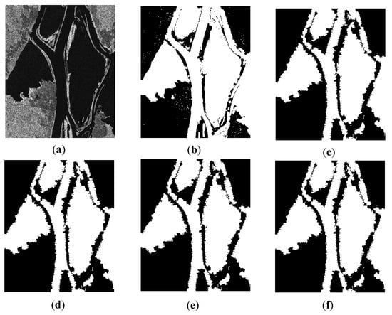
Figure 10.
Segmentation results on SAR1. (a) original image; (b) AFWDLMO; (c) AFCMOMA; (d) AFCMDE; (e) MoMODEFC; (f) FCMNSGA.
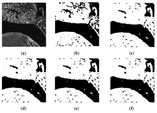
Figure 11.
Segmentation results on SAR2. (a) original image; (b) AFWDLMO; (c) AFCMOMA; (d) AFCMDE; (e) MoMODEFC; (f) FCMNSGA.
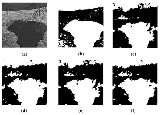
Figure 12.
Segmentation results on SAR3. (a) original image; (b) AFWDLMO; (c) AFCMOMA; (d) AFCMDE; (e) MoMODEFC; (f) FCMNSGA.
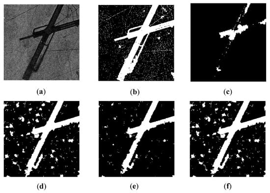
Figure 13.
Segmentation results on SAR4. (a) original image; (b) AFWDLMO; (c) AFCMOMA; (d) AFCMDE; (e) MoMODEFC; (f) FCMNSGA.
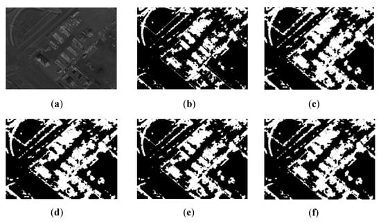
Figure 14.
Segmentation results on SAR5. (a) original image; (b) AFWDLMO; (c) AFCMOMA; (d) AFCMDE; (e) MoMODEFC; (f) FCMNSGA.
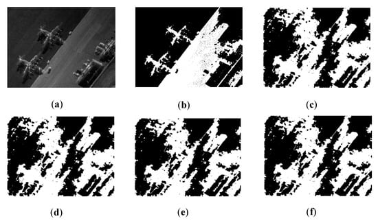
Figure 15.
Segmentation results on SAR6. (a) original image; (b) AFWDLMO; (c) AFCMOMA; (d) AFCMDE; (e) MoMODEFC; (f) FCMNSGA.
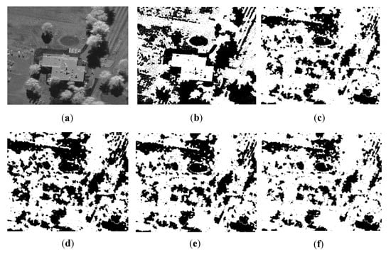
Figure 16.
Segmentation results on SAR7. (a) original image; (b) AFWDLMO; (c) AFCMOMA; (d) AFCMDE; (e) MoMODEFC; (f) FCMNSGA.
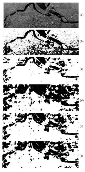
Figure 17.
Segmentation results on SAR8. (a) original image; (b) AFWDLMO; (c) AFCMOMA; (d) AFCMDE; (e) MoMODEFC; (f) FCMNSGA.
In Figure 10, SAR1 consists of two classes: lake (the white regions) and land (the black regions). AFWDLMO gives the best visual result, and the classifications of the lake and land are almost perfect. Although less misclassification in the land exists, only AFWDLMO perfectly maintains the curve of the lake bank compared to other algorithms. Other algorithms either deform the lake bank curve or lose pixels in the middle of lakes to be truncated to form many isolated small areas.
In Figure 11, SAR2 is classified into two regions: river (black regions) and land (white regions). AFWDLMO visibly achieves a better segmentation than the other algorithms, especially in the maintenance of the detailed structure and the river edge curve. In the middle of SAR2, the river is correctly classified in all algorithms because of the similar gray pixel and simple edge shape. In the land area below SAR2, all algorithms achieve less incorrect segmentation due to the similar gray pixel. For the land area in the upper left corner in SAR2, only AFWDLMO can accurately classify and preferably maintain the shape of the riverbank edge for each complex small lake structure, while other algorithms misclassify small lake areas into land areas. For the curved structure in the right of SAR2, four comparison algorithms merely obtain a whole area and lost lots of internal details. Nevertheless, AFWDLMO perfectly classifies the internal details in the curved structure, and the edge shape is consistent with the original image.
In Figure 12, SAR3 is classified into two areas: lake (white regions) and land (black regions). AFWDLMO is superior to others, and the lake edge curve is preferably maintained. In the land area, there is less misclassification for all five algorithms due to the inconsistency of the gray values. For the lake area, only AFWDLMO correctly classifies and maintains the shape of the lake bank edge. Other algorithms approximately classify SAR3 into the lake and land, but curves of the lake edge are seriously deformed.
In Figure 13, SAR4 mainly contains two classes: farmland (black regions) and runway (white regions). Compared with the four algorithms, AFWDLMO gives the best visual results, and each region is correctly classified except for some isolated pixels in the farmland. For the farmland, AFCMOMA outperforms other algorithms, followed by AFWDLMO with some isolated pixels, while the other three algorithms appear as large pixel blocks of misclassification. For the runway area, AFWDLMO perfectly performs the best segmentation. AFCMOMA is the worst because lots of breaks are occurred by much misclassification. In the other three algorithms, the main runway can be easily segmented, but it is difficult for the small branch of the runway to be classified. The three algorithms fail to segment efficiently, and misclassify these small branches as the farmland area.
In Figure 14, SAR5 mainly contains two classes: lands (black regions) and buildings (white regions). AFWDLMO gives the best visual results and maintains the edge details of each building, while the other four algorithms give slightly worse results.
In Figure 15, SAR6 can be classified into two classes: land (black regions) and airplane (white regions). Despite some mis-division existing in the results, AFWDLMO obtains a nice segmentation, which sensitively displays two airplanes on the left area and one airplane on the right area. The other four algorithms obtained the worst results, which show misclassification of large pixel blocks and can not maintain the details of airplanes. In addition, the split line (in the middle) is well seen in the result by AFWDLMO.
In Figure 16, SAR7 mainly shows a building, a pit on the land, and trees. It is visibly seen that AFWDLMO perfectly performs the best segmentation for the building area (white area) and the pit (black area), while other competitors merely maintain the shape of the pit. For AFWDLMO, the boundaries of different objects are clearly determined. In addition, all algorithms keep the shadows of trees (black area).
In Figure 17, SAR8 can be classified into two classes: the river (black regions) and land (white regions). It is visibly seen that AFWDLMO perfectly performs the best segmentation and AFCMDE the worst segmentation. Both AFWDLMO and AFCMOMA maintain the shape of the river edge, while both MoMODEFC and FCMNSGA roughly segment the river. Besides AFWDLMO, other competitors fail to keep details of a residential building on the land and give much misclassification.
Due to SAR imaging conditions, the boundaries of SAR are hard to be determined in many segmentation challenges. However, AFWDLMO outperforms all competitors on eight SAR images, which can determine the boundaries of different objects in SAR. Because the gray feature is dominant in eight SAR images, but its dimension is lower than the GLCM feature. When the Euclidean distance is used to calculate the total similarity, the GLCM feature with a high dimension plays a decisive role in the calculation, weakening the gray feature. That is, using the Euclidean distance reduces the impact of the gray feature on the segmentation. Consequently, segmentation results are unsatisfied in the comparison algorithms. AFWDLMO assigns an additional weight to the gray feature when calculating the similarity, which makes up for the reduction effect of the GLCM feature and enhances the performance of segmentation.
4.4. Analysis of Different Feature Weights
In this section, three images, namely Image1, Image3, and Image5, are selected to demonstrate the effectiveness of feature weights, where the Gabor feature is the first feature, and the GLCM feature is the second feature. To verify that the proposed AFWDLMO can adaptively adjust the feature weights for the different images, the weights determined by the weight determination layer and four fixed weights () are utilized in the clustering layer, respectively. Figure 18, Figure 19 and Figure 20 visually show the segmentation results using five different feature weights. Table 4 shows the results (mean and variance) of for the five feature weights, where the integer column of AFWDLMO represents the optimal weight obtained by the weight determination layer, and the best result in each row is highlighted.
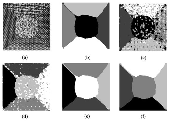
Figure 18.
Segmentation results of five different feature weights on Image1. (a) original image; (b) the weight of weight determination layer; (c) ; (d) ; (e) ; (f) .
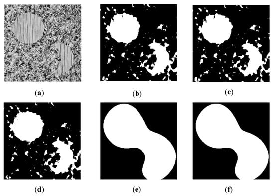
Figure 19.
Segmentation results of five different feature weights on Image3. (a) original image; (b) the weight of weight determination layer; (c) ; (d) ; (e) ; (f) .
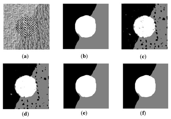
Figure 20.
Segmentation results of five different feature weights on Image5. (a) original image; (b) the weight of weight determination layer; (c) ; (d) ; (e) ; (f) .

Table 4.
Mean and variance of for five different feature weights.
For Image1, the weight determined by AFWDLMO is positive, which increases the weight of the Gabor feature. That is, AFWDLMO successfully recognizes that the Gabor feature is dominant. Table 4 shows that the results of with negative weights () are worse than using positive weights (, and 19 obtained by AFWDLMO). Figure 18e,f present that segmentation accuracy is extremely low using because the negative weights increase the weight of GLCM features and reduce the influence of the Gabor feature on the segmentation results. The segmentation performance decreases with the decrease of Gabor weights because Image1 is Gabor dominant. Similarly, increases the GLCM weight more than , which reduces the weight of Gabor features more than correspondingly. As a result, the results of are worse than . In addition, for , and the acquired weight 19, Figure 18 and Table 4 show that the result of is slightly better than , which indicates that segmentation results necessarily are not better as weights increase, but the best performance exists by an optimal weight. Furthermore, the result of is slightly better than and , which indicates that AFWDLMO can not only adaptively adjust the feature weights for images but also obtain optimal weights.
For Image3, the weight acquired by AFWDLMO is negative, which increases the weight of the GLCM feature. That is, AFWDLMO successfully recognizes that the GLCM feature is the dominant feature for Image3. Table 4 suggests that and with negative weights (, and the obtained weight ) are better than using positive weights (). Figure 19e,f show that segmentation accuracy is extremely low using the positive weights (), and the original isolated round and crescent are incorrectly divided into a whole block shown. The positive weights increase the weight of the Gabor feature such that it reduces the effect of the GLCM feature. In addition, the segmentation performance decreases with the decrease of GLCM weight because Image3 is GLCM dominant. Similarly to Image1, it is concluded that AFWDLMO can not only adaptively adjust the feature weight according to the image, but also obtain relatively better weight.
For Image5, the segmentation performance of Gabor is slightly better than that of GLCM. The positive weight determined by AFWDLMO improves the effect of the Gabor feature. In Table 4, it can be seen that the results of with positive weights are superior to positive weights. Moreover, Figure 20c,d visually show that the segmentation accuracy using the negative weights () is lower, and there is less incorrect segmentation. The result of AFWDLMO is slightly better than (), which shows that AFWDLMO can still assign weights to appropriate features, although Image5 theoretically is a similar segmentation effect between the Gabor feature and GLCM feature.
4.5. Analysis of the Proposed Algorithm
The computational complexity of AFWDLMO is , where G is the maximum number of generations during the evolution. Despite the proposed method having a high computational complexity, it gives the best results among all comparative methods. Therefore, the proposed deserves to be studied due to its satisfactory segmentation results.
Furthermore, for SAR images, the average time consumption of each algorithm in 20 runs is reported in Table 5, where it measures time by the second, and the best result in each row is highlighted. It is seen that the proposed method consumes a shorter time than other algorithms on three SAR images.

Table 5.
Average time consumption of each algorithm for SAR images.
5. Conclusions
In this paper, a two-layer framework is introduced for SAR image segmentation. Feature domination between two features is firstly defined; then, a discussion is that segmentation results are affected by the dimensions of feature weights. The segmentation accuracy is further improved by assigning additional weights to dominant features. In the first layer, a single objective problem is optimized by DE; then, an obtained optimal weight is transferred to the second layer. After receiving the feature weight, the two indices with the weight are optimized by MOEA/D to achieve satisfactory segmentation results on different images. The segmentation result on both texture images and real images suggests that the AFWDLMO achieves better segmentation results than other competitors. Additionally, the results of weights determined by the first layer and several fixed weights confirm that AFWDLMO can identify the dominant feature and obtain its optimal weights adaptively.
Author Contributions
Conceptualization, R.L.; methodology, R.L.; validation, M.X.; formal analysis, H.L.; investigation, M.X.; resources, H.L.; writing—original draft preparation, M.X.; writing—review and editing, H.L.; funding acquisition, R.L. All authors have read and agreed to the published version of the manuscript.
Funding
This work was supported by the National Natural Science Foundation of China (Nos. 61876141 and 61373111), and the Provincial Natural Science Foundation of Shaanxi of China (No. 2019JZ-26).
Conflicts of Interest
The authors declare no conflict of interest.
References
- Wang, F.; Wu, Y.; Li, M.; Zhang, P.; Zhang, Q. Adaptive Hybrid Conditional Random Field Model for SAR Image Segmentation. IEEE Trans. Geosci. Remote Sens. 2017, 55, 537–550. [Google Scholar] [CrossRef]
- Xiang, D.; Zhang, F.; Zhang, W.; Tang, T.; Guan, D.; Zhang, L.; Su, Y. Fast Pixel-Superpixel Region Merging for SAR Image Segmentation. IEEE Trans. Geosci. Remote Sens. 2021, 59, 9319–9335. [Google Scholar] [CrossRef]
- Liu, C.; Bian, T.; Zhou, A. Multiobjective multiple features fusion: A case study in image segmentation. Swarm Evol. Comput. 2021, 60, 100792. [Google Scholar] [CrossRef]
- Bezdek, J.C.; Ehrlich, R.; Full, W. FCM: The fuzzy c-means clustering algorithm. Comput. Geosci. 1984, 10, 2–3. [Google Scholar] [CrossRef]
- Xu, Z.; Wu, J. Intuitionistic fuzzy c-means clustering algorithms. J. Syst. Eng. Electron. 2010, 21, 580–590. [Google Scholar] [CrossRef]
- Lin, K. A novel evolutionary kernel intuitionistic fuzzy c-means clustering algorithm. IEEE Trans. Fuzzy Syst. 2014, 22, 1074–1087. [Google Scholar] [CrossRef]
- Verma, H.; Agrawal, R.; Sharan, A. An improved intuitionistic fuzzy c-means clustering algorithm incorporating local information for brain image segmentation. Appl. Soft Comput. 2016, 46, 543–557. [Google Scholar] [CrossRef]
- Arshad, A.; Riaz, S.; Jiao, L.; Murthy, A. A semi-supervised deep fuzzy c-mean clustering for two classes classification. In Proceedings of the 2007 IEEE 3rd Information Technology and Mechatronics Engineering Conference (ITOEC), Chongqing, China, 3–5 October 2017; pp. 365–370. [Google Scholar]
- Ahmed, M.N.; Yamany, S.M.; Mohamed, N.; Farag, A.A.; Moriarty, T. A modified fuzzy c-means algorithm for bias field estimation and segmentation of MRI data. IEEE Trans. Med. Imaging 2002, 21, 193–199. [Google Scholar] [CrossRef]
- Chen, S.; Zhang, D. Robust image segmentation using FCM with spatial constraints based on new kernel-induced distance measure. IEEE Trans. Syst. Man Cybern. Part B 2004, 34, 1907–1916. [Google Scholar] [CrossRef]
- Szilagyi, L.; Benyo, Z.; Szilagyi, S.M.; Adam, H.S. MR brain image segmentation using an enhanced fuzzy c-means algorithm. In Proceedings of the 25th Annual International Conference of the IEEE Engineering in Medicine and Biology Society (IEEE Cat. No. 03CH37439), Cancun, Mexico, 17–21 September 2003; Volume 1, pp. 724–726. [Google Scholar]
- Cai, W.; Chen, S.; Zhang, D. Fast and robust fuzzy c-means clustering algorithms incorporating local information for image segmentation. Pattern Recognit. 2007, 40, 825–838. [Google Scholar] [CrossRef]
- Krinidis, S.; Chatzis, V. A Robust Fuzzy Local Information c-Means Clustering Algorithm. IEEE Trans. Image Process. 2010, 19, 1328–1337. [Google Scholar] [CrossRef] [PubMed]
- Shang, R.; Tian, P.; Jiao, L.; Stolkin, R.; Feng, J.; Hou, B.; Zhang, X. A Spatial Fuzzy Clustering Algorithm with Kernel Metric Based on Immune Clone for SAR Image Segmentation. IEEE J. Sel. Top. Appl. Earth Obs. Remote Sens. 2016, 9, 1640–1652. [Google Scholar] [CrossRef]
- Goldberg, D.E. Genetic Algorithms in Search, Optimization and Machine Learning, 1st ed.; Addison-Wesley Longman Publishing Company Inc.: Boston, MA, USA, 1989. [Google Scholar]
- Fogel, D.B. Natural Evolution. In IEEE Press Series on Computational Intelligence; Evolutionary Computation: Toward a New Philosophy of Machine Intelligence; John Wiley & Sons: Piscataway, NJ, USA, 2006; pp. 33–58. [Google Scholar]
- Fogel, D.B. Theoretical and Empirical Properties of Evolutionary Computation. In IEEE Press Series on Computational Intelligence: Evolutionary Computation||Theoretical and Empirical Properties of Evolutionary Computation; John Wiley & Sons: Piscataway, NJ, USA, 2006; pp. 105–181. [Google Scholar] [CrossRef]
- Jiao, L.; Gong, M.; Wang, S.; Hou, B.; Zheng, Z.; Wu, Q. Natural and Remote Sensing Image Segmentation Using Memetic Computing. IEEE Comput. Intell. Mag. 2010, 5, 78–91. [Google Scholar] [CrossRef]
- Maulik, U.; Saha, I. Automatic Fuzzy Clustering Using Modified Differential Evolution for Image Classification. IEEE Trans. Geosci. Remote Sens. 2010, 48, 3503–3510. [Google Scholar] [CrossRef]
- Ma, M.; Liang, J.; Guo, M.; Fan, Y.; Yin, Y. SAR image segmentation based on artificial bee colony algorithm. Appl. Soft Comput. 2011, 11, 5205–5214. [Google Scholar] [CrossRef]
- Khan, A.; Jaffar, M.A. Genetic algorithm and self-organizing map based fuzzy hybrid intelligent method for color image segmentation. Appl. Soft Comput. 2015, 32, 300–310. [Google Scholar] [CrossRef]
- Khan, A.; Jaffar, M.A.; Shao, L. A modified adaptive differential evolution algorithm for color image segmentation. Knowl. Inf. Syst. 2015, 43, 583–597. [Google Scholar] [CrossRef]
- Paoli, A.; Melgani, F.; Pasolli, E. Clustering of Hyperspectral Images Based on Multiobjective Particle Swarm Optimization. IEEE Trans. Geosci. Remote Sens. 2009, 47, 4175–4188. [Google Scholar] [CrossRef]
- Handl, J.; Knowles, J. Evolutionary multiobjective clustering. Parallel Probl. Solving Nat. 2004, 3242, 1081–1091. [Google Scholar]
- Corne, D.; Jerram, N.; Knowles, J.; Oates, M.J. PESA-II: Region-based selection in evolutionary multiobjective optimization. In Proceedings of the GECCO Annual Conference on Genetic and Evolutionary Computation, San Francisco, CA, USA, 7–11 July 2001. [Google Scholar]
- Handl, J.; Knowles, J. An Evolutionary Approach to Multiobjective Clustering. IEEE Trans. Evol. Comput. 2007, 11, 56–76. [Google Scholar] [CrossRef]
- Bandyopadhyay, S.; Maulik, U.; Mukhopadhyay, A. Multiobjective Genetic Clustering for Pixel Classification in Remote Sensing Imagery. IEEE Trans. Geosci. Remote Sens. 2007, 45, 1506–1511. [Google Scholar] [CrossRef]
- Deb, K.; Pratap, A.; Agarwal, S.; Meyarivan, T. A fast and elitist multiobjective genetic algorithm: NSGA-II. IEEE Trans. Evol. Comput. 2002, 6, 182–197. [Google Scholar] [CrossRef]
- Yang, D.; Jiao, L.; Gong, M.; Liu, F. Artificial immune multi-objective SAR image segmentation with fused complementary features. Inf. Sci. 2011, 181, 2797–2812. [Google Scholar] [CrossRef]
- Zhong, Y.; Zhang, S.; Zhang, L. Automatic Fuzzy Clustering Based on Adaptive Multi-Objective Differential Evolution for Remote Sensing Imagery. IEEE J. Sel. Top. Appl. Earth Obs. Remote Sens. 2013, 6, 2290–2301. [Google Scholar] [CrossRef]
- Xie, X.L.; Beni, G. A validity measure for fuzzy clustering. IEEE Trans. Pattern Anal. Mach. Intell. 1991, 13, 841–847. [Google Scholar] [CrossRef]
- Ma, A.; Zhong, Y.; Zhang, L. Adaptive Multiobjective Memetic Fuzzy Clustering Algorithm for Remote Sensing Imagery. IEEE Trans. Geosci. Remote Sens. 2015, 53, 4202–4217. [Google Scholar] [CrossRef]
- Storn, R.; Price, K. Differential Evolution—A Simple and Efficient Heuristic for global Optimization over Continuous Spaces. J. Glob. Optim. 1997, 45, 341–359. [Google Scholar] [CrossRef]
- Gao, B.; Wang, J. Multi-Objective Fuzzy Clustering for Synthetic Aperture Radar Imagery. IEEE Geosci. Remote Sens. Lett. 2015, 12, 2341–2345. [Google Scholar] [CrossRef]
- Zhao, F.; Liu, H.; Fan, J. A multiobjective spatial fuzzy clustering algorithm for image segmentation. Appl. Soft Comput. 2015, 30, 48–57. [Google Scholar] [CrossRef]
- Zhang, M.; Jiao, L.; Ma, W.; Ma, J.; Gong, M. Multi-objective evolutionary fuzzy clustering for image segmentation with MOEA/D. Appl. Soft Comput. 2016, 48, 621–637. [Google Scholar] [CrossRef]
- Zhang, Q.; Li, H. MOEA/D: A Multiobjective Evolutionary Algorithm Based on Decomposition. IEEE Trans. Evol. Comput. 2007, 11, 712–731. [Google Scholar] [CrossRef]
- Saha, I.; Maulik, U.; Plewczynski, D. A new multi-objective technique for differential fuzzy clustering. Appl. Soft Comput. 2011, 11, 2765–2776. [Google Scholar] [CrossRef]
- Wikaisuksakul, S. A multi-objective genetic algorithm with fuzzy c-means for automatic data clustering. Appl. Soft Comput. 2014, 24, 679–691. [Google Scholar] [CrossRef]
- Sun, Z.; Geng, H.; Lu, Z.; Scherer, R.; Wozniak, M. Review of Road Segmentation for SAR Images. Remote Sens. 2021, 13, 1011. [Google Scholar] [CrossRef]
- Duan, Y.; Liu, F.; Jiao, L.; Zhao, P.; Zhang, L. SAR Image segmentation based on convolutional-wavelet neural network and markov random field. Pattern Recognit. 2017, 64, 255–267. [Google Scholar] [CrossRef]
- Mallat, S.G. A Theory for Multiresolution Signal Decomposition: The Wavelet Representation. IEEE Trans. Pattern Anal. Mach. Intell. 1989, 11, 674–693. [Google Scholar] [CrossRef]
- Saneva, W.; Vindas, J. Wavelet expansions and asymptotic behavior of distributions. J. Math. Anal. Appl. 2010, 370, 543–554. [Google Scholar] [CrossRef]
- He, C.; Li, S.; Liao, Z.; Liao, M. Texture classification of PolSAR data based on sparse coding of wavelet polarization textons. IEEE Trans. Geosci. Remote Sens. 2013, 51, 4576–4590. [Google Scholar] [CrossRef]
- Guariglia, E.; Silvestrov, S. Fractional-Wavelet Analysis of Positive definite Distributions and Wavelets on D’(C). Eng. Math. II 2016, 179, 337–353. [Google Scholar]
- Heydari, M.H. Chebyshev cardinal wavelets for nonlinear variable-order fractional quadratic integral equations. Appl. Numer. Math. 2019, 144, 190–203. [Google Scholar] [CrossRef]
- Bi, H.; Xu, L.; Cao, X.; Xue, Y.; Xu, Z. Polarimetric SAR Image Semantic Segmentation With 3D Discrete Wavelet Transform and Markov Random Field. IEEE Trans. Image Process. 2020, 29, 6601–6614. [Google Scholar] [CrossRef]
- Xia, J.; Yokoya, N.; Adriano, B.; Zhang, L.; Li, G.; Wang, Z. A Benchmark High-Resolution GaoFen-3 SAR Dataset for Building Semantic Segmentation. IEEE J. Sel. Top. Appl. Earth Obs. Remote Sens. 2021, 14, 5950–5963. [Google Scholar] [CrossRef]
- Coello, C.A.C.; Lamont, G.B.; Van Veldhuizen, D.A. Evolutionary Algorithm for Solving Multi-Objective Problems; Springer: Berlin/Heidelberg, Germany, 2007. [Google Scholar]
- Wang, J.; Liang, G.; Zhang, J. Cooperative Differential Evolution Framework for Constrained Multiobjective Optimization. IEEE Trans. Cybern. 2019, 49, 2060–2072. [Google Scholar] [CrossRef] [PubMed]
- Xiao, X.; Zhou, Y.; Gong, Y. Content-Adaptive Superpixel Segmentation. IEEE Trans. Image Process. 2018, 27, 2883–2896. [Google Scholar] [CrossRef] [PubMed]
- Chuchvara, A.; Gotchev, A. Content-Adaptive Superpixel Segmentation Via Image Transformation. In Proceedings of the 2019 IEEE International Conference on Image Processing (ICIP), Taipei, Taiwan, 22–25 September 2019; pp. 1505–1509. [Google Scholar]
- Meyer, F. An Overview of Morphological Segmentation. Int. J. Pattern Recognit. Artif. Intell. 2001, 15, 1089–1118. [Google Scholar] [CrossRef]
- Kanopoulos, N.; Vasanthavada, N.; Baker, R.L. Design of an image edge detection filter using the Sobel operator. IEEE J. Solid-State Circuits 1998, 23, 358–367. [Google Scholar] [CrossRef]
- Cong, A.; Cong, W.; Lu, Y.; Santago, P.; Chatziioannou, A.; Wang, G. Differential evolution approach for regularized bioluminescence tomography. IEEE Trans. Biomed. Eng. 2010, 57, 2229–2238. [Google Scholar] [CrossRef]
- Rekanos, I.T. Shape Reconstruction of a Perfectly Conducting Scatterer Using Differential Evolution and Particle Swarm Optimization. IEEE Trans. Geosci. Remote Sens. 2008, 46, 1967–1974. [Google Scholar] [CrossRef]
- Liu, H.; Li, X.; Gong, W. Rethinking the differential evolution algorithm. Serv.-Oriented Comput. Appl. 2020, 14, 79–87. [Google Scholar] [CrossRef]
- Das, S.; Suganthan, P.N. Differential Evolution: A Survey of the State-of-the-Art. IEEE Trans. Evol. Comput. 2011, 15, 4–31. [Google Scholar] [CrossRef]
- Pakhira, M.; Bandyopadhyay, S.; Maulik, U. Validity index for crisp and fuzzy clusters. Pattern Recognit. 2004, 37, 487–501. [Google Scholar] [CrossRef]
- Santos, J.; Embrechts, M. On the use of the adjusted rand index as a metric for evaluating supervised classification. Artif. Neural Netw. ICANN 2009, 5769, 175–184. [Google Scholar]
Publisher’s Note: MDPI stays neutral with regard to jurisdictional claims in published maps and institutional affiliations. |
© 2022 by the authors. Licensee MDPI, Basel, Switzerland. This article is an open access article distributed under the terms and conditions of the Creative Commons Attribution (CC BY) license (https://creativecommons.org/licenses/by/4.0/).