Abstract
Because canola is a major oilseed crop, accurately determining its planting areas is crucial for ensuring food security and achieving UN 2030 sustainable development goals. However, when canola is extracted using remote-sensing data, winter wheat causes serious interference because it has a similar growth cycle and spectral reflectance characteristics. This interference seriously limits the classification accuracy of canola, especially in mixed planting areas. Here, a novel canola flower index (CFI) is proposed based on the red, green, blue, and near-infrared bands of Sentinel-2 images to improve the accuracy of canola mapping, based on the finding that spectral reflectance of canola on the red and green bands is higher than that of winter wheat during the canola flowering period. To investigate the potential of the CFI for extracting canola, the IsoData, support vector machine (SVM), and random forest (RF) classification methods were used to extract canola based on Sentinel-2 raw images and CFI images. The results show that the average overall accuracy and kappa coefficient based on CFI images were 94.77% and 0.89, respectively, which were 1.05% and 0.02, respectively, higher than those of the Sentinel-2 raw images. Then we found that a threshold of 0.14 on the CFI image could accurately distinguish canola from non-canola vegetation, which provides a solution for automatic mapping of canola. The overall classification accuracy and kappa coefficient of this threshold method were 96.02% and 0.92, which were very similar to those of the SVM and RF methods. Moreover, the advantage of the threshold classification method is that it reduces the dependence on training samples and has good robustness and high classification efficiency. Overall, this study shows that CFI and Sentinel-2 images provide a solution for automatic and accurate canola extraction.
1. Introduction
Canola (Brassica napus L.) is one of the major oilseed crops worldwide. It is the primary source of edible oil for human consumption and a biological feedstock for fuels [1]. Canola flowers are an important tourism resource, promoting the local development of tourism agriculture [2,3]. However, the production and consumption of canola are unbalanced in different world regions. For example, China’s domestic canola production is far less than its increasing demand for canola [2]. Mapping and tracking the unbalance in canola planting areas is of great importance for agricultural management and food security.
Remote-sensing technology has made significant progress in efficiently mapping crops because of its low cost, comprehensive coverage, and regular acquisition [4,5,6]. Crop mapping methods that use remote-sensing technology vary in complexity, from clustering [7], decision trees [8], and object-oriented methods [9] to machine learning methods [10]. Most previous studies of crop identification have relied mainly on the availability of well-represented training-data samples [11,12]. The provision of such training-data is usually time-consuming, costly, and labor-intensive. Also, methods with specific training data might be subject to low cross-year or different-region repeatability [13]. Consequently, it is urgent to improve the automation level and robustness of crop mapping.
Enhanced imagery of crop characteristics gleaned from their phenological information helps detect and map crops automatically [14,15]. These characteristics are exclusive and steady because most crops show a unique phenological pattern, even though some have a similar growing season [16,17]. Hence, once an automated algorithm derived from these characteristics is completed and published, it can provide training rules that can be used directly and repeated year after year without retraining [13,18]. Several previous studies have successfully used phenology-derived characteristics for automatic mapping of crops [13,19].
In the past, the mapping of canola did not receive enough attention [3]. In recent years, with the continuous rise in the economic value of canola, several studies have begun to pay attention to the remote sensing of canola. For example, d’Andrimont et al. [20] and Mercier et al. [21] mapped canola flowering phenology in parts of Germany and France, respectively. Tao et al. [22] mapped the spatiotemporal dynamics of canola on the Jianghan Plain and the Dongting Lake Plain in China. Han et al. [23] published a data product for canola mapping from 2017 to 2019 in 33 countries based on Sentinel satellite images. However, the data produced did not include China.
One of the challenges of canola remote-sensing identification is that winter wheat and canola have similar growth cycles and spectral reflectance characteristics during their entire growing season [14]. In China, the distribution of canola fields and winter wheat fields is usually staggered and mixed. This further increases the difficulty of canola identification by remote-sensing images. Fortunately, the phenological characteristics of canola flowers provide an opportunity to distinguish between canola and winter wheat, even though the flowering period is transitory; only 1 month, approximately. Several studies have attempted to map canola by detecting its bright yellow flowers using remote-sensing images [24]. For instance, Fang et al. [25] proposed a simple model for estimating canola flowers during the canola flowering season. Sulik and Long [3] proposed the green/blue band ratio to identify canola flowers. Later, Sulik and Long [1] further proposed a normalized difference yellowness index (NDYI) to estimate canola yields. Ashourloo et al. [11] proposed a canola index (CI) during the flowering period, computed as the near-infrared (NIR) band multiplied by the sum of red and green bands. Previous studies have gradually enriched and improved the canola indices.
Coarse imagery, such as that of MODIS and Landsat, can barely detect the actual boundaries of farmland. However, high-resolution sensors such as Sentinel-2 have sufficient spatial resolution for canola mapping. Image data volume is closely related to spatial resolution [10]. Therefore, a flood of data are encountered when analyzing Sentinel-2 images. The cloud computing platform of the Google Earth Engine (GEE), however, provides a solution for processing very large amounts of massive remote-sensing data [26]. The GEE stores entire data products from major international remote-sensing satellites, such as Sentinel, and has good data-management practices [27].
In this study, the objectives were to (1) characterize the spectral reflectance of canola at a canopy scale during the canola flowering stage, (2) build a novel canola flower index (CFI) for automatic canola mapping, and (3) achieve automatic identification of canola on the GEE.
2. Materials and Methods
2.1. Study Area
For this study, three study areas were selected, as shown in Figure 1. The first was in Wuxue County, in the east of Hubei Province, China; the second in Hanzhong County, in Shanxi Province, China; and the third in Hanshou County and its surrounding areas, in Hunan Province, China. The first study area was used to investigate the spectral reflectance of various objects and construct the CFI. The other two study areas were then used to validate the effectiveness of the CFI. On remote-sensing imagery, canola fields and winter wheat fields have a mosaic or crisscross distribution. The canola fields are highly fragmented, and their areas are generally less than 1 hectare. In addition, canola and winter wheat have a similar growth cycle from October to May [28]. Those phenomena increased the challenge of remotely sensing canola in those study areas.
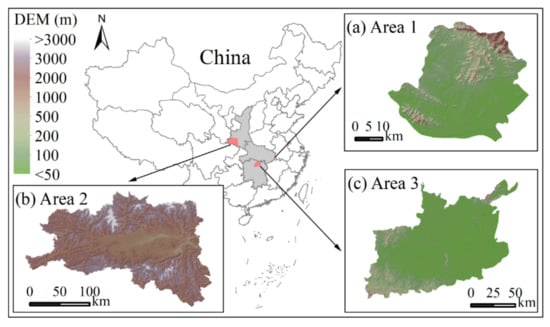
Figure 1.
Locations of the study areas. (a) The first study area, Hubei Province. (b) The second study area, Shanxi Province. (c) The third study area, Hunan Province.
The phenological calendar of canola and winter wheat in those study areas was investigated, as shown in Figure 2. Canola and wheat were usually sown in October. Canola generally enters the flowering stage in May, when winter wheat enters the stem-elongation stage. In May, both enter the mature stage.

Figure 2.
Phenological calendar of canola and winter wheat. F, M, and L represent the first, middle, and last 10 d of a month, respectively.
2.2. Sentinel-2 Imagery
The Sentinel-2 satellite was launched by the European Commission and European Space Agency [29]. Sentinel-2 images cover 13 wavebands [30,31]. The red, green, blue, and NIR wavebands have a spatial resolution of 10 m. The four red-edge wavebands and two shortwave infrared wavebands have a spatial resolution of 20 m. The spatial resolution of the other three wavebands is 60 m. Their revisit period is 10 d. In this study, the red, green, blue, and NIR wavebands were used because their spatial resolution is high. In addition, according to previous research [17,32], the red-edge wavebands with a spatial resolution of 20 m contribute little to improving the identification accuracy of canola.
In accordance with the principle of no cloud coverage, we selected six-phase Sentinel-2 images covering the first study area to investigate the spectral reflectance of various types of ground objects, such as canola, winter wheat, forest, bare land, and construction land. The imaging dates for the six-phase Sentinel-2 images are shown in Table 1. Those dates covered the main growth stages of canola—seedling, wintering, budding, flowering, silique, and mature—as shown in Figure 2.

Table 1.
Dates of Sentinel-2 images used in the study.
In the second and third study areas, those Sentinel-2 images were selected during the canola flowering stage because those two study areas were used to validate the effectiveness of the CFI. The imaging dates are shown in Table 1.
All Sentinel-2 images used in the study came from the imagery collection “COPERNICUS/S2_SR” on the GEE platform. Those images were surface reflectance data, which were atmospheric corrected [33,34].
2.3. Confirming the Optimum Period
During canola’s flowering period, canola fields and winter wheat fields have a significant visual difference; canola fields are yellow, and winter wheat fields are green. To confirm the specific optimum period in this study, the Fisher function of the spectrum between canola and other ground objects in various phases was computed. The Fisher function is [11]:
where m and v are the mean and variance values of spectral reflectance, respectively, and subscripts 1 and 2 represent two different categories.
The Fisher value describes the difference between the classes. The greater the Fisher value, the greater the separability between categories. By using 3256 sets of pixel samples for each spectrum (i.e., the red, green, blue, and NIR wavebands), the Fisher values between canola and wheat, forest, bare land, and construction land were computed in various phases: 11 November 2019, 6 December 2019, 9 February 2020, 20 March 2020, 29 April 2020, and 19 May 2020. The phase with the maximum Fisher value was the optimum period for canola mapping.
2.4. Building the Canola Flower Index
The spectral reflectance of various ground objects during the canola flowering period was plotted based on Sentinel-2 images, as shown in Figure 3. The spectral data were obtained by using ENVI software based on Sentinel-2 images. There were five ground objects, i.e., canola, wheat, forest, construction land, and bare land. The imagery layers were the red, green, blue, NIR, and normalized difference vegetation index (NDVI). The NDVI has the potential to distinguish between canola and no-vegetation objects [35,36]. In Figure 3, the NDVI value of construction land and bare land is less than 0.2, whereas that of canola is more than 0.5. The NDVI value range of canola does not overlap with that of other objects. The difference between canola and construction land, canola, and bare land is significant in the NDVI band. Therefore, NDVI was taken as a component of the CFI.
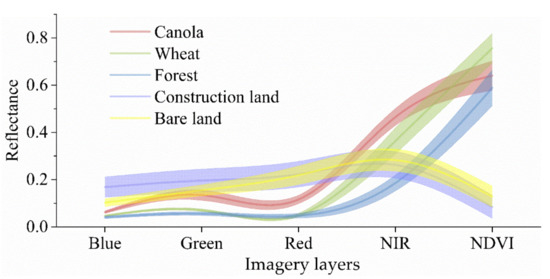
Figure 3.
Spectral reflectance of various ground objects in Sentinel-2 imagery dated 20 March 2020 in the first study area. That imaging date was the canola flowering period.
The difference in spectral reflectance between canola and wheat, canola, and forest was discernable in the green and red bands, as shown in Figure 3. Therefore, two features could be constructed to expand this difference in spectral reflectance. First, the sum of the red and green band reflectance for canola was greater than that for wheat and forest. Second, the difference in spectral reflectance between the green and blue bands for canola was greater than that for wheat and forest. Considering the NDVI, three features were obtained for building the CFI. Different combination patterns of those three features were used to construct different CFIs. This combination sequence was that (a) The three features were added, (b) the three features were multiplied, (c) the sum of any two features was multiplied with the third feature, and (d) the product of any two features was added to the third feature. Thereby, eight CFIs were constructed.
To find the best CFI of the eight CFIs, the Fisher value between canola and wheat, forest, bare land, and construction land for each CFI equation was compared by using the same samples, respectively. Those samples were 5219 pixels, which came from the three study areas. The CFI with the highest Fisher value was considered the optimal CFI.
2.5. Classification Methods
To verify whether the optimal CFI enhances the image features of the canola compared to Sentinel-2 raw images, canola was extracted based on the Sentinel-2 raw images and the optimal CFI image derived from the Sentinel-2 raw images. This was done by using an unsupervised classification method (i.e., the IsoData cluster method [37,38]), and two supervised classification methods (i.e., support vector machine (SVM) [39,40] and random forest (RF) [41]). Because IsoData is hardly affected by subjective human factors, and classification is automatically done by computers based on the characteristics of the image itself, the classification results from IsoData could determine to some extent whether the optimal CFI images were better than the raw images. The SVM and RF classifiers are widely used within the remote sensing community because of the accuracy of their classification [39,41]. Therefore, IsoData, SVM, and RF classifiers were selected to evaluate the performance of the CFI in the study. The training samples were the same when extracting canola by different classifiers based on the CFI images and Sentinel-2 raw images. The testing samples were the same for evaluating different classification results derived from different classifiers.
A decision tree model [42] was built in GEE to improve the automation level and robustness of the canola mapping. Specifically, the CFI values of canola had more than one threshold. For the optimal CFI images during the optimum period, we count and analyze the histogram of CFI values by 3517 canola and 3517 non-canola pixels in the first study area to confirm a preset threshold. Due to the preset threshold being obtained from the samples in the first study area, it was necessary to further verify the stability and reliability of the preset threshold in other regions. Therefore, the data surrounding the preset threshold were taken one by one as the judgment threshold to distinguish between canola and non-canola. Then the accuracies of the classification results were compared by using the confusion matrix accuracy verification method [43,44] and all validation samples in the three study areas. The threshold corresponding to the highest accuracy was the best judgment threshold required by the model. The rule of threshold traversal was to gradually move five steps, with 0.01 interval, to the left and right sides of the preset threshold. Thus, the best threshold was selected from the 11 candidate thresholds according to their performance in the classification results.
Then the classification accuracies of the decision tree model, SVM, and RF methods were compared in the three study areas. The primary purpose was to test whether the decision tree model was better than the SVM or RF classifier for canola mapping. Another purpose was to test the applicability of the decision tree model because training samples were not used in the second and third study areas. If the classification accuracy of the decision tree model was satisfactory in the second and third study areas, automatic identification of canola would have been achieved without relying on training samples.
2.6. Accuracy Verification
In the study, 45 validation quadrats with dimensions of 0.5 km × 0.5 km were randomly selected. Three steps were taken to complete the production of those validation quadrats, as shown in Figure 4. First, the boundaries of various ground objects within each validation quadrat were manually plotted in accordance with Google imagery with a spatial resolution of 0.1 m × 0.1 m. Second, the vector data attributes for different ground objects were determined and labeled from field-based survey data. The canola fields were labeled as “canola” type, and all other ground objects were labeled as “other” type. Third, the vector data were converted to raster data, and their spatial resolution was converted to 10 m, the same as the classification results. Those raster data were regarded as the ground-truth samples. Then the confusion matrix accuracy verification method [43,44] and F1 score [45] were used to verify the classification accuracy. The confusion matrix accuracy parameters included overall accuracy, production accuracy, user accuracy, and the kappa coefficient.
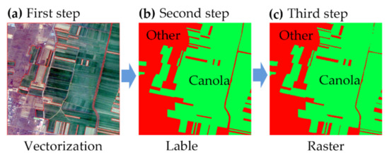
Figure 4.
The validation quadrats data production process. (a) The Google imagery base map with a spatial resolution of 0.1 m × 0.1 m, and the red lines are the vectorized boundaries of different objects. (b) The green vector data are canola fields, and the red areas represent other objects. (c) The raster data derived from the second step.
2.7. Comparison of CFI with Other Canola Indices
Some canola indices have been used for canola identification in previous studies. For example, Sulik and Long proposed a canola ratio index (CRI) [3] and a normalized difference yellowness index (NDYI) [1]. Ashourloo et al. [11] proposed a canola index (CI). The equations are as follows:
where βgreen, βblue, βred, and βnir represent the spectral reflectance on green, blue, red, and near-infrared wavebands, respectively.
In order to compare the performance of the CFI proposed in this study with those existing canola indices, i.e., CRI, NDYI, and CI, their classification accuracies based on different classification method were also obtained in the study.
3. Results
3.1. Optimum Period
The Fisher values of the canola and other ground objects in the four wavebands and NDVI images during the canola growth period in the first study area were plotted in Figure 5.
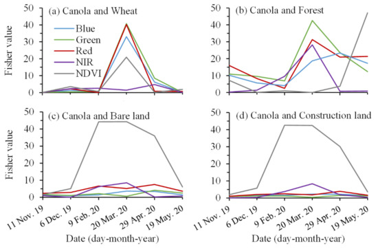
Figure 5.
Fisher values (a) between canola and wheat, (b) between canola and forest, (c) between canola and bare land, and (d) between canola and construction land in different spectral bands from 11 November 2019 to 19 May 2020 in the first study area.
Note that March is the flowering period for canola. In Figure 5a, on 20 March 2020, the Fisher values between canola and wheat in the blue, green, and red wavebands reached the peak values of 33.02, 40.75, and 40.21, respectively. Those values were approximately seven times higher than those in other periods. The Fisher values between canola and wheat in the NDVI layer also reached a peak value of 20.95 on 20 March 2020. For the NIR band, the Fisher values between canola and winter wheat were low throughout the growth period, fluctuating around 2.86. In Figure 5b, the green and red wavebands still performed well in distinguishing canola from forest, and their Fisher values were 42.58 and 31.31, respectively, on 20 March 2020. The Fisher value on the blue waveband was 18.74. As shown in Figure 5c,d, the NDVI image had an absolute advantage in identifying canola on 20 March 2020 compared to the four wavebands. Because the Fisher values of the NDVI were greater than 40, whereas the Fisher values of the four wavebands were less than 10 on 20 March 2020. Those results demonstrated that the blue, green, and red wavebands, and NDVI layer of the Sentinel-2 image on 20 March 2020 had the best potential to identify canola.
In the same way, on 20 March 2020, the Fisher values between canola and other ground objects were high. Those results proved that the Sentinel-2 image on 20 March 2020 had the best potential to identify canola. Therefore, Sentinel-2 images during canola flowering were used to map canola.
3.2. Optimum Canola Flower Index
In accordance with the three features for building the CFI (Section 2.4), eight canola flower indices were derived:
where sumred, green is the sum of spectral reflectance on the red and green spectral wavebands, and diffgreen, blue is the difference between the green and blue spectral wavebands.
where βred, βgreen, βblue, and βnir are the spectral reflectance on red, green, blue, and NIR wavebands, respectively.
For the different CFI images on 20 March 2020, the Fisher values between canola and the other four types of ground objects are shown in Table 2.

Table 2.
Fisher values of canola and other ground objects for various CFIs.
The mean Fisher value of CFI3 was 44.81, which was maximal. Also, CFI3 gave canola and all other objects good separability. For example, although the Fisher value between canola and wheat was minimal compared to other objects, the value was as high as 34.51. For the CFI3, it was multiplied by two factors, as shown in Equation (7). The first factor was NDVI, which can distinguish between non-vegetation. Because the NDVI values of non-vegetation were less than 0.2, whereas canola was more than 0.5, as shown in Figure 3. In addition, the second factor values of canola were greater than that of non-vegetation. Therefore, CFI3 can accurately distinguish canola from non-vegetation. Although the NDVI values of wheat and forest were similar to those of canola, the second factor values of canola were greater than those of wheat and forest. Therefore, CFI3 can also accurately distinguish canola from wheat and forest. The mean Fisher value of CFI6 was similar to that of CFI3. However, CFI6 barely distinguished between canola and forest because the Fisher value was 0.01. Therefore, CFI3 was the optimum CFI for canola mapping, and was used in the study.
3.3. Effectiveness of the Optimum Canola Flower Index
The CFI mentioned in the remainder of the paper is the optimum CFI—i.e., CFI3. The classification accuracies based on CFI images and Sentinel-2 raw images by using the IsoData method are plotted in Table 3. In each study area, the canola identification performance of the CFI image was higher than that of the Sentinel-2 raw image. Especially in the third study area, the advantages of the CFI image were more pronounced. For example, compared to the raw image, the overall accuracy of the CFI image in that area was improved by 2.63 percentage points. In addition, for the production accuracy of the canola category, the CFI image’s performance was similar to that of the raw image. However, the user accuracy of the canola category of the CFI image in the third study area was improved by 5.17 percentage points compared to the raw image. Therefore, CFI images were more effective than the Sentinel-2 raw images for mapping canola by using the IsoData method.

Table 3.
Classification accuracy based on CFI images and Sentinel-2 raw images by using IsoData.
The classification accuracies based on CFI images and Sentinel-2 raw images using the SVM method are plotted in Table 4.

Table 4.
Classification accuracy based on CFI images and Sentinel-2 raw images using the SVM.
Compared to Table 3, the SVM classification accuracies were higher than those of IsoData, whether based on CFI images or raw images. In all study areas, the canola identification performance of the CFI images is higher than that of the Sentinel-2 raw images, as shown in Table 4. For example, the overall accuracy of the CFI images reached 96.01%, an improvement of 1.16 percentage points compared to the raw images. Therefore, CFI images were more effective than Sentinel-2 raw images for mapping canola by using the SVM method.
The classification accuracies based on CFI images and Sentinel-2 raw images using the RF method are plotted in Table 5. These results demonstrate that CFI images have better effectiveness compered to Sentinel-2 raw images for mapping canola using the RF method. For example, all the accuracy measures of CFI images were better than those of raw images in all study areas. Compared to Table 4, the classification accuracy of the RF was similar to that of the SVM, whether based on CFI images or raw images.

Table 5.
Classification accuracy based on CFI images and Sentinel-2 raw images using the RF.
3.4. Best Threshold of Canola Flower Index
According to histogram statistics, the preset threshold to distinguish canola and non-canola on the CFI images was 0.15. Then accuracy curves were drawn corresponding to various candidate thresholds, as shown in Figure 6. As the threshold increased from 0.1 to 0.2, the UA increased while the PA reduced. Other accuracy indicators showed a trend of increasing first and then decreasing, reaching a peak value when the threshold was 0.14. Therefore, it was believed that 0.14 was the best threshold of the decision tree model based on CFI images for distinguishing canola from other ground objects.
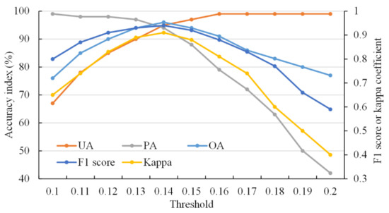
Figure 6.
Classification accuracy for various thresholds based on CFI images derived from Sentinel-2 images on 20 March 2020 in the first study area. UA = user accuracy of canola category, PA = production accuracy of canola category, OA = overall accuracy.
3.5. Classification Results
A map of the canola planting distribution in 2020 was obtained based on the decision tree model classification method, as shown in Figure 7. The canola planting areas were 45.14 km2, 168.93 km2, and 810.36 km2 in the first, second and third study areas, respectively. Canola was distributed mainly in plains or valleys. In the third study area, canola plots were very regular relative to those of the other two study areas.
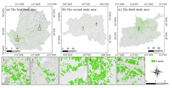
Figure 7.
Distribution of canola planting regions in the three study areas in 2020. (a–c) The canola map in the first, second, and third study area respectively.
The classification accuracy is shown in Table 6. There, the classification results from the decision tree model are compared with those from the SVM classification method. The results show that the classification accuracies of the two classification methods were very similar. The overall accuracy was approximately 96%, with a kappa coefficient of 0.91.

Table 6.
Classification accuracy of CFI images by using the decision tree model, SVM and RF.
Note that when using the decision tree model to identify canola in the second and third study areas, new training samples were not used. However, new training samples were used in the SVM method. That was because when using the SVM method as a classification system, the training samples produced on one image were difficult to apply to another image. In addition, the classification speed of the decision tree model was approximately 60 times that of the SVM method.
Therefore, it was judged that the classification accuracy and robustness of the decision tree model made it appropriate for the automatic identification of canola.
Figure 8 shows the accuracy results of some validation quadrats, which intuitively and visually express the spatial distribution of classification accuracy. Misclassification occurred mainly at the boundary regions of various categories, and some roads less than 10 m wide could not be accurately identified. However, the interiors of the canola plots could usually be accurately identified by using the method proposed in this study.
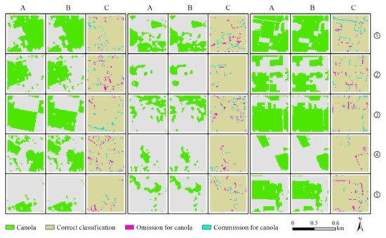
Figure 8.
Results of accuracy validation based on 15 validation quadrats with dimensions of 0.5 km × 0.5 km, selected randomly from 45 validation quadrats. Columns A, B, and C are ground-truth data, classification results, and accuracy results, respectively.
The classification result areas of canola were compared with their ground-truth areas for each validation quadrat, as shown in Figure 9. It demonstrates that the identification areas of canola were very similar to the ground-truth area of canola, with a correlation coefficient of 0.996. Production and user accuracy were also balanced, as shown in Table 6. In other words, the omission rate and commission rate for canola were balanced. Therefore, the identification areas of the canola were very close to the actual areas.
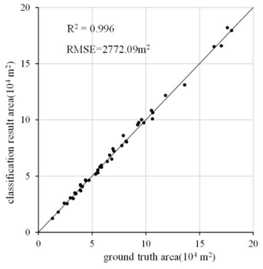
Figure 9.
Canola area scatterplot of validation quadrats from ground-truth surface samples and classification result samples. RMSE denotes the root mean square error.
3.6. Performance of Other Canola Indices
The results of classification accuracy based on various existing canola indices using different methods were plotted in Table 7. No matter which method was used, CFI had the best performance for identifying canola, as shown in Table 7. For CFI, its production accuracy of the canola category was similar to its user accuracy of the canola category, especially when using the SVM and RF methods. This showed that the omission rate of canola and misclassification rate of canola were similar in the classification results based on CFI images. These two errors will offset each other, so that the areas of canola in the classification results are closer to the truth. For overall accuracy and kappa coefficient, the classification accuracy of NDYI was second only to CFI, followed by CI and CRI.

Table 7.
Classification accuracy of different canola indices by using different methods.
In order to more intuitively reflect the classification performances difference between CFI and other indices, we counted the histograms of some objects based on different canola index images derived from Sentinel-2 image on 20 March 2020, as shown in Figure 10.
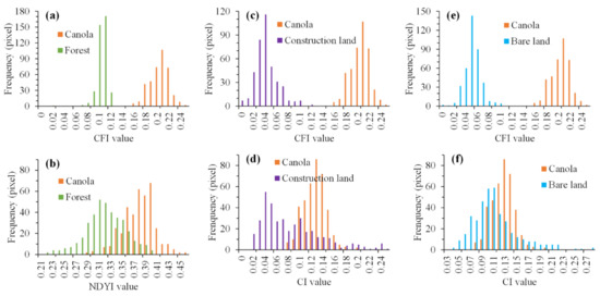
Figure 10.
Histograms of various objects based on various canola flower indices. (a,c,e) Histograms of canola, forest, construction land, and bare land based on CFI values. (b) Histograms of canola and forest based on NDYI values. (d,f) Histogram of canola, construction land, and bare land based on CI values.
NDYI cannot completely distinguish between forest and canola in certain forest areas, while the CFI was better at identifying canola, as shown in Figure 10. Some construction land regions were wrongly identified as canola by using the CI, as shown in Figure 10d. Although the reflectance of construction land in the NIR waveband was less than that of canola, its reflectance in the red and green wavebands was greater than that of canola. Hence, CI ranges of construction land overlapped with canola. Similarly, the CI cannot fully distinguish canola from bare land, as shown in Figure 10f. However, the CFI could fully distinguish canola from construction land and bare land.
4. Discussion
This study developed a novel CFI for automatic canola mapping. The CFI is a spectral index for canola field detection using remote-sensing data. Its advantages are calculation simplicity and effectiveness, and a high automation level.
The spectral difference between canola and winter wheat was slight during their most-growth stages. Wheat can seriously reduce the mapping accuracy of canola, especially in mixed planting areas of wheat and canola. However, the yellow canola flowers provide another opportunity to distinguish between canola and winter wheat, even though the flowering stage is transitory, only about one month [3].
According to our observations, the yellow flowers of canola can create a visual difference between canola fields and winter wheat fields. The most spectral differences between yellow petals and non-yellow petals are visible in the green and red bands [46]. The content of carotenoids in the canola petal is very high; they absorb blue light and reflect green and red light [3]. At the vegetation canopy scale, the recorded spectral reflectance values came from the canola’s yellow flowers and green leaves and stems. The values from other crops, including winter wheat, came only from their green leaves and stems [11,47]. As a result, the spectral reflectance values of canola in the red and green bands were higher than those of other vegetation types during the canola flowering season. However, in the blue and NIR bands, the spectral reflectance values of canola and other vegetation types were similar.
The red-edge bands of Sentinel-2 images play an important role in establishing parameters such as the leaf area index [48]. However, in this study it was not found that the red-edge bands made a significant contribution to the identification of canola according to our previous experimental results. As Griffiths, Nendel and Hostert [32] pointed out, the red-edge bands only slightly improve overall accuracy. In addition, the spatial resolution of the red-edge bands is 20 m × 20 m, which is lower than that of blue, green, red, and NIR bands, whose spatial resolution is 10 m × 10 m. Therefore, the red-edge bands were not used to build the CFI in this study.
The reflectivity of most ground objects in the blue waveband is usually low. Under the influence of a complex atmospheric environment, sometimes the reflectivity of ground objects might be close to zero in the blue band of an atmospheric corrected image. At that time, the NDYI of those objects will be similar to that of canola flowers, even if their reflectivity in the green band is much lower. This phenomenon was found in the Sentinel-2 image on 12 April 2020 in the third study region. Nevertheless, the CFI can effectively avoid similar problems. For example, the NDYI cannot completely distinguish between forest and canola in some particular forest areas, whereas the CFI had better performance at identifying canola, as shown in Figure 10.
During the canola flowering stage, the CFI values of the canola field were greater than the threshold of 0.14, as shown in Figure 11. However, the CFI value of canola did not exceed the threshold in other growth stages. Therefore, the decision tree model based on CFI images can achieve the automatic and accurate identification of canola.
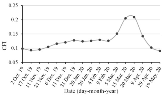
Figure 11.
Time series of canola flower index curve of a canola field during its entire growth cycle.
The flowering period of canola is only approximately 1 mon. Suppose no remote-sensing images were available during the flowering period, due to the influence of cloud and rain. In that case, it would be difficult to identify the planting distribution of canola by using the method proposed in this study. This is the limitation of using optical imagery data to identify canola.
Of course, at the development stage, the automated algorithm requires substantial expert input and image analysis to isolate type-specific properties from inter-annual and inter-region variability [13]. It was concluded that an important research direction is to evaluate the ability of the CFI in different years by considering various climates and other conditions in future research to verify the results of this study.
5. Conclusions
The spectral index, the CFI, proposed in this study, is extremely sensitive to yellow canola flowers. Therefore, the CFI has great potential to identify canola planting distribution accurately. The following conclusions were drawn:
The flowering stage of canola is the best time to identify its planting distribution by remote-sensing data, especially in mixed planting areas of different types of winter crops.
CFI integrates four kinds of spectral information: blue, green, red, and NIR wavebands. It dramatically reduces the dimensions and volume of remote-sensing data and enhances the image information of canola flowers.
The decision tree model based on CFI images can improve the classification accuracy of canola compared to other canola indices. In addition, this decision tree model has good universality. When this model is applied elsewhere, the model threshold does not need to be adjusted.
6. Patents
One Chinese invention patent, an automatic canola identification method based on optical satellite imagery (grant number ZL202010021111.6), resulted from the work reported in this manuscript.
Author Contributions
Conceptualization, H.T. and Y.Q.; methodology, H.T. and T.C.; software, Q.M. and M.Y.; validation, H.T.; formal analysis, H.T. and S.W.; investigation, H.T.; resources, H.T. and Y.Q.; data curation, H.T. and Y.W.; writing—original draft preparation, H.T.; writing—review and editing, Q.L. and Y.Q.; visualization, H.T. and Q.L.; supervision, H.T.; project administration, H.T.; funding acquisition, H.T. and Y.Q. All authors have read and agreed to the published version of the manuscript.
Funding
This research was funded by the Natural Science Foundation of Henan, grant number 202300410075; the China Postdoctoral Science Foundation, grant number 2019M662478; the major project of the Collaborative Innovation Center on Yellow River Civilization, jointly built by the Henan province and the Ministry of Education, grant number 2020M19; and the National Demonstration Center for Experimental Environment and Planning Education (Henan University) Funding Project, grant number 2020HGSYJX009.
Institutional Review Board Statement
Not applicable.
Informed Consent Statement
Not applicable.
Data Availability Statement
https://figshare.com/s/398f0f02a8a9107e34c4 (18 January 2022).
Acknowledgments
We thank the Dabieshan National Observation and Research Field Station of Forest Ecosystem at Henan for its technical assistance.
Conflicts of Interest
The authors declare no conflict of interest.
References
- Sulik, J.J.; Long, D.S. Spectral considerations for modeling yield of canola. Remote Sens. Environ. 2016, 184, 161–174. [Google Scholar] [CrossRef] [Green Version]
- Tian, H.; Meng, M.; Wu, M.; Niu, Z. Mapping spring canola and spring wheat using Radarsat-2 and Landsat-8 images with Google Earth Engine. Curr. Sci. 2019, 116, 291–298. [Google Scholar] [CrossRef]
- Sulik, J.J.; Long, D.S. Spectral indices for yellow canola flowers. Int. J. Remote Sens. 2015, 36, 2751–2765. [Google Scholar] [CrossRef]
- Brown, J.C.; Kastens, J.H.; Victoria, D.D.C.; Bishop, C.R.; Coutinho, A.C. Classifying multiyear agricultural land use data from Mato Grosso using time-series MODIS vegetation index data. Remote Sens. Environ. Interdiscip. J. 2013, 130, 39–50. [Google Scholar] [CrossRef] [Green Version]
- Wang, J.; Wu, C.; Wang, X.; Zhang, X. A new algorithm for the estimation of leaf unfolding date using MODIS data over China’s terrestrial ecosystems. ISPRS J. Photogramm. Remote Sens. 2019, 149, 77–90. [Google Scholar] [CrossRef]
- Tian, H.; Qin, Y.; Niu, Z.; Wang, L.; Ge, S. Summer Maize Mapping by Compositing Time Series Sentinel-1A Imagery Based on Crop Growth Cycles. J. Indian Soc. Remote Sens. 2021, 49, 2863–2874. [Google Scholar] [CrossRef]
- Arango, R.B.; Campos, A.M.; Combarro, E.F.; Canas, E.R.; Diaz, I. Mapping cultivable land from satellite imagery with clustering algorithms. Int. J. Appl. Earth Obs. Geoinf. 2016, 49, 99–106. [Google Scholar] [CrossRef]
- Yariyan, P.; Janizadeh, S.; Van Tran, P.; Nguyen, H.D.; Costache, R.; Van Le, H.; Pham, B.T.; Pradhan, B.; Tiefenbacher, J.P. Improvement of Best First Decision Trees Using Bagging and Dagging Ensembles for Flood Probability Mapping. Water Resour. Manag. 2020, 34, 3037–3053. [Google Scholar] [CrossRef]
- Vaudour, E.; Noirot-Cosson, P.E.; Membrive, O. Early-season mapping of crops and cultural operations using very high spatial resolution Pleiades images. Int. J. Appl. Earth Obs. Geoinf. 2015, 42, 128–141. [Google Scholar] [CrossRef]
- Tian, H.F.; Pei, J.; Huang, J.X.; Li, X.C.; Wang, J.; Zhou, B.Y.; Qin, Y.C.; Wang, L. Garlic and Winter Wheat Identification Based on Active and Passive Satellite Imagery and the Google Earth Engine in Northern China. Remote Sens. 2020, 12, 3539. [Google Scholar] [CrossRef]
- Ashourloo, D.; Shahrabi, H.S.; Azadbakht, M.; Aghighi, H.; Nematollahi, H.; Alimohammadi, A.; Matkan, A.A. Automatic canola mapping using time series of sentinel 2 images. ISPRS J. Photogramm. Remote Sens. 2019, 156, 63–76. [Google Scholar] [CrossRef]
- Foerster, S.; Kaden, K.; Foerster, M.; Itzerott, S. Crop type mapping using spectral-temporal profiles and phenological information. Comput. Electron. Agric. 2012, 89, 30–40. [Google Scholar] [CrossRef] [Green Version]
- Zhong, L.H.; Hu, L.N.; Yu, L.; Gong, P.; Biging, G.S. Automated mapping of soybean and corn using phenology. ISPRS J. Photogramm. Remote Sens. 2016, 119, 151–164. [Google Scholar] [CrossRef] [Green Version]
- Tian, H.; Huang, N.; Niu, Z.; Qin, Y.; Pei, J.; Wang, J. Mapping Winter Crops in China with Multi-Source Satellite Imagery and Phenology-Based Algorithm. Remote Sens. 2019, 11, 820. [Google Scholar] [CrossRef] [Green Version]
- Pan, L.; Xia, H.; Yang, J.; Niu, W.; Wang, R.; Song, H.; Guo, Y.; Qin, Y. Mapping cropping intensity in Huaihe basin using phenology algorithm, all Sentinel-2 and Landsat images in Google Earth Engine. Int. J. Appl. Earth Obs. Geoinf. 2021, 102, 102376. [Google Scholar] [CrossRef]
- Pan, L.; Xia, H.M.; Zhao, X.Y.; Guo, Y.; Qin, Y.C. Mapping Winter Crops Using a Phenology Algorithm, Time-Series Sentinel-2 and Landsat-7/8 Images, and Google Earth Engine. Remote Sens. 2021, 13, 2510. [Google Scholar] [CrossRef]
- Tian, H.; Wang, Y.; Chen, T.; Zhang, L.; Qin, Y. Early-Season Mapping of Winter Crops Using Sentinel-2 Optical Imagery. Remote Sens. 2021, 13I, 3822. [Google Scholar] [CrossRef]
- Zhang, G.; Xiao, X.; Dong, J.; Kou, W.; Jin, C.; Qin, Y.; Zhou, Y.; Wang, J.; Menarguez, M.A.; Biradar, C. Mapping paddy rice planting areas through time series analysis of MODIS land surface temperature and vegetation index data. ISPRS J. Photogramm. Remote Sens. 2015, 106, 157–171. [Google Scholar] [CrossRef] [Green Version]
- Tang, K.; Zhu, W.Q.; Zhan, P.; Ding, S.Y. An Identification Method for Spring Maize in Northeast China Based on Spectral and Phenological Features. Remote Sens. 2018, 10, 193. [Google Scholar] [CrossRef] [Green Version]
- d’Andrimont, R.; Taymans, M.; Lemoine, G.; Ceglar, A.; Yordanov, M.; van der Velde, M. Detecting flowering phenology in oil seed rape parcels with Sentinel-1 and-2 time series. Remote Sens. Environ. 2020, 239, 111660. [Google Scholar] [CrossRef]
- Mercier, A.; Betbeder, J.; Baudry, J.; Le Roux, V.; Spicher, F.; Lacoux, J.; Roger, D.; Hubert-Moy, L. Evaluation of Sentinel-1 & 2 time series for predicting wheat and rapeseed phenological stages. ISPRS J. Photogramm. Remote Sens. 2020, 163, 231–256. [Google Scholar] [CrossRef]
- Tao, J.-B.; Liu, W.-B.; Tan, W.-X.; Kong, X.-B.; Xu, M. Fusing multi-source data to map spatio-temporal dynamics of winter rape on the Jianghan Plain and Dongting Lake Plain, China. J. Integr. Agric. 2019, 18, 2393–2407. [Google Scholar] [CrossRef]
- Han, J.; Zhang, Z.; Luo, Y.; Cao, J.; Li, Z. The RapeseedMap10 database: Annual maps of rapeseed at a spatial resolution of 10 m based on multi-source data. Earth Syst. Sci. Data 2021, 13, 2857–2874. [Google Scholar] [CrossRef]
- Zang, Y.; Chen, X.; Chen, J.; Tian, Y.; Cui, X. Remote Sensing Index for Mapping Canola Flowers Using MODIS Data. Remote Sens. 2020, 12, 3912. [Google Scholar] [CrossRef]
- Fang, S.H.; Tang, W.C.; Peng, Y.; Gong, Y.; Dai, C.; Chai, R.H.; Liu, K. Remote Estimation of Vegetation Fraction and Flower Fraction in Oilseed Rape with Unmanned Aerial Vehicle Data. Remote Sens. 2016, 8, 416. [Google Scholar] [CrossRef] [Green Version]
- Pta, B.; Pst, A.; Ao, A.; Jx, B.; Mkg, C.; Rgc, D.; Ky, D.; Ah, E. A 30-m landsat-derived cropland extent product of Australia and China using random forest machine learning algorithm on Google Earth Engine cloud computing platform. ISPRS J. Photogramm. Remote Sens. 2018, 144, 325–340. [Google Scholar]
- Guo, Y.; Xia, H.; Pan, L.; Zhao, X.; Li, R. Mapping the Northern Limit of Double Cropping Using a Phenology-Based Algorithm and Google Earth Engine. Remote Sens. 2022, 14, 1004. [Google Scholar] [CrossRef]
- Yi-Tong, L.; Jun, W. Application of HJ-1A/B-CCD Images in Extracting the Distribution of Winter Wheat and Rape in Hubei Province. Chin. J. Agrometeorol. 2012, 33, 573–578. [Google Scholar]
- Drusch, M.; Bello, U.D.; Carlier, S.; Colin, O.; Fernandez, V.; Gascon, F.; Hoersch, B.; Isola, C.; Laberinti, P.; Martimort, P.; et al. Sentinel-2: ESA’s Optical High-Resolution Mission for GMES Operational Services. Remote Sens. Environ. 2012, 120, 25–36. [Google Scholar] [CrossRef]
- Labib, S.M.; Harris, A. The potentials of Sentinel-2 and LandSat-8 data in green infrastructure extraction, using object based image analysis (OBIA) method. Eur. J. Remote Sens. 2018, 51, 231–240. [Google Scholar] [CrossRef]
- Zheng, Y.; Wu, B.; Zhang, M. Estimating the above ground biomass of winter wheat using the Sentinel-2 data. J. Remote Sens 2017, 21, 318–328. [Google Scholar]
- Griffiths, P.; Nendel, C.; Hostert, P. Intra-annual reflectance composites from Sentinel-2 and Landsat for national-scale crop and land cover mapping. Remote Sens. Environ. 2019, 220, 135–151. [Google Scholar] [CrossRef]
- Amani, M.; Ghorbanian, A.; Ahmadi, S.A.; Kakooei, M.; Brisco, B. Google Earth Engine Cloud Computing Platform for Remote Sensing Big Data Applications: A Comprehensive Review. IEEE J. Sel. Top. Appl. Earth Obs. Remote Sens. 2020, 13, 5326–5350. [Google Scholar] [CrossRef]
- Gorelick, N.; Hancher, M.; Dixon, M.; Ilyushchenko, S.; Thau, D.; Moore, R. Google Earth Engine: Planetary-scale geospatial analysis for everyone. Remote Sens. Environ. 2017, 202, 18–27. [Google Scholar] [CrossRef]
- Fensholt, R.; Proud, S.R. Evaluation of Earth Observation based global long term vegetation trends—Comparing GIMMS and MODIS global NDVI time series. Remote Sens. Environ. 2012, 119, 131–147. [Google Scholar] [CrossRef]
- Zheng, K.; Wei, J.Z.; Pei, J.Y.; Cheng, H.; Zhang, X.L.; Huang, F.Q.; Li, F.M.; Ye, J.S. Impacts of climate change and human activities on grassland vegetation variation in the Chinese Loess Plateau. Sci. Total Environ. 2019, 660, 236–244. [Google Scholar] [CrossRef]
- Tian, H.; Wu, M.; Wang, L.; Niu, Z. Mapping Early, Middle and Late Rice Extent Using Sentinel-1A and Landsat-8 Data in the Poyang Lake Plain, China. Sensors 2018, 18, 185. [Google Scholar] [CrossRef] [Green Version]
- Verma, A.K.; Garg, P.K.; Prasad, K.S.H. Sugarcane crop identification from LISS IV data using ISODATA, MLC, and indices based decision tree approach. Arab. J. Geosci. 2017, 10, 16. [Google Scholar] [CrossRef]
- Bazi, Y.; Melgani, F. Toward an optimal SVM classification system for hyperspectral remote sensing images. IEEE Trans. Geosci. Remote Sens. 2006, 44, 3374–3385. [Google Scholar] [CrossRef]
- Koda, S.; Zeggada, A.; Melgani, F.; Nishii, R. Spatial and Structured SVM for Multilabel Image Classification. IEEE Trans. Geosci. Remote Sens. 2018, 56, 5948–5960. [Google Scholar] [CrossRef]
- Breiman, L. Random forests. Mach. Learn. 2001, 45, 5–32. [Google Scholar] [CrossRef] [Green Version]
- Min, X.; Watanachaturaporn, P.; Varshney, P.K.; Arora, M.K. Decision tree regression for soft classification of remote sensing data. Remote Sens. Environ. 2005, 97, 322–336. [Google Scholar]
- Card, D.H. Using known map category marginal frequencies to improve estimates of thematic map accuracy. Photogramm. Eng. Remote Sens. 1982, 48, 431–439. [Google Scholar]
- Olofsson, P.; Foody, G.M.; Stehman, S.V.; Woodcock, C.E. Making better use of accuracy data in land change studies: Estimating accuracy and area and quantifying uncertainty using stratified estimation. Remote Sens. Environ. 2013, 129, 122–131. [Google Scholar] [CrossRef]
- Hripcsak, G.; Rothschild, A.S. Agreement, the F-measure, and reliability in information retrieval. J. Am. Med. Inform. Assoc. 2005, 12, 296–298. [Google Scholar] [CrossRef]
- Yates, D.J.; Steven, M.D. Reflexion and absorption of solar radiation by flowering canopies of oil-seed rape (Brassica napus L.). J. Agric. Sci. 1987, 109, 495–502. [Google Scholar] [CrossRef]
- Wilson, J.H.; Zhang, C.H.; Kovacs, J.M. Separating Crop Species in Northeastern Ontario Using Hyperspectral Data. Remote Sens. 2014, 6, 925–945. [Google Scholar] [CrossRef] [Green Version]
- Clevers, J.G.P.W.; Kooistra, L.; van den Brande, M.M.M. Using Sentinel-2 Data for Retrieving LAI and Leaf and Canopy Chlorophyll Content of a Potato Crop. Remote Sens. 2017, 9, 405. [Google Scholar] [CrossRef] [Green Version]
Publisher’s Note: MDPI stays neutral with regard to jurisdictional claims in published maps and institutional affiliations. |
© 2022 by the authors. Licensee MDPI, Basel, Switzerland. This article is an open access article distributed under the terms and conditions of the Creative Commons Attribution (CC BY) license (https://creativecommons.org/licenses/by/4.0/).