Article

Verification and Validation of Hybridspectral Radiometry Obtained from an Unmanned Surface Vessel (USV) in the Open and Coastal Oceans

by
Stanford B. Hooker
1,*,†,
Henry F. Houskeeper
2,†,
Randall N. Lind
3,
Raphael M. Kudela
4 and
Koji Suzuki
5
1
NASA Goddard Space Flight Center, Greenbelt, MD 20771, USA
2
Department of Geography, University of California, Los Angeles, CA 90095, USA
3
Biospherical Instruments Inc., San Diego, CA 92110, USA
4
Ocean Sciences Department, University of California, Santa Cruz, CA 95064, USA
5
Faculty of Environmental Earth Science, Hokkaido University, Sapporo 060-0810, Japan
*
Author to whom correspondence should be addressed.
These authors contributed equally to this work.
Remote Sens. 2022, 14(5), 1084; https://doi.org/10.3390/rs14051084
Submission received: 19 January 2022 / Revised: 8 February 2022 / Accepted: 12 February 2022 / Published: 23 February 2022

Abstract

:
The hardware and software capabilities of the compact-profiling hybrid instrumentation for radiometry and ecology (C-PHIRE) instruments on an unmanned surface vessel (USV) are evaluated. Both the radiometers and USV are commercial-off-the-shelf (COTS) products, with the latter being only minimally modified to deploy the C-PHIRE instruments. The hybridspectral C-PHIRE instruments consist of an array of 18 multispectral microradiometers with 10 nm wavebands spanning 320–875 nm plus a hyperspectral compact grating spectrometer (CGS) with 2048 pixels spanning 190–1000 nm. The C-PHIRE data were acquired and processed using two architecturally linked software packages, thereby allowing lessons learned in one to be applied to the other. Using standard data products and unbiased statistics, the C-PHIRE data were validated with those from the well-established compact-optical profiling system (C-OPS) and verified with the marine optical buoy (MOBY). Agreement between algorithm variables used to estimate colored dissolved organic matter (CDOM) absorption and chlorophyll a concentration were also validated. Developing and operating novel technologies, such as the C-PHIRE series of instruments, deployed on a USV increase the frequency and coverage of optical observations, which are required to fully support the present and next-generation validation exercises in radiometric remote sensing of aquatic ecosystems.

1. Introduction

As ocean-observing satellites age, replacements are a critical requirement to maintain a quality assured time series of planetary climate [1], typically referred to as a climate data record (CDR). The continuity of CDRs from legacy Earth observation system (EOS) missions [2] and beyond is an international activity shared between space agencies launching new satellites and researchers who vicariously calibrate the spaceborne radiances, subsequently validating the algorithms used to derive data products, and pursue original research. This calibration, validation, and research (CVR) triad determines mission success and establishes the requirements for follow-on missions. The spatial and temporal scales involved are typically the most restrictive for calibration observations and expand throughout validation and research inquiries for each mission with the latter typically justifying the principal science objectives for new missions [3].
Dedicated field data for CVR activities are acquired throughout an ocean color satellite mission in accordance with long-standing requirements in the NASA Ocean Optics Protocols [4,5,6,7,8], hereafter referred to as the Protocols. Although the Protocols include differences within the CVR triad, e.g., allowed water masses or permissible uncertainties, the underlying core requirements for optical measurements are basically the same [9]. The core similarities allow the opportunity for CVR data acquisition to be accomplished with a single platform design, although it is acknowledged that the extremely small scale of inland waters, e.g., a narrow shallow river or extremely turbid lake, ultimately requires unique designs defying a common architecture for all water bodies. The exclusion of the most restrictive waters account for less than 1% of aquatic surface waters and do not contribute significantly to the dynamic range of the log-normal bio-optical variables typically used in optical oceanographic research [10], so their exclusion does not degrade the potential global applicability of the approach presented here to more than 99% of the aquatic surface area.
The common deployment architecture considered herein is based on an unmanned surface vessel (USV) that can be deployed within the near-surface waters of open and coastal oceans, marginal seas, plus the largest inland water bodies, of which there are more than 30 [11]. The remote sensing observations from the USV presented herein span the majority of the dynamic range in global aquatic total chlorophyll a concentration, C a , and were obtained in open and coastal oceans off Hawaii (oligotrophic), Puerto Rico (mesotrophic), and California (eutrophic). Observations from the latter include remote characterization of a harmful algal bloom (HAB). An inland California reservoir (eutrophic) was also sampled to allow for trials associated with alternative software configurations of the CGS. The dynamic range is confirmed by independent shipborne sampling and subsequent laboratory analyses of the water masses transited by the USV. The shipborne sampling also includes validation of the remote sensing radiometry on the USV using a separate in-water profiler.
As part of validating instrument performance and establishing operational readiness of the remote sensing system that was developed, the results presented are applicable to all three activities within the CVR triad. Vicarious calibration, which is a system-level process accounting for atmospheric correction biases and prelaunch calibration changes resulting from placing a radiometer in orbit, is arguably the most exacting, so a succinct summary of the distinguishing aspects beyond standard practice are as follows:
C1
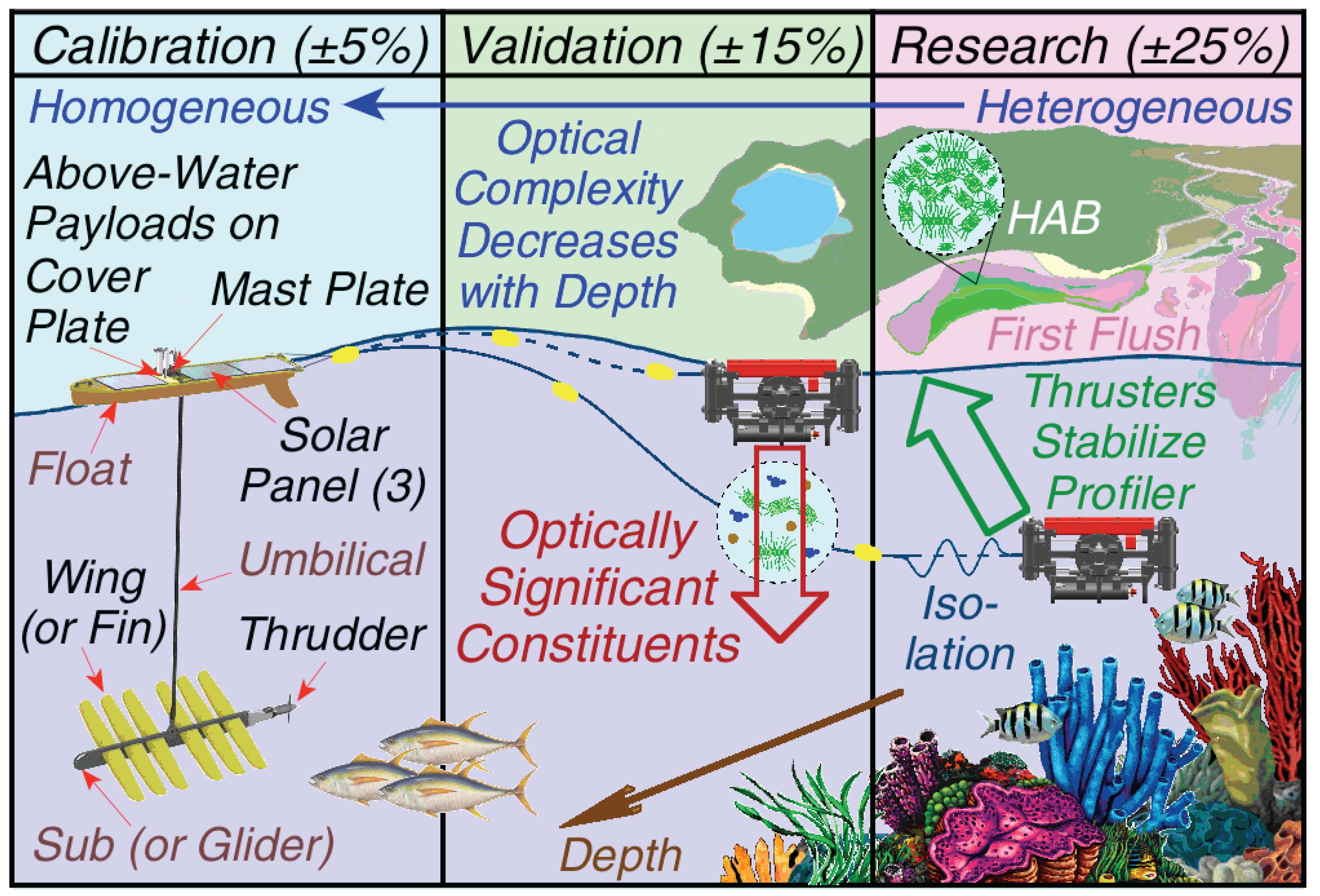
Data are obtained within exceptionally clear waters with horizontally homogeneous optical properties (over several kilometers and typically in the deep ocean);
C2
Properly characterized hyperspectral instruments, calibrated with radiometric traceability to the National Institute of Standards and Technology (NIST), are used so spectral response functions for the satellite instrument can be applied; and
C3
Sampling is under clear skies, stable illumination, and marine aerosols (verified with shadow band or sun photometer data) with extraordinary calibration maintenance.
Historically, this activity has used a dedicated platform moored in deep oceanic water and hosting custom-built hyperspectral radiometers to measure apparent optical properties (AOPs), e.g., the Marine Optical Buoy (MOBY) activity [12]. The Bouée pour l’acquisition de Séries Optiques à Long Terme (BOUSSOLE) mooring, however, initially used commercial-off-the-shelf (COTS) multispectral radiometers and fulfilled CDR requirements for legacy satellite instruments [13].
The additional activities of the CVR triad are less exacting, but must span a greater temporal and spatial extent to support the validation and research objectives of the community. Remote sensing using autonomous in-water profilers is a cost-efficient approach to greatly increase the availability of bio-optical data products, and examples of low-cost activities intended to support the research component of the CVR triad are increasing, e.g., deploying bio-optical sensors on an Argo float [14]. Developing mature technologies that increase the frequency and coverage of validation-quality aquatic observations is required to support present and next-generation validation activities including the phytoplankton, aerosol, cloud, ocean ecosystem (PACE) mission.
The hybridspectral alternative for remote profiling of optical observations for NASA satellites (HARPOONS) activity combined the following COTS technological advances: (a) digital thrusters to obtain a vertical profile of AOPs [15]; (b) use of a USV that can be launched from a small boat as the remote sensing platform (rather than a deep-sea mooring) to simplify deployments, reduce costs, and mitigate vandalism [16]; and (c) a hyperspectral capability with companion multispectral detectors [17], which is referred to as hybridspectral. The autonomous capability allows for rapid mission reassignment to span global sampling within the CVR triad. All detectors operate simultaneously, but the multispectral detectors have 10 decades of dynamic range and sample at 15 Hz, thereby allowing a unique validation opportunity for the spectrally more expansive—but potentially less responsive and slower—spectrographs, depending on wavelength and environmental conditions. The objective of this study is to evaluate the efficacy of the hardware and software deployed as part of the HARPOONS activity to define appropriate future remote sensing applications for the underlying autonomous technologies.

2. Materials and Methods

The common deployment architecture is based on a COTS USV towing an optical package that obtains a near-surface vertical profile of AOPs while simultaneously obtaining above-water AOPs. The latter permits the derivation of normalized data products to account for changes in solar illumination during optical data acquisition or comparison. The USV follows a predetermined set of sequential waypoints, but can also respond to remote operator commands. An onboard computer located in a payload dry box controls all instruments and acquires all data. The computer can be controlled (i.e., reconfigured) at sea through a wireless fidelity (WiFi) connection established on a small boat in near proximity to the USV. The occasional visits by the small boat fulfill two important functions, as follows: (a) independent AOP observations to verify and validate the data products produced from the USV instruments; and (b) collection of seawater samples for laboratory analyses to validate the dynamic range of constituents and the use of any algorithms applied to the USV data products. The principal water mass constituents are C a plus the colored (or chromophoric, depending on the literature) dissolved organic matter (CDOM) spectral absorption coefficient, a CDOM ( λ ) , with specific application to a CDOM ( 440 ) .

2.1. COTS USV

The USV selected for this study was a third-generation surface vessel, or SV3, developed by Liquid Robotics, Inc. (LRI) as part of the COTS Wave Glider series they manufacture (Sunnyvale, CA, USA). The three principal subsystems of an SV3 are a buoyant hull or float, a submerged glider or sub, plus a cable assembly or umbilical connecting the two to create a single electromechanical system suitable for CVR activities (Figure 1). The addition of above- and in-water optical instruments with needed ancillary sensors creates an autonomous remote sensing platform to support CVR activities. Above-water optical instruments are mounted on the SV3 cover plate, communications are mounted on the mast plate, support electronics (including batteries) are contained within dry boxes under the three solar panels, and in-water optical instruments are mounted on a backplane with profiling thrusters that are towed using a two-point harness attached to a 30–35 m sea cable routed through the stern of the float. To optimize the quality of the optical data, the SV3 is launched for a 10 d mission during clear skies and fair weather (no severe weather forecasted). The payload includes additional rechargeable batteries to allow for the failure of a solar panel without compromising mission fidelity.
The float rides on the surface of the water and typically contains the following: (a) one or more battery modules charged by three solar panels; (b) command and control unit (CCU) electronics with a GPS antenna and bulkhead connections for optional payloads; (c) a mast plate with side and center lift points; (d) a neighboring cover plate for attaching optional payloads; (e) a global positioning system (GPS) tracker; and (f) rear stabilizing handles. The CCU typically also supports a weather station, an automatic identification system (AIS) receiver, which is used for collision avoidance, plus long-(satellite) and short-range communications, e.g., cellular, which are mounted on the mast plate. Both medium- and large-sized vessels most capable of damaging the SV3 are required to have AIS. The tracker provides SV3 location at a coarser temporal resolution (user selected based on independent internal battery constraints) and continues to function if the float is flipped upside down.
The sub is positioned at a nominal depth, established by the length of the umbilical (4 m), and is comprised of a set of wings (or fins), one or more payloads, and a thruster–rudder combination known as a thrudder (thrudder propulsion was not used in this study). The propulsion mechanism is based on harvesting the wave energy difference between the float and the sub to create forward thrust. A rising wave lifts the float, which raises the sub. The articulated wings on the sub press down to create an up-and-forward motion, in turn pulling the float forward and off the wave. This causes the sub to drop and the wings to pivot up, and the sub moves down and forward. This up-and-down synchronization results in an irregular, but consistently forward, motion that is repeated as long as there are waves on the surface, even when their amplitude is rather small.
The umbilical is a streamlined connector with high-strength components to support the weight of the sub and the tension the float and sub exert on each other in response to wave motion. The umbilical contains wiring to access the float power system, control the thruster and rudder capabilities of the thrudder, and communicate with any scientific payloads. The thrudder can be used to increase the rate of forward progress of the SV3, e.g., to maneuver more quickly away from collision threats identified by the AIS system, albeit at the expense of higher power consumption.
Wave gliders were used successfully to tow payloads from the sub unit [18], but this limits the amount of power to the towed payload based on the number of conductors and wire gauges in the umbilical. The umbilical is connected to the wave glider power system, which provides power more similar to a power supply than a battery, wherein instantaneous loads, e.g., from (thruster) motors, are sometimes problematic. Because of limitations with power supplied through the umbilical, the towable optical wave-following in situ hybrid (TOW-FISH) profiler was designed and built to be towed from the float. Modifications to the COTS SV3 to allow towing from the float and to accommodate other aspects of the scientific payloads were relatively minor and are provided in summary detail below (Section 2.3).

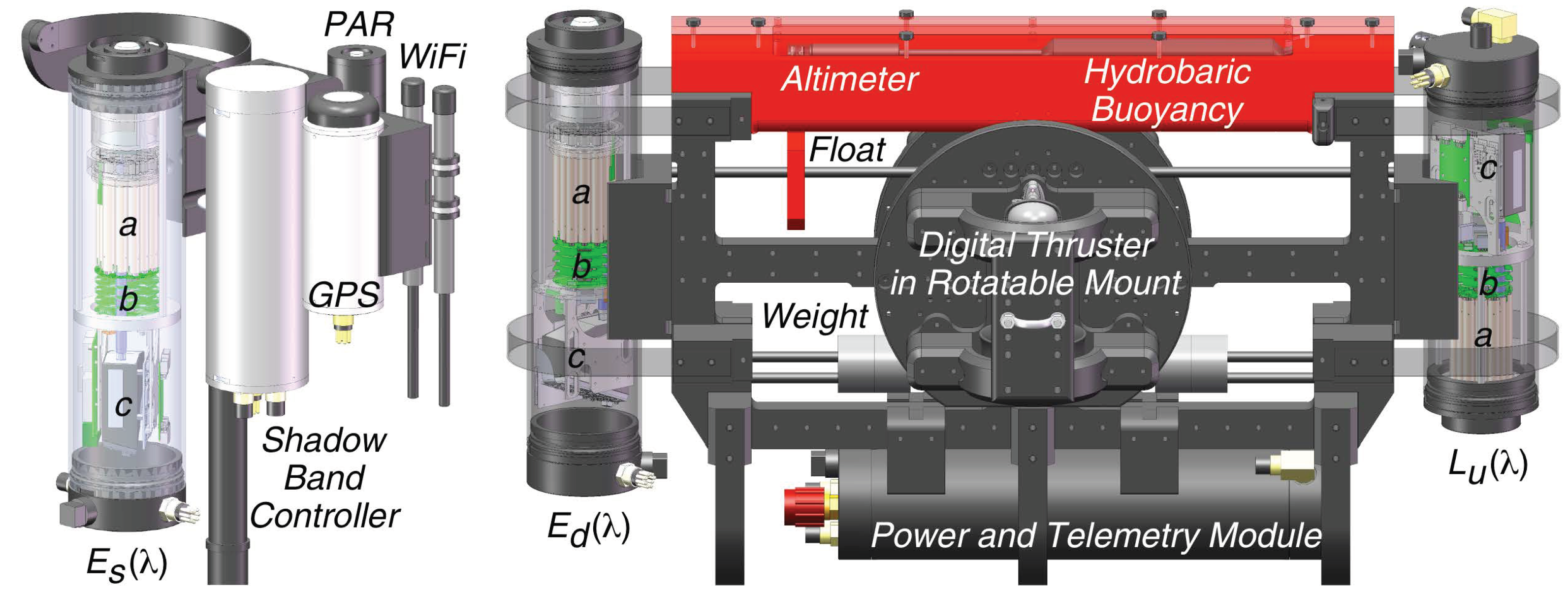
2.2. Optical Observations

An above-water instrument suite was mounted on the float cover plate and was comprised of the following: (a) a global solar irradiance ( E s ), an above-water radiometer equipped with a shadow band accessory to estimate the indirect or diffuse irradiance ( E i ), which improves the self-shading correction for downward-pointing radiometers from in-water observations; (b) a single-channel photosynthetically available radiation (PAR) sensor; (c) a GPS sensor; and (d) dual WiFi antennas. The tallest components are the solar reference and PAR sensor diffusers, which are also taller than the components mounted on the mast plate. In-water radiometers were mounted on the TOW-FISH, which was a modified compact-optical profiling system (C-OPS) backplane [19] with hydrobaric and adjustable buoyancy control plus dual thrusters developed for the compact-propulsion option for profiling systems (C-PrOPS) accessory [15]. The TOW-FISH had downward irradiance ( E d ) and upwelling radiance ( L u ) in-water radiometers and was towed 30–35 m behind the float to ensure shading from the latter was negligible. The sea cable had internal and external strength members, a combination of hydrobaric and fixed buoyancy devices to tune cable drag and set the resting depth, plus an accordion-like isolation section to remove the back-and-forth motions imparted to the sea cable from the motions of the float and sub in the surface wave field.
The E s , E d , and L u radiometers were from the compact-profiling hybrid instrumentation for radiometry and ecology (C-PHIRE) series of instruments. Detailed descriptions of C-PHIRE radiometers are provided by [16,17], so only pertinent summaries are provided herein. C-PHIRE radiometers are hybridspectral and consist of a cluster of multispectral microradiometers [20] with 10 nm wavebands spanning 320–875 nm that acquire data simultaneously with a hyperspectral compact grating spectrometer (CGS) with 2048 pixels spanning 190–1000 nm. Optical data products from the former match the wavebands and from the latter span 290–900 nm and include multispectral bandpass conversions. A microradiometer has a silicon photodetector (SiP) and is manufactured by Biospherical Instruments Inc. (San Diego, CA, USA). The CGS is manufactured by Carl Zeiss Spectroscopy GmbH (Jena, Germany) with tec5USA, Inc. (Plainview, NY, USA) supplying the electronics interface. For the multispectral radiometers, the generalized spectral domains (with wavebands) were as follows: UV (320, 340, 380, and 395 nm); Blue (412, 443, and 490 nm); Green (510, 532, 555, and 589 nm); Red (625, 670, and 683 nm); and NIR (710, 780, 820, and 875 nm). The multispectral coverage, as well as the hyperspectral coverage, exceeds the requirements for next-generation satellite missions in the UV domain [3].
The backplane also contains a pressure transducer to determine depth (z), external water temperature sensor, and high-precision altimeter plus gyro for estimating the geometry of the optical apertures with respect to the sun. The altimeter provides improved depth accuracy and precision close to the sea surface to resolve low-excursion pressure changes in the near-surface optical data [15] and rate gyros remove the effects of wave-driven accelerations [16]. Although tunable, for this study the TOW-FISH had a resting depth of approximately 5–6 m and was scheduled to make a vertical ascent using the two thrusters every 30 min during approximately 1000–1700 local time and then to free-fall back to the stowed depth. Data were acquired from all instruments during the up and down “casts” of the profiler. Shadow band data were obtained after the down cast, and dark data were obtained at night. The PAR sensor was used to confirm nighttime flux levels were suitable for acquiring dark data and to independently confirm atmospheric, as well as illumination, stability. An overview of the above- and in-water instrument suite is shown in Figure 2.
The in-water perspective requires L u ( λ ) observations as a function of depth, z, either at discrete depths or as a vertical profile, with the latter providing the maximum degrees of freedom for deriving data products. Simultaneous in-water downward irradiance, E d ( z , λ ) , and global solar irradiance, E s ( λ ) , measured above the surface z = 0 + are used to set and confirm the extent of the extrapolation interval z 1 and z 2 in a near-surface layer with homogeneous properties. The confirmation process uses a boundary constraint to converge two independent measurements: (a) E d ( z , λ ) extrapolated from within z 1 and z 2 to null depth, 0 , and denoted E d ( 0 , λ ) ; plus (b) E s ( λ ) transmitted through the surface to null depth, and denoted E s ( 0 , λ ) . The convergence process is based on altering z 1 and z 2 —while maintaining the observations are within a homogeneous layer—until the two independent null depth irradiance measurements agree to within 5%. A 5% agreement is close to the calibration uncertainty range of 2.8–3.6% for C-PHIRE SiP and CGS detectors [16] and provides an extrapolation through the central tendency of the in-water light field thereby mitigating wave-focusing effects [21].

2.3. Modifications to the Standard SV3 Configuration

The modifications to the standard SV3 configuration to support the sampling shown in Figure 1 and Figure 2 were as follows:
  • The original cover plate was replaced with a strengthened version of the same dimension to allow the mounting of the above-water instrument suite described in Section 2.2;
  • The cellular and AIS antennas plus the weather station mast were shortened to achieve a final height below the E s ( λ ) and PAR diffusers. Although all shortened components functioned as anticipated, the original AIS unit was subsequently replaced with a model made by Antcom (Torrance, CA, USA), the supplier of the cellular antenna, to ensure height compliance with no alterations to the original device (because AIS functionality is a critical safety requirement);
  • Hard anodized aluminum brackets were added to the stern port and starboard stabilizing handle mounts to support the harness cabling attached to the sea cable used for towing the TOW-FISH with no loss in functionality of the handles;
  • Stainless steel and insulated P-clips plus reinforcing metal plates were used together with longer screws securing the two aft solar panels to allow the sea cable to be held down along the edge of the solar panels without shading the panels;
  • The center pick point on the mast plate was ultimately replaced with an extended pick-point assembly to facilitate SV3 recovery. The original center pick point was positioned rather low and close to the float deck, which was considered somewhat problematic due to the near proximity of the higher above-water instrument suite mounted on the cover plate.

2.4. Optical Data Products

In addition to the null depth data products L u ( 0 , λ ) and E d ( 0 , λ ) , the slope of the linear fit of the corresponding in-water optical data within the extrapolation interval are used to provide unbiased estimates of the corresponding diffuse attenuation coefficients, K L u ( λ ) and K d ( λ ) , respectively. Both K L u ( λ ) and K d ( λ ) are directly tied to the L u ( 0 , λ ) and E d ( 0 , λ ) derived data products, respectively. The water-leaving radiance, L W ( λ ) , is derived from L u ( 0 , λ ) based on the simplistic formulation L W ( λ ) = 0.54 L u ( 0 , λ ) , wherein the 0.54 constant accurately transmits L u ( 0 , λ ) through the sea surface [22]. Normalized L W ( λ ) forms use E s ( λ ) data to allow measurements at different illuminations or times in the same water mass to be compared. For example, the remote sensing reflectance is computed as R rs ( λ ) = L W ( λ ) / E s ( λ ) and a correction for the change in the Earth–Sun distance results in the normalized water-leaving radiance, L W ( λ ) N , which is considered below.
For satellite (or airborne) comparisons, differences in viewing angles and solar geometry are important, so a more complete normalization is required. For case-1 waters [23] wherein C a solely determines the absorption and scattering processes, it is possible to transform the derivation of the in-water L W ( λ ) N into an exact form properly adjusted to remove bidirectional effects, as follows (after removing some of the explicit and implicit dependencies, e.g., aerosol loading on the solar irradiance, and not presenting the equivalent reflectance formulation for brevity):
L W ( λ ) N ex = F ¯ 0 ( λ , t SDY ) N 2 Earth Sun Correction 0.54 L u ( 0 , λ , θ s ) N 1 R rs = der g ( L u , E d , E s ) E s ( λ , θ s ) f 0 ( λ , C a ) Q 0 ( λ , C a ) f ( λ , θ s , C a ) Q n ( λ , θ s , C a ) 1 N 3 f = def g ( E u , E d ) and Q = def g ( E u , L u ) ,
where “ex” denotes the exact form and the under and over braces identify normalization terms (N1–N3). The latter are clarified, as follows:
N1
R rs ( λ ) is derived ( = der ) as a function (denoted g) of L u extrapolated to null depth ( z = 0 ), E d to also define the extrapolation interval, and applicable corrections, e.g., dark currents, aperture offsets, E s temporal (solar transit) changes, self-shading, etc;
N2
The correction for the hypothetical water-leaving radiance that would be measured in the absence of any atmospheric loss with a zenith Sun at the mean Earth–Sun distance is accomplished by adjusting R rs ( λ ) with the time-dependent mean extraterrestrial solar irradiance, F ¯ 0 , which is usually formulated to depend on the sequential day of the year (SDY), t SDY , and is derived from look-up tables [24];
N3
The f term is defined ( = def ) as a function relating the irradiance reflectance ( R = E u / E d ) to the inherent optical properties (IOPs), the bidirectional Q-factor is defined ( = def ) by E u and L u , i.e., Q = E u / L u , wherein f 0 and Q 0 are defined for a zero solar zenith angle ( θ s = 0 ) with nadir viewing at null depth ( Q n ) for the latter, and look-up tables for both are based on the viewing and solar geometry plus the C a .
The C-PHIRE calibration data products were created by the manufacturer. MOBY data were obtained from a large bio-optical archive established at the start of the sea-viewing wide field-of-view sensor (SeaWiFS) satellite mission [1]. The repository is called the SeaWiFS bio-optical archive and storage system (SeaBASS) and is described by [25,26]. All other data were acquired using data acquisition and control for photometric and radiometric observations (DACPRO) software with data products derived using processing of radiometric observations of seawater using information technologies (PROSIT) software, both of which strictly adhere to the Protocols as explained by [16]. Data products for the hyperspectral and multispectral detectors spanned 290–900 nm and 320–875 nm, respectively. A unique feature of the two software packages is they are architecturally linked, so lessons learned in one can be applied to the other.
After calibration, the next simplest data products involve lower-level parameters derived from the in situ observations to begin calculating higher-order variables. For the in-water TOW-FISH, the relevant variables are produced as part of determining the extrapolation interval from which E d ( 0 , λ ) and L u ( 0 , λ ) are derived. The value of E s ( λ ) temporally corresponding to the extrapolation interval time period is also derived. These three variables are the lower-level data products considered herein. The use of the “lower-level” vocabulary should not be construed to suggest the variables are not derived from sophisticated data processing. The PROSIT software includes a preprocessing step that implements a substantive inventory of corrections based on laboratory and field characterizations before determination of the extrapolation interval is attempted. The DACPRO software ensures the needed data for all preprocessing corrections are available either in required files (e.g., calibration), look-up tables (e.g., aspects of geometric terms), or as separate data streams (e.g., timing).
A complete inventory of corrections to reduce uncertainties are presented by [16], so only a brief summary is provided herein, as follows (recalling that the entries are not applicable to each instrument in all circumstances): (a) instrument characterizations (including immersion factors and cosine responses) and absolute calibrations; (b) gain stage transitions and dark current characterizations obtained in the field; (c) nonreal-time serial communications and timing; (d) illumination geometry and subsequent normalizations; (e) aperture tilting and planar offsets; (f) temperature-induced and responsivity nonlinearities; (g) transducer hysteresis and pressure tares; and (h) backplane and instrument self-shading. All radiometers were calibrated independently, so no intercalibration corrections were applied, although the collocated multispectral and hyperspectral C-PHIRE technologies in a single housing means some of the uncertainty sources that intercalibration minimizes are inherently achieved, which is an advantage of the hybridspectral architecture.

2.5. Water Sample Analyses

In-water constituents were determined by obtaining water samples during separate optical validation expeditions to the SV3. The water sampling protocols, as well as subsequent laboratory analysis are described by [27] and adhered to the Protocols, so only a brief summary is provided here. Typically, three optical profiles were obtained in rapid repetition, which were followed by using a bucket to collect a volume of surface water permitting duplicate or triplicate water samples. If heterogeneity was problematic, three additional profiles were obtained after the water sample was collected. Water samples were passed through a 0.2 μ m syringe filter (Whatman GD/X); the syringe filter was rinsed with sample prior to collection. The resulting filter and filtrate were stored and then analyzed in the laboratory for two different constituents. The filter was flash frozen in liquid nitrogen with subsequent storage in a −80 C freezer and the filtrate was stored in an amber, acid-washed and combusted (450 C for 4 h) glass vial with Teflon septa, and kept in the dark at 4 C until analysis.
The filter was analyzed to determine the presence and concentration of phytoplankton pigments using high performance liquid chromatography (HPLC). The Ref. [28] C 8 column method was used for all samples. The C a concentration was computed as the sum of monovinyl and divinyl chlorophyll a, plus applicable allomers, epimers, and degradation products (e.g., chlorophyllide a). The dynamic range of C a in this study almost spans three decades, i.e., 0.061–39.578 mgm 3 .
The filtrate was used to determine the absorption spectrum of CDOM using a Cary Varian 50 spectrophotometer with a 10cm quartz cell or an UltraPath liquid waveguide spectrometer with 2 m path length. Absorption spectra of the filtered samples were measured using ultrapure water from a Millipore Milli-Q A10 pure water system with UV to reduce total organic carbon to less than 10 ppb. The absorption coefficient (calculated as absorbance divided by path length, multiplied by 2.303 to convert to natural log units) at 440nm to represent CDOM abundance was estimated using the single exponential model (SEM) for absorption from 300–700 nm as described by [29]. Like C a , the dynamic range of a CDOM ( 440 ) in this study spans more than two decades, i.e., 0.001–0.139 m 1 , and further establishes the global perspective adopted herein.

2.6. Verification and Validation Approach

The comparisons presented herein rely on two concepts within the community of practice, as follows: validation applies a set of objective metrics to quantify fulfillment requirements for an intended use, e.g., an algorithm; and verification applies a subset of the objective metrics to quantify fulfillment of the specified (or selected) requirements, e.g., radiometric observations. Verification is used herein to expressly acknowledge when a desired comparison cannot satisfy all the requirements for validation. Additional aspects of these two distinctions, the situations governing the usage of each comparison type, and possible criteria for assessing the utility of measurements are provided in pertinent part by the Protocols and more recently by [10,30,31].
Hybridspectral C-PHIRE instruments were used on the USV, which was visited with a small boat to collect water samples, and contemporaneous AOP data were obtained using a C-OPS instrument suite with the C-PrOPS accessory. The SV3 was also launched in proximity to the MOBY mooring, but severe weather prevented contemporaneous temporal and spatial sampling.
Comparisons relevant to validation are only generated if the two observations were obtained within 30 min of each other in the same spatial proximity and environmental characterizations were similar, e.g., sky conditions as determined by the PAR data were the same. If these criteria cannot be satisfied, the comparisons are computed for verification purposes [31]. The following verification and validation comparison opportunities are considered:
  • A validation comparison of hyperspectral C-PHIRE and multispectral microradiometers;
  • A validation comparison of C-PHIRE and C-OPS multispectral microradiometers;
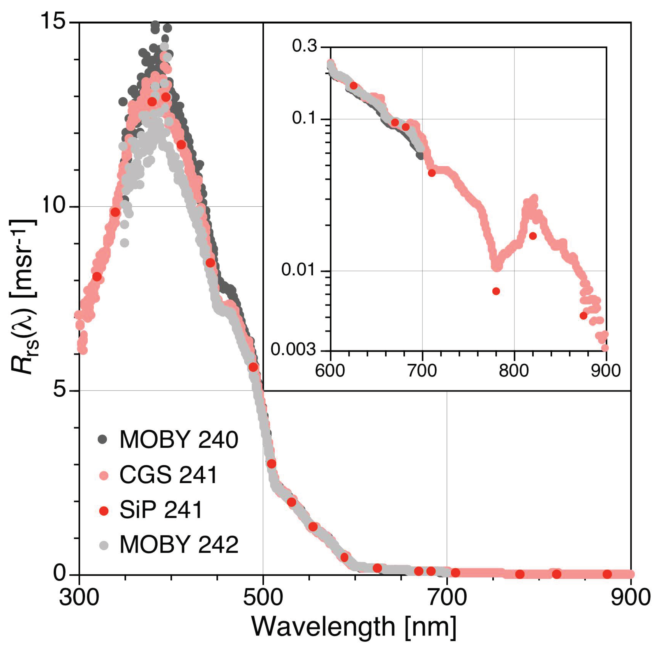
  • A verification comparison of hyperspectral C-PHIRE and MOBY data products; and
  • A verification comparison of the hyperspectral MOBY and multispectral microradiometers.
The validation and verification steps include multiple comparisons. The hyperspectral data were converted to the microradiometer wavebands and the microradiometer data products were derived from the companion C-PHIRE microradiometers or a separate C-OPS instrument. The data products compared include the following or a restricted subset as determined by the source (with wavelength omitted for brevity): E s , E d , and L u calibration and lower-level data products (Section 3.1 and Section 3.2, respectively), plus higher-level data products as applicable, e.g., R rs (Section 3.3) along with band ratios used for the algorithms (Section 3.4) considered herein.
Ref. [19] demonstrated the use of microradiometers to provide high quality AOP data. Improvements to the in-water approach were documented by [9,15,16,17] with the resulting improvements to higher-order applications, e.g., algorithms, demonstrated by [10,27]. Similar accomplishments in above-water applications of microradiometers were presented by [30,32,33,34].
The calculations between two data sources, X and Y, are based on an unbiased perspective, i.e., both sources are considered equally correct. The hyperspectral data can involve thousands of pixels, so the spectral components are simplified into the five aforementioned spectral domains, hereafter λ D , to make the results briefer to present without any loss in significance. The boundaries for the domains are as follows: UV 300–399 nm, Blue 400–499 nm, Green 500–599 nm, Red 600–699 nm, and NIR 700–900 nm, wherein the middle three represent the larger VIS domain. In keeping with the spectral width of the other domains, the NIR is also considered as NIR1 (701–799) and NIR2 (800–900). The total number of observations within a particular spectral domain is denoted N D .
Two statistics are used to determine the efficacy of the data obtained with C-PHIRE radiometers and thereby validate their applicability to CVR radiometry. The first statistic is the relative percent difference (RPD), ψ , which uses a signed difference to reveal a potential bias in performance:
ψ ( λ D ) = 200 N D i = 1 N D X i Y i X i + Y i ,
where the index i is restricted by λ D . RPD values can cancel when summed and are, therefore, inappropriate for accuracy estimates. Consequently, accuracy (or uncertainty) is estimated using the absolute percent difference (APD), ϕ :
ϕ ( λ D ) = 200 N D i = 1 N D | X i Y i | X i + Y i ,
which is also used to estimate overall spectral uncertainties spanning UV–NIR.
To facilitate the presentation of results, a compact notation is used wherein the variable of interest is combined with superscripts and a shorthand notation for the instrument detector to document the data product and source. For the former, E s , E d , and L u are the basic variables. A C superscript indicates calibration data, and the 0 and 0 + superscripts denote derived products from field data, as appropriate. Consequently, E s C , E d C , and L u C are calibration data and the corresponding data products from field data are E s 0 + , E d 0 , and L u 0 .
To compare a hyperspectral and multispectral data sources, the former is converted to the latter using one of two band conversions: (a) the spectral response function (SRF) of the multispectral individual bandpasses are applied to convert the hyperspectral data to equivalent multispectral wavebands; and (b) the bandwidth of the multispectral channels are used to average the hyperspectral data to equivalent multispectral wavebands. The two conversions are considered herein because of the focus on COTS instruments for which SRF characterizations are not always provided with an instrument suite.
To uniquely identify the instrumentation involved in a comparison of data products, the following codes are established:
PHY
  The C-PHIRE hyperspectral data;
PAH
  The C-PHIRE hyperspectral data converted to averaged wavebands;
PBH
  The C-PHIRE hyperspectral data converted to bandpass wavebands;
PMS
  The C-PHIRE multispectral data;
OMS
 The C-OPS multispectral detector data;
MHY
 The MOBY hyperspectral data; and
MBH
 The MOBY hyperspectral data converted to bandpass wavebands.
To complete the shorthand notation, the applicable instrumentation being compared and their codes are placed to the right of the variable and data source with the two sides separated by a vertical bar. The instrumentation codes are placed one over the other with the numerator representing X and the denominator Y in (2) and (3), i.e., the reference instrument in the difference is the denominator.
A comparison of the E d ( 0 , λ ) data products derived from contemporaneous C-PHIRE and C-OPS profiles for the multispectral detector data, for example, would be denoted E d 0 | OMS PMS . Similarly, a comparison of the same data product for the C-PHIRE hyperspectral data and the C-OPS multispectral data would be E d 0 | OMS PBH , wherein the C-PHIRE hyperspectral data are converted to a bandpass product using the applicable SRF for the C-OPS channels to produce the equivalent 10 nm data as C-OPS.

3. Results

The focus of this study is to evaluate the efficacy of hybridspectral radiometers to derive AOP data products. The approach uses a combination of calibration and in situ data wherein the different detector systems are compared as a function of increasing data product complexity. Data product complexity in this context is with respect to the baseline performance on an optical bench as well as the increasing number of terms used to derive a data product with the source terms of N1 in (1) being the simplest, e.g., E s , E d ( 0 ) , and L u ( 0 ) . Data product complexity increases as N1 is more completely expressed, e.g., starting with the use of L W and R rs , and then including the N2 and N3 terms in (1).

3.1. Validation Using Calibration Data Products

The calibration bench is considered the simplest and most controlled use of the instrumentation. The principal reason for this is the observed flux is essentially unvarying, because the light source is established by powering a lamp using computer feedback through precision components, and the instrumentation is positioned in a laboratory using a fixed and reproducible geometry within a properly baffled environment to minimize stray light. In addition, all targets and sources are traceable to the National Institute of Standards and Technology (NIST) in strict compliance with the Protocols. Ref. [16] provides extensive documentation regarding C-PHIRE characterization and calibration, so only a brief summary based on the most important elements is presented here.
The parameters of interest are the calibrated spectral responses for the solar reference ( E s ), plus the in-water downward irradiance ( E d ) and upwelled radiance ( L u ) radiometers as a function of the spectral domains established in Section 2.6, i.e., E s C ( λ D ) , E d C ( λ D ) , and L u C ( λ D ) , respectively. The statistical comparisons considered are between the hyperspectral and multispectral detectors in each radiometer, wherein the former yields two data products to be compared to the latter, as follows: PAH is the band-averaged hyperspectral data without use of the multispectral SRF data, and PBH is the bandpass hyperspectral data with the multispectral SRF data applied. Because the comparisons are based on observations obtained on the optical bench, the only correction applied is to remove the dark current offset, e.g., no immersion factors are applied. The removal of the dark currents is different for the hyperspectral and multispectral detector systems.
For hyperspectral CGS measurements, the shortest wavelengths wherein no detectable natural radiation exists—denoted 245 < λ s < 290 nm—are used to determine the dark current offset and then to correct the light measurements for wavelengths above 290nm on a measurement-by-measurement basis. This correction is possible because tests indicate that changes in the dark offset are nearly independent of the spectrograph pixel. Furthermore, this procedure is reliably stable and does not require the aperture to be capped, so it can be done under all illumination conditions. The multispectral microradiometers require a separate procedure to determine the dark current offset, as follows: (a) an opaque cap is placed on the aperture; (b) the instrument suite is sequentially configured through commands issued to the instruments to set each of the three gain stages for all microradiometers, and dark data are collected for a specified number of observations (usually 1024 in the field, but less in the laboratory where environmental variables are minimized) at each gain stage; and (c) the dark current offsets are subsequently subtracted from all subsequent light observations. Although this process is used during data acquisition and data processing, the latter uses more sophisticated tools, e.g., power spectral density analysis, to detect and apply corrections for trends and anomalies.
An optimal measurement scenario for validating the two detector systems in a C-PHIRE radiometer can be conducted in the laboratory on an optical bench wherein sources of variance are minimized. To compare the hyperspectral and the microradiometer data, the former are converted to the equivalent 10 nm wavebands for the latter. Two hyperspectral-to-waveband conversion schemes are presented in Table 1 for data obtained during a calibration of the three C-PHIRE radiometers. The Table 1 results indicate the agreement between hyperspectral and multispectral instrument systems is quite close when using both types of band conversions considered. As expected, the bandpass conversion invoking the application of the SRF improves convergence in all spectral domains albeit with a magnitude that is similar to or lower than the uncertainties inherent to radiometric calibration activities (e.g., NIST lamp scales of spectral irradiance).
One significant reason for the close convergence within and between instruments in Table 1 is the smooth spectral output of a calibration lamp. With high-quality instrumentation (i.e., large dynamic range, high sensitivity, low-noise electronics, and properly designed blocking to minimize stray light and out-of-band contributions), this convergence would be expected to translate to above- and in-water field measurements, in particular, when there are limited spectral features within the passbands of the multispectral system. In environments where there may be significant spectral features within the multispectral wavebands the application of the SRF in calibration and data processing would be expected to improve the accuracy and convergence of the two systems. The recommended wavebands in the Protocols for ocean color research are spectrally positioned to avoid parts of the spectral domain with high variability (from principally a case-1 perspective). Regardless of whether or not an SRF is applied during calibration and data processing, it is a vital part of the instrument characterization to verify the blocking efficacy for out-of-band and stray light issues.
The overall agreement for the two detector systems in the three instruments within Table 1 as a function of the averaged and bandpass conversion schemes is ϕ ¯ = 1.0 % and ϕ ¯ = 0.9 %, respectively, i.e., the bandpass approach yields lower uncertainties. The resulting 1% threshold is considered the best achievable agreement between two detector systems exposed to the same flux under stable conditions in the field, as well as the best possible agreement in derived data products, i.e., what is notionally referred to as 1% radiometry [19]. This notional concept is in addition to the CVR thresholds presented in Figure 1. The Table 1 results indicate the blocking within C-PHIRE instruments is sufficient to minimize stray light and out-of-band issues and thereby ensure 1% radiometry, because uncomplicated procedures yield agreeable results. Because of the close agreement between the averaged and bandpass results in Table 1, only the bandpass approach is used hereafter, because it is more robust in the presence of spectral features in the more complex water masses considered.

3.2. Validation Using Lower-Level Data Products

Thrusters stabilize the backplane in two axes to improve the planar geometry of optical apertures, which increases data retention and allows the pressure transducer port to be driven above the sea surface for profile-by-profile pressure tares. For this study, the tilt of the in-water apertures within the extrapolation interval was within ±2.5 , with an average value of 0.9 . Hydrobaric buoyancy plus application of adaptive thruster control slows backplane vertical motion near the sea surface thereby improving the vertical sampling resolution (VSR), which is defined as the extent of the extrapolation interval divided by the number of data points retained within [27]. For this study, the VSR for the E d and L u instruments differ because the latter has the reverse orientation of the former. In addition, the TOW-FISH is subjected to more forces than a C-OPS, so these two instrument suites had different VSR values. A spectrometer generally samples slower than a microradiometer which further distinguishes the VSR between instruments. For this study, a VSR of less than 1.5 cm was required for all in-water comparisons. The average VSR for microradiometer data products was 0.7 cm, although a few profiles associated with testing dedicated thruster control had VSR values less than 1 mm. The contemporaneous average VSR for hyperspectral data products was 1.1 cm.
More than 100 up and down C-PHIRE profiles were obtained for this study, but a little more than half of them involved trials to confirm performance parameters to document an operational technology readiness level (TRL) value of nine [16], which is the maximum. The performance trials frequently made one or more of the optical data noncompliant with VSR requirements, e.g., adaptive thruster tuning, power consumption verification, simulated emergency response, etc. The total number of comparisons is 61 for E s ( λ ) comparisons, 42 for C-OPS, and 48 for C-PHIRE. The datasets are not equal, because some trials excluding compliant profile data still allow solar irradiance comparisons and because the C-PHIRE casts are more numerous than the contemporaneous C-OPS validation casts. The onset or aftermath of severe weather events shortened the length of all deployments. The longest deployment was eight days off the coast of Puerto Rico, but the influence of severe weather nonetheless provided significant and always successful testing of all components and subsystems.
The variables of interest in regard to lower-level data products are E s 0 + ( λ D ) , E d 0 ( λ D ) , and L u 0 ( λ D ) , which are ordered as a function of increasing processing complexity, respectively, are as follows: (a) the E s 0 + ( λ D ) data have the fewest corrections and the highest flux, because the SV3 10 d mission is to collect data during clear skies and fair weather; (b) the E d 0 ( λ D ) data are similarly stable to E s 0 + ( λ D ) except for the presence of in-water attenuation, wave focusing, and planar tilting; and (c) the L u 0 ( λ D ) data are similarly stable to E d 0 ( λ D ) except for the significantly dimmer signal and the need for a self-shading correction.
A comparison of the selected variables derived from the multispectral and hyperspectral detector systems is presented in Table 2. Two sets of results are considered, wherein the multispectral data are derived from C-PHIRE and contemporaneous C-OPS observations (left three columns) and the hyperspectral CGS data are converted to PBH bandpass data (right three columns). For both types of comparisons, the best overall agreement, i.e., lowest ψ ( λ D ) and ϕ ( λ D ) values, follows a E s 0 + ( λ D ) , E d 0 ( λ D ) , and L u 0 ( λ D ) lowest-to-highest progression. The minimum overall ψ ( λ D ) and ϕ ( λ D ) values are for the multispectral comparisons with the hyperspectral comparisons typically maximal and sometimes significantly higher. For the three variables and both types of comparisons, the irradiance variables always satisfy the notional 5% calibration threshold (Figure 1) and the solar irradiance comparisons are frequently within or close to the notional 1% radiometry threshold established in Section 3.1 (removal of the NIR bands results in overall statistics much closer to 1%). For the UV and VIS wavelengths, the radiance differences are similarly compliant with the notional 5% calibration threshold, but not always for the NIR. Omitting the NIR2 wavebands (820 and 875 nm) yields an overall L u 0 ( λ D ) that is within 5.0%.
Omitting the NIR2 wavebands is justified because the Protocols do not specify an uncertainty requirement for NIR2 wavelengths. In addition, as presented below, the MOBY data obtained from SeaBASS extend from approximately 350–700 nm and the majority of the other hyperspectral in-water data available in SeaBASS span approximately 400–800 nm. Smaller collections of more expansive data are available, and these data extend from about 350–800 nm. In all cases, however, the NIR2 domain is not present. Based on the absence of NIR2 wavelengths in SeaBASS submissions and performance requirements within the Protocols, it appears reasonable to qualify the NIR2 results as is performed herein. The Protocols also do not specify an uncertainty requirement for UV wavelengths, but the recurring in-water SeaBASS submissions containing UV wavelengths, even if the data do not span the entire UV-A domain nor contain UV-B wavelengths, suggest UV wavelengths are important to CVR activities, as documented for next-generation missions [3].
Another progression that is evidenced in Table 2 is the order of the ϕ values as a function of the spectral domains. In the Table 2 comparisons and using ϕ as a proxy for uncertainty, the smallest uncertainties are found in the Blue and Green domains with larger uncertainties in the UV and Red domains, culminating with the largest uncertainties in the NIR. In regard to the notional CVR uncertainties presented in Figure 1, the 5% calibration threshold is satisfied for all domains except the NIR involving a hyperspectral PBH data source, although the NIR multispectral PMS and OMS comparisons are compliant or nearly so. The NIR2 domain is the principal source of degradation in overall average uncertainty values, and if NIR2 results are omitted, overall average uncertainties are less than the notional threshold of 15% for validation using a hyperspectral data source. The NIR domain provides the only evidence of a potentially significant and systematic bias, but only for comparisons involving a hyperspectral sensor.

3.3. Validation and Verification Using Higher-Level Data Products

The higher-level data products considered herein are K d ( λ ) and R rs ( λ ) , which are so designated because both parameters are direct inputs for common algorithms, aspects of which are considered in Section 3.4. The R rs ( λ ) presentation includes a comparison with MOBY. Because of severe weather, the MOBY data do not meet the temporal and spatial requirements for contemporaneous matchups and are considered as a source of verification (Section 2.6) rather than validation, but they are considered with the same comparison statistics. As noted in Section 2.2, E d ( 0 , λ ) and, thus, K d ( λ ) , are part of the process for determining the extrapolation interval to derive L u ( 0 , λ ) , which is subsequently used to derive L W ( λ ) . Both K d ( λ ) and L W ( λ ) are directly connected to lower-level data products in Table 2, as follows: (a) K d ( λ ) is based on the slope of E d ( λ ) in the extrapolation interval used to determine E d ( 0 , λ ) ; and (b) L W ( λ ) is simply a constant (0.54) times L u ( 0 , λ ) . This means the ψ and ϕ statistics for L W ( λ ) are not presented again.
The coherence between data products that only differ by constant terms is also applicable to the concept of comparing R rs ( λ ) and L W ( λ ) N data products from two C-PHIRE detector systems. Consequently, L W ( λ ) N data products from the two C-PHIRE detector systems are not compared here, because these results will be essentially the same, i.e., the N2 and N3 terms in (1) for the two C-PHIRE detector systems will be the same, thereby leaving only the R rs ( λ ) parameter as the source for differences in the comparisons. Comparisons involving L W ( λ ) N are deferred to Section 3.4, wherein comparisons involving data sources and implementing different algorithms using R rs ( λ ) and L W ( λ ) N data products are presented.
Statistical comparisons involving K d ( λ ) and R rs ( λ ) from C-PHIRE and MOBY sensors are shown in Table 3 with both multispectral and hyperspectral data sources considered. The Table 3 data confirm the following results seen in Table 2:
  • Data products based on the higher flux measured by an upward-pointed irradiance instrument ( K d ) have smaller differences than those based principally on the lower flux of a downward-pointed radiance instrument ( R rs );
  • The K d differences are only a little larger than the best possible differences determined on the optical bench (Table 1);
  • Comparisons between multispectral data sources (e.g., PMS and OMS) have smaller differences than those involving hyperspectral data (e.g., PBH and MBH);
  • The smallest differences are found for the VIS domain; the neighboring UV and NIR domains have larger differences, with the NIR having the largest;
  • There is little evidence of a significant and systematic bias as a function of spectral domain or sensor type except for NIR comparisons involving a hyperspectral sensor.
For the last result, the hyperspectral sensors are distinguished by fewer decades of dynamic range and a slower sampling rate when pointed at a dark target than the multispectral sensors, so potential biases in hyperspectral data products are anticipated when the signal-to-noise ratio (SNR) is small, e.g., in the NIR domain when observed with an L u radiometer.
The superior results obtained for the K d ( λ ) comparisons suggest algorithms using K d ( λ ) as an input variable are likely more accurate and more versatile. This improved accuracy was documented by [19,27,33]. The enhanced versatility is the result of the derivation procedures not requiring a calibrated instrument—all that is required is the instrument remain suitably stable over the time period of the experimental activity, which at a minimum would be the time to obtain an E d ( z , λ ) profile. For the optical results presented herein, the C-PHIRE data products were derived in the upper 1–2 m of the water column with a vertical extent of the average extrapolation interval extending to 1.6 m. In comparison, the average vertical extent of the extrapolation interval for the multispectral C-OPS data extended to 0.9 m. The relatively shallow extrapolation intervals ensure a rapid acquisition schedule. The stability of an instrument over the short time period spanning a typical field campaign lasting several weeks does not present a significant challenge for optical field instruments built with microradiometers, which use ion deposition filters [35].
In regard to hyperspectral and multispectral comparisons, Figure 3 shows MOBY data from two days (SDY 240 and 242 in 2016) bracketing a day of severe weather (SDY 241) wherein C-PHIRE hyperspectral (CGS) and multispectral (SiP) profiles were obtained when the SV3 was deployed close to the MOBY site in a protected lee of the island of Lana’i (Hawaii). For the common spectral regions, the largest signal variability is in the UV domain followed by the Red domain. In addition, the C-PHIRE data show there is also variability in the NIR for the hyperspectral data and the comparisons with respect to the multispectral data. These are the three domains showing the largest comparison differences in Table 2 and Table 3.
The hyperspectral CGS and multispectral SiP data shown in Figure 3 are for one profile out of five. The other four profiles were not displayed in Figure 3 to improve the clarity of the figure, but all the data are represented in the prior tables involving PBH and PHY results (Table 2 and Table 3), as well as any subsequent presentation below.

3.4. Algorithm Output Validation

Two common ocean color parameters that are derived from optical observations using different input parameters are a CDOM ( 440 ) and C a . The former is estimated using the end-member analysis (EMA) approach [19] based on algorithms derived in [27,33] using K d ( λ ) and L W ( λ ) N data products, respectively. The latter is estimated using the Ocean Color Four (OC4) SeaWiFS algorithm. The most recent formulation for OC4 was obtained from NASA (https://oceancolor.gsfc.nasa.gov/atbd/chlor_a/, 28 December 2021). In both algorithms, band ratios of optical parameters are used as inputs, but the a CDOM ( 440 ) algorithm can use both K d ( λ ) and L W ( λ ) N , whereas OC4 uses R rs ( λ ) . The single-band versions of the EMA a CDOM ( 440 ) algorithm [30] are not considered. The combination of band ratios for the selected algorithms provides an analysis with a diverse set of input variables and spectral attributes.
Table 4 presents the comparison statistics for the output of the algorithms based on the input variables determined from two data sources, as identified previously for Table 2 and Table 3. The input variables are band ratios of K d ( λ ) , R rs ( λ ) , or L W ( λ ) N derived from contemporaneous observations obtained from two different instruments with the same sensor technology (PMS and OMS) or simultaneous observations obtained from two different sensors in the same instrument (PBH and PMS). The Table 4 analysis does not validate the algorithms—it validates whether the inputs from different data sources produce output variables in keeping with the notional uncertainties in Figure 1, i.e., the most expansive result is in agreement for calibration, which is within 5%.
All the absolute ( ϕ ) differences in Table 4 are within 5%, with the smallest differences associated with the K d ( λ ) input variables. In addition to being the variable with the best agreement in Table 3, K d ( λ ) was also shown by [30] to provide superior wavelength-by-wavelength a CDOM ( 440 ) estimation than L W ( λ ) N for single-channel sensors. The largest differences in Table 4 are associated with the hyperspectral bandpass PBH and multispectral PMS data for the R rs ( λ ) and L W ( λ ) N input variables. In all cases, there is no significant evidence of bias, and the largest differences involve the derivation of input variables from hyperspectral data.

4. Discussion

Incrementally persistent advances in remote sensing capabilities and algorithm designs are anticipated to extend the applicability of ocean color observations from oceanic to coastal and inland waters. This trajectory in ocean to aquatic remote sensing capabilities is demonstrated by the goals of the PACE mission, which is expected to provide hyperspectral imagery with an expanded spectral range and to improve algorithmic capabilities for optically complex ecosystems. Successfully leveraging the potential application for PACE observations will require accurate and cost-effective (i.e., autonomous) radiometry that matches PACE spectral configuration for in situ activities spanning all tiers of the CVR triad. At present, in situ capabilities that meet this requirement are lacking. For example, the SeaBASS repository does not contain datasets spanning the spectral range used in this study, even though this study was designed in anticipation of PACE radiometric capabilities.
The transition from oceanic to coastal and inland water bodies also corresponds to an increased heterogeneity of potential water body targets (Figure 1). As such, an increased breadth of in situ measurements is required, which will likewise require either increased funding for manual sampling activities or a community effort to advance automated sampling capabilities. Presently, activities to support autonomous ocean observing capabilities are increasingly common, demonstrated for example by expanded radiometric capabilities for Argo floats [14], algorithmic improvements to reduce costs in drone and float platforms [30], and autonomous airborne systems for opportunistic monitoring of inland bays and lakes [10,30,32,33].

4.1. Autonomous Observations of Aquatic Ecosystems Using an SV3 Platform

The operational demonstration (TRL 9) of the SV3 remote sensing platform in this study provided increased mobility compared to larger (usually stationary) systems, and also conferred advantages for validation activities compared to smaller platforms such as a float or drone, as follows and documented in more detail by [16]: (a) propulsion by wave energy allowed spatially targeted sampling—as opposed to a float in which sampling locations are dictated by currents or winds—without depleting battery reserves for the scientific payload and while continuously moving air and water over the respective apertures to minimize biofouling; (b) steering by the thrudder enabled directional control to adhere to solar geometry requirements and enhanced propulsion was never required, although it provides significant risk management opportunities; (c) the float provided sufficient buoyancy and stability to support a sophisticated payload, including a data acquisition computer, solar panels, plus an instrument package with a surface reference irradiance instrument suite with a shadow band, PAR sensor, GPS, and WiFi antennas (Figure 3); and (d) power supplied by the float plus an additional payload battery system for the profiler allowed all sampling and vertical profiling to complete successfully while remaining in compliance with the power budget.
Despite the increased size of the SV3 and profiler payload compared to that of an autonomous float or drone, the SV3 was successfully deployed for long periods due to the solar power array combined with added battery storage housed in the Float. The system was transported by truck almost fully assembled (California) and by aircraft completely disassembled (Hawaii and Puerto Rico) without mishap. SV3 mobilization requires modest shore facilities. For the Lana’i deployment, the SV3 was assembled outside in a picnic area next to a parking lot and then rolled down a driveway onto a dock for subsequent loading onto a small boat. This flexibility also enabled the rapid relocation of the system before the onset of severe weather (Hawaii) and to sample the early stages of a HAB research opportunity (Monterey Bay). Impact risks from ships were reduced by the AIS system combined with the thrudder capabilities, although examples of other SV3 systems that have survived a ship collision with minimal damage were reported. Risks of vandalism were reduced compared to a stationary platform, because the system’s variable location and minimal above-water profile reduced visibility of, and attention to, the SV3 system (there was no evidence of a random encounter with a commercial or recreational boater).
Uncertainties due to variability in sky state were mitigated by the addition of a shadow band (which allows the derivation of atmospheric data products), combined with the surface irradiance measurements (including PAR) mounted on the float cover plate. During the 8 d deployment off the Puerto Rico coast, the float was successfully cleaned by a field team that visited the SV3 system by small boat. For missions lasting longer than 10 d, biofouling of the profiler will likely be an issue requiring mitigation. Although many solutions are possible, microradiometers provide a unique built-in opportunity. It is possible to replace a SiP microradiometer with a circuit having the same form factor and a compliant architecture designed to control a UV light-emitting diode (LED). When the LED is powered, the LED emits UV light intended to hinder or eliminate the growth of organisms on the radiometer aperture
In regard to comparing this study to the literature, a similar technological solution can be artificially constructed by considering the instrumentation of autonomous floats equipped with either multispectral [36] or hyperspectral [37] radiometers. Ref. [36] reported a precision of approximately 5% for L W at 412, 443, 488, and 555 nm, i.e., the Blue and part of the Green domains. The comparable wavelength ranges in this study are equal to or better than this value (Table 2), thereby confirming an ability to generate high fidelity measurements from an autonomous vehicle that satisfy the notional calibration threshold. There are pros and cons to Eulerian versus Lagrangian sampling, but the ability to conduct command and control of the vehicle and profilers in real-time is a significant advantage compared to that of purely autonomous floats. Extending the comparison to the hyperspectral domain, Ref. [36] estimated optimal errors of 3.1–5.8% for the wavelength range 380–665 nm, with an achieved accuracy of approximately 10% for a prototype hyperspectral float. Across all spectral domains, the uncertainty reported here was 3.5% (for a considerably wider spectral range), demonstrating that this technology can provide data products with the highest possible fidelity from field measurements. The uncertainties presented herein are also well within recently reported comparisons of MOBY and VIIRS matchups [38], demonstrating that the SV3 platform can provide comparable calibration and validation data for satellite matchups but with a potential global footprint.

4.2. Validation and Verification Comparisons

Observations obtained using C-PHIRE instruments leveraged similar advanced instrumentation, i.e., microradiometer technology, as C-OPS, documented in earlier publications, e.g., Refs. [10,15,16,17,19,27,30,39]. Comparison between the multispectral and hyperspectral calibration data products (Table 1) indicate overall agreement across all spectral domains to within approximately 1%. Besides the low uncertainties derived for the hyperspectral data products, additional benefits were conferred from simultaneous hybridspectral (multispectral and hyperspectral) observations, and these benefits are discussed in more detail below (Section 4.3).
Comparisons between simultaneous C-OPS and C-PHIRE field observations (Table 2) indicate uncertainties in the multispectral data products agree on average to within 2.0%, when excluding the NIR2, which is a slight but anticipated increased from the differences shown in Table 1. Hyperspectral observations are slightly worse, although results for the VIS domain and the irradiance instruments are similar. The downward-pointing radiance instruments indicate the greatest differences, particularly in the UV and NIR domains, where signal levels can be significantly lower, e.g., in the open ocean for the NIR and in high turbidity waters for the UV.
For higher-level data products (Table 3), comparisons of field observations are improved, particularly for data products that are primarily derived from E d , rather than L u , observations. Verification with MOBY indicates uncertainties to within 5%, except for within the UV and NIR domains, although MOBY comparisons were restricted to a narrower spectral range of 380–710 nm (with the latter extrapolated from 695–699 nm). Derived products including a CDOM ( 440 ) and C a (Table 4) provide uncertainties less than 5%. For comparison, Ref. [34] indicated an uncertainty less than 17.5% for C a was acceptable, and noted a typical global uncertainty is 5%. For a CDOM ( 440 ) Ref. [27] reported uncertainties of 1.2–6.2% for a global dataset derived using EMA. In both cases, the data presented here are within these uncertainty ranges.
Averaging by spectral domain, all validation and verification measurements presented herein were within the notional 5% calibration uncertainty threshold adopted in Figure 1, with the exception of the NIR domain, with average uncertainties ( ϕ ¯ ) as follows: UV 2.9%; Blue 2.0%; Green 1.3%; Red 2.8%; and NIR 8.3%. If the MOBY verification comparisons are removed, uncertainties within the UV and NIR domains (i.e., the spectral end members) are reduced to 2.2% and 7.6%, respectively. Across all spectral domains, the average uncertainty is 3.5%. If the incomplete UV and extrapolated NIR results for MOBY 710 nm data products are removed, the average uncertainty is reduced to 3.2%. Furthermore, if the more challenging NIR2 domain is omitted from the overall NIR averages, the average uncertainty for NIR1 is ϕ ¯ = 2.9 % , i.e., the NIR1 results are almost the same as the Red domain results ( ϕ ¯ = 2.8 %).
These results show that the lowest uncertainties are in the VIS wavelengths where the illumination flux is maximum. The neighboring UV and NIR domains have higher differences, with the NIR having the highest. The greatest challenge is for NIR2, particularly for the hyperspectral data which relies on a detector system with fewer decades of dynamic range and typically a slower sampling rate (which results in a degraded SNR and degraded VSR, respectively). Opportunities to mitigate low signal difficulties for hyperspectral measurements based on concurrent multispectral measurements are discussed in Section 4.3.
The variety of environments successfully sampled using the SV3 and C-PHIRE instrumentation demonstrate the benefits of using a moveable platform for validation and research activities. Relative differences in uncertainties between the NIR, VIS, and UV domains are also a function of the optical complexity of the targeted water mass. For example, the majority of data obtained for the comparisons presented herein were in water masses representative of the transition between oligotrophic and mesotrophic waters, i.e., 0.10   <   C a   <   0.12 mgm 3 . If only the oligotrophic portions of the data are considered—consistent with the calibration perspective favoring water mass homogeneity— the comparisons produce lower uncertainties in the UV domain, but with simultaneous degradation of the NIR data products. The opposite—increased uncertainties in the UV and decreased uncertainties in the NIR—are found if only the eutrophic portion of the dataset are considered. These large-scale differences are expressed in all comparisons, because the instruments involved are either in near proximity to one another or in the same housing, so environmental influences are significantly the same for all sensors at the time of measurement wherein one-on-one comparisons are computed.

4.3. Advantages of the Hybridspectral Perspective

Hyperspectral data products obtained with the SV3 package were observed simultaneously with multispectral data products, a combined architecture defined as hybridspectral. This hybridspectral architecture confers multiple advantages, including useful redundancies in radiometric measurements. For example, each detector system can be used to continuously monitor the other to detect anomalous performance and drift. Additionally, the dynamic range of multispectral microradiometers can provide valid cast data in light-limited or highly attenuated water masses wherein a spectrograph may not be adequate, particularly for the spectral end members. Although system failures with microradiometer instruments were found to be exceedingly uncommon, all technologies are susceptible to failure due to routine or irregular mishaps, including stressors induced by user errors. In the case of a failure of a multispectral waveband within a hybridspectral system, hyperspectral data products provide interpolation information to restore degraded or missing measurements between two adjacent, surviving microradiometer channels. In the case of a failure of the spectrograph, the multispectral instrument will continue to provide data at the primary CVR wavebands of interest for the scientific community.
Another potential application of the hybridspectral capability is to leverage the sampling rate capabilities of the multispectral instruments to improve, e.g., tune, the hyperspectral data products. This scenario can be demonstrated by considering Figure 3, in which hyperspectral and multispectral observations are overlaid, along with more spectrally limited MOBY observations for completeness. In this example, the hyperspectral observations are artificially brightened compared to the multispectral observations within the NIR domain. The hyperspectral instruments, which have increased noise contamination relative to signal level, i.e., are more signal limited than the multispectral instruments, are anticipated to routinely provide steeper attenuation slopes for L u and, therefore, produce brighter estimates of L u ( 0 ) due to noise contributions to the L u profile.
Correction of the slower hyperspectral observations using the more rapid multispectral observations with high SNR can prevent potential biases, including the difficulty of using spectrometers to make measurements in extreme waters. For example, in optically complex case-2 waters the microradiometers require a lesser vertical sampling extent to accurately derive K, which can then be used to extrapolate the fewer hyperspectral data (wherein a greater vertical sampling extent is needed to obtain comparable data products). The concept of mitigating hyperspectral sampling deficiencies with microradiometers was not evaluated in this study, because of the absence of independent data with applicable spectral properties to create a comparison dataset. The optical package and integration scheme was designed with an agnostic platform perspective, so the approach described in this study is intended to be applicable to any capable USV platform for future studies.

5. Conclusions

Recalling the calibration, validation, and research (CVR) triad, calibration activities historically focused on oligotrophic waters with restricted sampling requirements (Section 1, e.g., items C1–C3), whereas validation and research activities expanded to include waters with increased optical complexity, including coastal and inland water bodies. The verification observations presented herein (i.e., with the marine optical buoy (MOBY) platform) considered oligotrophic waters, while validation comparisons presented spanned oligotrophic, mesotrophic, and eutrophic waters. Research sampling included harmful algal bloom (HAB) conditions in Monterey Bay plus a eutrophic inland lake. The range in environments sampled was enabled by the portability and robustness of the SV3 plus optical package combination. The commercial-off-the-shelf (COTS) hybridspectral system described herein satisfied the notional 5% threshold for calibration quality (Table 1, Table 2, Table 3 and Table 4) across a global dynamic range, and it was shown to meet the most challenging CVR requirements for next-generation missions in all water masses of interest. The ability to deploy the optical instruments on a COTS self-contained unmanned surface vessel (USV) that retains command and control capabilities provides more versatility than other autonomous platforms. The comparison with the MOBY data demonstrates that the COTS technology used in this study provides comparable data, but with a global applicability, i.e., it is not restricted to an oligotrophic water mass.
Next-generation sensor configurations are anticipated to enable remote observations of global—rather than oceanic—water bodies. This transition in remote sensing from primarily homogeneous oligotrophic to routinely heterogeneous coastal and inland waters (Figure 1) requires advanced in situ instrumentation to support concurrent advances in algorithm design to overcome the historical case-1 versus case-2 perspective [10,39]. In regard to the ensuing continuum of optical complexity, three considerations appear important. First, global aquatic observations needed to support this transition must be automated to increase the breadth of coverage, demonstrated herein by leveraging the capabilities of the SV3 platform. Second, increasing the availability of validation-quality in situ observations will benefit from the adoption of multiple technological improvements to in-water measurements. Third, this study demonstrated that multispectral, hyperspectral, and hybridspectral instruments all provide data useful to CVR activities, but the hybridspectral approach improves data sets by providing a broader and compliant spectral range and anchoring the less sensitive spectrometer to the more sensitive microradiometers.
For the in situ datasets presented herein, hybridspectral sampling (Section 4.3) provided redundancy in the case of a potential microradiometer failure and could be used in the future to reduce bias in hyperspectral measurements, particularly in the signal-limited water bodies involving the UV and NIR spectral domains. Vertical sampling resolution (VSR) was improved by thruster-assisted profiling, increased sampling rates, and hydrobaric buoyancy to optimize profiler descent and ascent rates. Technologies that improve VSR help to mitigate basic challenges of in-water radiometry, including depth limitations, shallow attenuation scales, and wave-focusing effects. These advances had been documented previously for handheld or stationary profilers, but were not yet evaluated for an automated in-water activity relevant to satisfying requirements for next-generation CVR exercises in oceanic and aquatic remote sensing.

Author Contributions

Conceptualization, S.B.H. and H.F.H.; methodology, S.B.H., R.N.L. and R.M.K.; software, S.B.H. and H.F.H.; validation, S.B.H., H.F.H., R.N.L., R.M.K. and K.S.; formal analysis, S.B.H., H.F.H. and R.N.L.; investigation, S.B.H., H.F.H., R.N.L., R.M.K. and K.S.; resources, S.B.H., R.M.K. and K.S.; data curation, S.B.H., R.N.L., R.M.K. and K.S.; writing—original draft preparation, S.B.H., H.F.H., R.N.L. and R.M.K.; writing—review and editing, S.B.H., H.F.H., R.N.L., R.M.K. and K.S.; visualization, S.B.H., H.F.H. and R.N.L.; supervision, S.B.H.; project administration, S.B.H.; funding acquisition, S.B.H., R.M.K. and K.S. All authors have read and agreed to the published version of the manuscript.

Funding

This work was supported by the National Aeronautics and Space Administration (NASA) as part of planning for the Aerosol, Cloud, Ecosystems (ACE) plus PACE satellite remote sensing missions (NNX14AT67G and NNX14AT40G), as well as the Japan Aerospace Exploration Agency (JAXA) Second-Generation Global Imager (SGLI) launched aboard the Global Climate Observation Mission-Climate (GCOM-C) Shikisai satellite (JX-PSPC-530171).

Data Availability Statement

The data supporting the conclusions of this article will be made available by the lead author, without undue reservation.

Acknowledgments

The high level of success achieved in the field work used for this study established a foundation of understanding that was the direct consequence of commitments from individuals who contributed unselfishly to the work involved (e.g., calibration, acquisition, sampling, processing, and analysis). The scientists included (alphabetically) R. Armstrong, J. Brown, C. del Castillo, T. Comer, J. Morrow, and K. Negrey; their dedicated contributions are gratefully acknowledged.

Conflicts of Interest

The authors declare no conflict of interest. The funders had no role in the design of the study; in the collection, analyses, or interpretation of data; in the writing of the manuscript, or in the decision to publish the results.

References

  1. Hooker, S.B.; Esaias, W.E. An overview of the SeaWiFS project. Eos Trans. Am. Geophys. Union 1993, 74, 241–246. [Google Scholar] [CrossRef]
  2. Asrar, G.; Greenstone, R. 1995 MTPE/EOS Reference Handbook; NASA: Greenbelt, MD, USA, 1995; p. 277.
  3. Hooker, S.B.; McClain, C.R.; Mannino, A. NASA Strategic Planning Document: A Comprehensive Plan for the Long-Term Calibration and Validation of Oceanic Biogeochemical Satellite Data; NASA: Greenbelt, MD, USA, 2007; p. 31.
  4. Mueller, J.L. Overview of measurement and data analysis protocols. In Ocean Optics Protocols for Satellite Ocean Color Sensor Validation, Revision 2; Fargion, G.S., Mueller, J.L., Eds.; NASA: Greenbelt, MD, USA, 2000; pp. 87–97. [Google Scholar]
  5. Mueller, J.L. Overview of measurement and data analysis protocols. In Ocean Optics Protocols for Satellite Ocean Color Sensor Validation, Revision 3, Volume 1; Mueller, J.L., Fargion, G.S., Eds.; NASA: Greenbelt, MD, USA, 2002; pp. 123–137. [Google Scholar]
  6. Mueller, J.L. Overview of measurement and data analysis protocols. In Ocean Optics Protocols for Satellite Ocean Color Sensor Validation, Revision 4, Volume III; NASA: Greenbelt, MD, USA, 2002; pp. 1–20. [Google Scholar]
  7. Mueller, J.L.; Austin, R.W. Ocean Optics Protocols for SeaWiFS Validation; Hooker, S.B., Firestone, E.R., Eds.; NASA: Greenbelt, MD, USA, 1992; p. 43.
  8. Mueller, J.L.; Austin, R.W. Ocean Optics Protocols for SeaWiFS Validation, Revision 1; Hooker, S.B., Firestone, E.R., Acker, J.G., Eds.; NASA: Greenbelt, MD, USA, 1995; p. 66.
  9. Hooker, S.B. Mobilization Protocols for Hybrid Sensors for Environmental AOP Sampling (HySEAS) Observations; NASA: Greenbelt, MD, USA, 2014; p. 105.
  10. Hooker, S.B.; Houskeeper, H.F.; Kudela, R.M.; Matsuoka, A.; Suzuki, K.; Isada, T. Spectral modes of radiometric measurements in optically complex waters. Cont. Shelf Res. 2021, 219, 104357. [Google Scholar] [CrossRef]
  11. Likens, G.E. Encyclopedia of Inland Waters; Elsevier: Amsterdam, The Netherlands, 2009; p. 2250. [Google Scholar]
  12. Clark, D.; Gordon, H.R.; Voss, K.J.; Ge, Y.; Broenkow, W.; Trees, C. Validation of atmospheric correction over the oceans. J. Geophys. Res. Atmosp. 1997, 102, 17209–17217. [Google Scholar] [CrossRef]
  13. Antoine, D.; Chami, M.; Claustre, H.; Morel, A.; Bécu, G.; Gentili, B.; Louis, F.; Ras, J.; Roussier, E.; Scott, A.J.; et al. BOUSSOLE: A Joint ESA, CNES, CNRS, and NASA Ocean Color Calibration and Validation Activity; NASA: Greenbelt, MD, USA, 2006; p. 59.
  14. Jemai, A.; Wollschläger, J.; Voß, D.; Zielinski, O. Radiometry on Argo floats: From the multispectral state-of-the-art on the step to hyperspectral technology. Front. Mar. Sci. 2021, 945, 1–10. [Google Scholar] [CrossRef]
  15. Hooker, S.B.; Lind, R.N.; Morrow, J.H.; Brown, J.W.; Suzuki, K.; Houskeeper, H.F.; Hirawake, T.; Maúre, E.R. Advances in Above- and In-Water Radiometry, Vol. 1: Enhanced Legacy and State-of-the-Art Instrument Suites; NASA: Greenbelt, MD, USA, 2018; p. 60.
  16. Hooker, S.B.; Lind, R.N.; Morrow, J.H.; Brown, J.W.; Kudela, R.M.; Houskeeper, H.F.; Suzuki, K. Advances in Above- and In-Water Radiometry, Volume 2: Autonomous Atmospheric and Oceanic Observing Systems; NASA: Greenbelt, MD, USA, 2018; p. 69.
  17. Hooker, S.B.; Lind, R.N.; Morrow, J.H.; Brown, J.W.; Kudela, R.M.; Houskeeper, H.F.; Suzuki, K. Advances in Above- and In-Water Radiometry, Volume 3: Hybridspectral Next-Generation Optical Instruments; NASA: Greenbelt, MD, USA, 2018; p. 39.
  18. Manley, J.E.; Hine, G. Unmanned Surface Vessels (USVs) as tow platforms: Wave Glider experience and results. In Ocean 2016 MTS/IEEE Monterey; IEEE: New York City, NY, USA, 2016; pp. 1–5. [Google Scholar]
  19. Hooker, S.B.; Morrow, J.H.; Matsuoka, A. Apparent optical properties of the Canadian Beaufort Sea, part II: The 1% and 1cm perspective in deriving and validating AOP data products. Biogeosciences 2013, 10, 4511–4527. [Google Scholar] [CrossRef] [Green Version]
  20. Morrow, J.H.; Hooker, S.B.; Booth, C.R.; Bernhard, G.; Lind, R.N.; Brown, J.W. Advances in Measuring the Apparent Optical Properties (AOPs) of Optically Complex Waters; NASA: Greenbelt, MD, USA, 2010; p. 80.
  21. Zaneveld, J.R.V.; Boss, E.; Barnard, A. Influence of surface waves on measured and modeled irradiance profiles. Appl. Opt. 2001, 40, 1442–1449. [Google Scholar] [CrossRef] [PubMed]
  22. Mobley, C.D. Estimation of the remote-sensing reflectance from above-surface measurements. Appl. Opt. 1999, 38, 7442–7455. [Google Scholar] [CrossRef] [PubMed]
  23. Morel, A.; Prieur, L. Analysis of variations in ocean color. Limnol. Oceanogr. 1977, 22, 709–722. [Google Scholar] [CrossRef]
  24. Thuillier, G.; Hersé, M.; Simon, P.C.; Labs, D.; Mandel, H.; Gillotay, D.; Foujols, T. The solar spectral irradiance from 200 to 2400 nm as measured by the SOLSPEC spectrometer from the Atlas 1-2-3 and EURECA missions. Solar Phys. 2003, 214, 1–22. [Google Scholar] [CrossRef]
  25. Hooker, S.B.; McClain, C.R.; Firestone, J.K.; Westphal, T.L.; Yeh, E.-N.; Ge, Y. The SeaWiFS Bio-Optical Archive and Storage System (SeaBASS), Part 1; Hooker, S.B., Firestone, E.R., Eds.; NASA: Greenbelt, MD, USA, 1994; p. 40.
  26. Werdell, P.J.; Bailey, S.W. The SeaWiFS Bio-optical Archive and Storage System (SeaBASS): Current Architecture and Implementation; NASA: Greenbelt, MD, USA, 2002; p. 45.
  27. Hooker, S.B.; Matsuoka, A.; Kudela, R.M.; Yamashita, Y.; Suzuki, K.; Houskeeper, H.F. A global end-member approach to derive aCDOM(440) from near-surface optical measurements. Biogeosciences 2020, 17, 475–497. [Google Scholar] [CrossRef] [Green Version]
  28. Van Heukelem, L.; Thomas, C. Computer-assisted high-performance liquid chromatography method development with applications to the isolation and analysis of phytoplankton pigments. J. Chromatogr. A. 2001, 910, 31–49. [Google Scholar] [CrossRef]
  29. Twardowski, M.S.; Boss, E.; Sullivan, J.M.; Donaghay, P.L. Modeling the spectral shape of absorption by chromophoric dissolved organic matter. Mar. Chem. 2004, 89, 69–88. [Google Scholar] [CrossRef]
  30. Hooker, S.B.; Houskeeper, H.F.; Lind, R.N.; Suzuki, K. One-and two-band sensors and algorithms to derive aCDOM(440) from global above- and in-water optical observations. Sensors 2021, 21, 5384. [Google Scholar] [CrossRef] [PubMed]
  31. VIM. International Vocabulary of Metrology—Basic and General Concepts and Associated Terms; JCGM 200, Joint Committee for Guides in Metrology; Bureau International des Poids et Mesures: Sèvres, France, 2012; p. 108. [Google Scholar]
  32. Guild, L.S.; Kudela, R.M.; Hooker, S.B.; Palacios, S.L.; Houskeeper, H.F. Airborne radiometry for calibration, validation, and research in oceanic, coastal, and inland waters. Front. Environ. Sci. 2020, 8, 585529. [Google Scholar] [CrossRef]
  33. Houskeeper, H.F.; Hooker, S.B.; Kudela, R.M. Spectral range within global aCDOM(440) algorithms for oceanic, coastal, and inland waters with application to airborne measurements. Remote Sens. Environ. 2021, 254, 112155. [Google Scholar] [CrossRef]
  34. Kudela, R.M.; Hooker, S.B.; Houskeeper, H.F.; McPherson, M.L. Estimation of signal-to-noise ratios for high spatial resolution satellites with implications for coastal ocean remote sensing. Remote Sens. 2019, 11, 20. [Google Scholar]
  35. Hooker, S.B.; Aiken, J. Calibration evaluation and radiometric testing of field radiometers with the SeaWiFS Quality Monitor (SQM). J. Atmos. Oceanic Technol. 1998, 15, 995–1007. [Google Scholar] [CrossRef]
  36. Gerbi, G.P.; Boss, E.; Werdell, P.J.; Proctor, C.W.; Haëntjens, N.; Lewis, M.R.; Brown, K.; Sorrentino, D.; Zaneveld, J.R.V.; Barnard, A.H.; et al. Validation of ocean color remote sensing reflectance using autonomous floats. J. Atmos. Oceanic Technol. 2016, 33, 2331–2352. [Google Scholar] [CrossRef]
  37. Barnard, A.; Van Dommelen, R.; Boss, E.; Plache, B.; Simontov, V.; Orrico, C.; Walter, D.; Lewis, M.; Carlson, D. A new paradigm for ocean color satellite calibration and validation: Accurate measurements of hyperspectral water leaving radiance from autonomous profiling floats (HYPERNAV). Earth Space Sci. Open Arch. 2018. [Google Scholar] [CrossRef]
  38. Lawson, A.; Bowers, J.; Ladner, S.; Crout, R.; Wood, C.; Arnone, R.; Martinolich, P.; Lewis, D. Analyzing satellite ocean color match-up protocols using the satellite validation Navy tool (SAVANT) at MOBY and two AERONET-OC sites. Remote Sens. 2021, 13, 2673. [Google Scholar] [CrossRef]
  39. Houskeeper, H.F. Advances in Bio-Optics for Observing Aquatic Ecosystems. Ph.D. Dissertation, University of California Santa Cruz, Santa Cruz, CA, USA, 2020. [Google Scholar]
Figure 1. A schematic showing use of an SV3 in calibration, validation, and research (CVR) sampling activities, wherein notional uncertainty thresholds (in percent) decrease as optical complexity decreases with increasing water depth. Decline in optical complexity follows transition from heterogeneous and frequently eutrophic near-shore waters to the homogeneous and typically oligotrophic open ocean. The inland lake in the figure can span all productivity and complexity levels. Notional uncertainties are adopted from the Protocols and next-generation mission planning [3]. Example maximum optical complexity is shown for a first-flush plume and associated harmful algal bloom (HAB). Yellow cylinders on the sea cable represent rigid and hydrobaric buoyancy devices to control drag properties and an isolation segment smooths towing forces acting on the sea cable. The schematic is not to scale to emphasize the low profile of the SV3 and details of the TOW-FISH.
Remotesensing 14 01084 g001
Figure 2. The instruments mounted on a mast affixed to SV3 cover plate (left) and the TOW-FISH (right). Transparency allows internal radiometer components to be identified, as follows: (a) cluster of 18 microradiometers; (b) support electronics; and (c) the spectrometer that has a rigidly affixed optical fiber that routes through the microradiometer array as the nineteenth position in the aperture. The TOW-FISH has two digital thrusters (one on each side) with harness connections so tow forces act on the backplane metacenter, up to four hydrobaric buoyancy bladders to control near-surface loitering, and planar trim is set by adding floats and weights, as well as adjusting radiometer orientation.
Remotesensing 14 01084 g002
Figure 3. A verification comparison of MOBY hyperspectral R rs ( λ ) data, spanning approximately 350–700 nm and in units of inverse millisteradians (msr 1 ). MOBY data were obtained before and after severe weather on SDY 241 (28 August 2016) with corresponding C-PHIRE hyperspectral CGS and multispectral SiP data products derived from SV3 TOW-FISH profiles on SDY 241 in a nearby lee located on southwest coast of Lana’i. The smaller inset panel provides a logarithmic display of Red and NIR data spanning 600–900 nm with the same axis units as the larger panel. The number of comparisons was limited by passage of typhoons Madeline and Lester.
Remotesensing 14 01084 g003
Table 1. The ψ and ϕ comparison statistics in percent, with the latter in parentheses, as a function of spectral domains (Section 2.6) for the two detector systems built into a C-PHIRE radiometer based on calibration data, wherein PAH band-averaged hyperspectral data (left three columns) versus PBH bandpass hyperspectral data (right three columns) are compared with PMS multispectral data. The last row provides statistical averages across five spectral domains, λ ¯ D .
λ D E s C | PMS PAH E d C | PMS PAH L u C | PMS PAH E s C | PMS PBH E d C | PMS PBH L u C | PMS PBH
UV−1.1 (1.1)−2.3 (2.3)−0.4 (1.3)−1.0 (1.0)−2.1 (2.1)−0.4 (1.0)
Blue0.1 (0.2)−2.0 (2.0)−0.2 (0.2)0.0 (0.1)−1.9 (1.9)−0.2 (0.2)
Green0.4 (0.5)−1.6 (1.6)0.4 (0.4)0.3 (0.3)−1.6 (1.6)0.4 (0.4)
Red1.4 (1.4)−1.0 (1.0)0.9 (0.9)1.2 (1.2)−0.8 (0.8)0.7 (0.7)
NIR1.2 (1.2)−0.8 (0.8)0.6 (0.6)1.1 (1.2)−0.7 (0.7)0.6 (0.6)
λ ¯ D 0.4 (0.9)−1.5 (1.5);0.2 (0.7)0.3 (0.7)−1.4 (1.4)0.2 (0.5)
Table 2. The ψ and ϕ comparison statistics in percent following Table 1 for two detector systems built into a C-PHIRE radiometer based on the lowest-level data products obtained from field observations. PMS C-PHIRE multispectral data are compared to contemporaneous OMS C-OPS data products (left three columns) versus PBH bandpass hyperspectral data compared with the same PMS multispectral data (right three columns).
λ D E s 0 + | OMS PMS E d 0 | OMS PMS L u 0 | OMS PMS E s 0 + | PMS PBH E d 0 | PMS PBH L u 0 | PMS PBH
UV0.5 (1.2)1.4 (1.4)2.3 (2.3)1.0 (1.4)−1.5 (2.3)4.3 (4.3)
Blue−0.9 (1.0)0.1 (1.2)1.5 (1.5)0.8 (1.2)−1.2 (2.1)1.2 (2.5)
Green−0.5 (0.9)−1.2 (1.3)1.4 (1.4)−0.5 (1.1)−1.5 (1.9)−1.2 (1.5)
Red1.1 (1.3)−1.6 (1.6)0.7 (2.0)1.2 (1.7)0.3 (0.6)4.6 (4.9)
NIR1.9 (1.9)1.8 (2.2)−4.9 (6.5) §1.9 (2.4)−4.5 (4.5)25.9 (25.9) †
λ ¯ D 0.4 (1.3)0.1 (1.5)0.2 (2.7) §0.9 (1.6)−1.7 (2.3)7.0 (7.8) †
No NIR 2 : §   NIR = 0.15   ( 2.9 ) and λ D = 1.1   ( 2.0 ) ;     NIR = 13.4   ( 13.4 ) and λ D = 3.5   ( 4.6 )
Table 3. The ψ and ϕ comparison statistics in percent following Table 1 for two detector systems built into a C-PHIRE radiometer based on higher-level data products obtained from field observations. PMS C-PHIRE multispectral data are compared to contemporaneous OMS C-OPS data products plus C-PHIRE PHY and marine optical buoy (MOBY) MHY hyperspectral data (left three columns) versus bandpass PBH and MBH bandpass hyperspectral data compared with PMS multispectral data (right three columns). MOBY data provide an independent set of observations albeit with a truncated spectral coverage.
λ D K d | OMS PMS R rs | OMS PMS R rs | MHY PHY K d | PMS PBH R rs | PMS PBH R rs | PMS MBH
UV1.7 (1.8)0.4 (1.9)2.0 (6.3) †1.5 (2.0)3.1 (3.1)−0.2 (6.7) †
Blue−1.5 (1.5)1.5 (1.5)0.2 (4.2)1.2 (1.4)0.2 (2.3)0.2 (4.0)
Green−0.5 (1.1)2.0 (2.0)0.6 (0.8)−0.4 (1.2)−1.8 (1.3)0.2 (0.7)
Red−0.5 (1.4)−1.5 (3.6)−1.1 (3.2)1.2 (2.5)4.5 (6.1)4.2 (4.9)
NIR1.8 (2.0)−4.4 (4.4)11.2 (11.2) ‡2.6 (2.8)23.7 (23.7) §−12.2 (12.2) ‡
λ ¯ D 0.2 (1.6)−0.4 (2.7)2.6 (5.1)1.2 (2.0)5.9 (7.3) §−1.6 (5.7)
MOBY results:   Only   380   and   395   nm ;   Only   710   nm   ( extrapolated   from   695 699   nm ) . No NIR2 data: §   NIR = 9.7   ( 9.7 )   and   λ D = 3.1   ( 4.5 ) .
Table 4. The ψ and ϕ comparison statistics in percent following Table 1 for determining the algorithm output variables when input variables are from two data sources (Table 2 and Table 3). Data sources are either same sensor technology in two different instrument systems (PMS and OMS) making contemporaneous observations or two different sensor technologies in the same C-PHIRE instrument (PBH and PMS) making simultaneous observations. Wavebands involved are indicated to right in column headers as individual wavelengths or spectral domains.
Input a CDOM ( 440 ) Ca a CDOM ( 440 )
Data K d ( λ ) | 780 320 K d ( λ ) | 670 412 R rs ( λ ) | Green Blue [ L W ( λ ) ] N | 780 320 [ L W ( λ ) ] N | 670 412
PMS
OMS
1.4 (2.3)−0.6 (2.0)−1.8 (3.3)0.9 (3.4)−0.8 (3.2)
PBH
PMS
2.0 (2.9)2.1 (2.6)−2.3 (3.7)−2.8 (4.3)1.7 (3.9)
Publisher’s Note: MDPI stays neutral with regard to jurisdictional claims in published maps and institutional affiliations.

