LiDAR Voxel-Size Optimization for Canopy Gap Estimation

Abstract

Terrestrial laser scanning of forest structure is used increasingly in place of traditional technologies; however, deriving physical parameters from point clouds remains challenging because LiDAR returns do not have defined areas or volumes. While voxelization methods overcome this challenge, estimation of canopy gaps and other structural attributes are often performed by reducing the point cloud to two-dimensions, thus decreasing the fidelity of the data. Furthermore, relatively few studies have evaluated voxel-size effects on estimation accuracy. Here, we show that voxelized laser-scanning data can be used for canopy-gap estimation without performing dimensionality reduction to the point cloud. Both airborne and terrestrial LiDAR were used to estimate canopy gaps along six vertical transects and four height intervals. Voxel-based estimates were evaluated against hemispherical photography and a sensitivity analysis was performed to identify an optimal voxel size. While the results indicate that our approach can be used with both airborne and terrestrial LiDAR, voxel size has a considerable influence on canopy-gap estimation. Results from our sensitivity analysis indicate that TLS estimation performs best when using 10 cm voxels, yielding canopy gaps ranging from 32–78%. The optimal voxel size for ALS estimation was obtained with 25 cm voxels, yielding estimates ranging from 25–68%.

1. Introduction

Canopy structure is an important ecosystem trait that governs the spatial and temporal distribution of light transmittance, impacting the composition, distribution, and productivity of the mid- and understory plant community. Accurately measuring and quantifying three-dimensional (3D) structural arrangement is indeed a long-standing and ever advancing subject that is foundational to many scientific investigations—especially relevant to dendrometry, allometry, and biomass estimation [1,2,3,4], light transmittance estimation [5,6,7,8], and wildland fire science [9,10,11,12]. In practice, canopy structure is typically measured indirectly using both passive and active remote sensing because direct sampling methods can be laborious, time consuming, and destructive. Passive remote-sensing data are commonly acquired using hemispherical photography (DHP) or light interception instrumentation [5,13,14]; however, these methods are sensitive to environmental lighting conditions, exposure settings, image processing, and gamma correction [15]. Structural estimates derived from hemispherical photography are often not comparable within and among studies due to differing lighting conditions, non-standardized exposure settings, and non-standardized binarization or “thresholding” methods applied during image processing [16]. For example, Beckschäfer and colleagues [17] reported that gap fraction values obtained using automatic exposure settings could be 900% higher than overexposed images, as recommended by Wagner [18]. Furthermore, passive remote sensing is not capable of measuring vertical structure (i.e., height), and therefore cannot provide information regarding the three-dimensional arrangement of vegetation [17].

Particularly relevant to the subject of this analysis is the application of active remote sensing technology for the estimation of canopy gaps (CG)—or openness—which has been defined as the fraction of sky view not obstructed by vegetation in the canopy. Laser scanning, or LiDAR (Light Detection And Ranging), overcomes many of the aforementioned limitations by using an energy source in the form of pulsed laser beams to actively detect and retrieve geo-located information with high precision and accuracy, independent of natural light conditions [19,20]. Unlike optical sensing methods, LiDAR allows for 3D imaging, using many laser pulses in close proximity to generate a 3D point cloud.

To date, most LiDAR-derived structural assessments for forestry applications have been conducted with airborne laser scanning (ALS), which typically combines low-flying aerial platforms with discrete return, high pulse rate (1000–10,000 Hz), and small-footprint (5–30 cm diameter) LiDAR systems. ALS has been used to estimate canopy gaps by using the penetration rate of LiDAR pulses [21], the intensity of LiDAR returns [22], and the intensity of returns in conjunction with return counts [23]. While ALS is widely accepted for forest-level assessments due its ability to rapidly retrieve sub-meter resolution information across large spatial scales, measuring sub-canopy structure remains a challenge due to its “bird’s eye” view of the landscape, occlusion from overstory vegetation, and relatively low-density point clouds [24].

In recent decades, ground-based or terrestrial laser scanning (TLS) has attained widespread adoption for plot-level assessments due to its ability to detect and measure structures that are not apparent in ALS, such as stems and branches. While TLS is generally restricted to plot-level assessments due to laser range limitations and occlusion, it provides millimeter-level-accuracy point clouds—often several orders of magnitude larger than ALS point-cloud data for the same area sampled. Occlusion can be minimized by registering and merging scans from multiple locations to better characterize vegetation structure; however, near-range objects are sampled at a higher frequency than far-range objects due to the scanning geometry of TLS, creating a proximity sampling bias. This bias can be mitigated by using a voxel-based approach, which not only provides an estimate of the space occupied by vegetation, but normalizes the point-density distribution of LiDAR returns within the point cloud while simultaneously reducing data redundancy and thus file size [25].

Two methods are commonly utilized for TLS-derived canopy gap assessments, and can be grouped as two-dimensional or three-dimensional approaches [26]. In the two-dimensional approach, the point cloud is converted to a spherical projection and then transformed into a plane using a geometrical projection to generate a 2D raster image that is then segmented into sky and foliage elements [27,28,29]. The results generally compare well with DHP-derived estimates of canopy gaps; however, the three-dimensional information is lost during the transformations, the method is limited to plot-level assessments, and it does not scale with additional LiDAR coverage. Three-dimensional canopy gap estimation is typically performed by voxelizing the point cloud and calculating the number of empty voxels and the total number of incident laser beams that reach each horizontal layer [29,30].

Voxel-size selection is the most important parameter during point-cloud voxelization because the chosen resolution can have a dramatic effect on the detection and recognition of specific geometric shapes and surfaces as well as computational processing [25]. If the voxel size is too fine or small, for example, the number of voxels that comprise the resulting dataset may not differ from that of the raw point cloud, resulting in data redundancy and reduced computational efficiency for downstream processing. Computational efficiency can be increased by minimizing redundancy via larger voxel-size selection; however, larger voxel space increases information loss and may overestimate the space occupied by an object [31]. For example, larger voxel sizes might result in the grouping of different objects or structural components (e.g., branches) within the same voxel space, potentially affecting the ability of algorithms to detect features in the point cloud [32]. Indeed, the optimal voxel size varies depending on research objectives, object structure, and LiDAR platform—therefore, voxel-size selection remains an active area of research [26,33].

In this study, we analyze a voxel-based approach for characterizing the horizontal and vertical variability of vegetation structure in a structurally complex old-growth longleaf-pine ecosystem. Varying voxel sizes are used to build 3D models of vegetation, from which canopy-gap estimates are derived at multiple heights (1.4, 4, 8, and 12 m aboveground) as a metric of the within-canopy light environment. Because vegetation structure is difficult to measure directly, indirect estimates derived from a vertical stack of hemispherical images are used to compare and evaluate the LiDAR-derived canopy gap estimates. However, our evaluation is not considered a true model validation because hemispherical photography is not a proper ground truth. Despite these limitations, DHP-derived estimates serve as a useful proxy for evaluation of LiDAR-derived canopy gap estimation. Specifically, the objectives were to (1) evaluate and compare the capabilities of aerial and terrestrial laser scanning to generate 3D models of vegetation structure from voxelized point-cloud data, (2) evaluate the impact of voxel size assessed in terms of canopy structure variability at the plot scale, particularly the within-canopy light environment calculated as canopy gaps, and (3) use the voxel-based approach to quantify canopy gaps at the stand-scale.

2. Materials and Methods

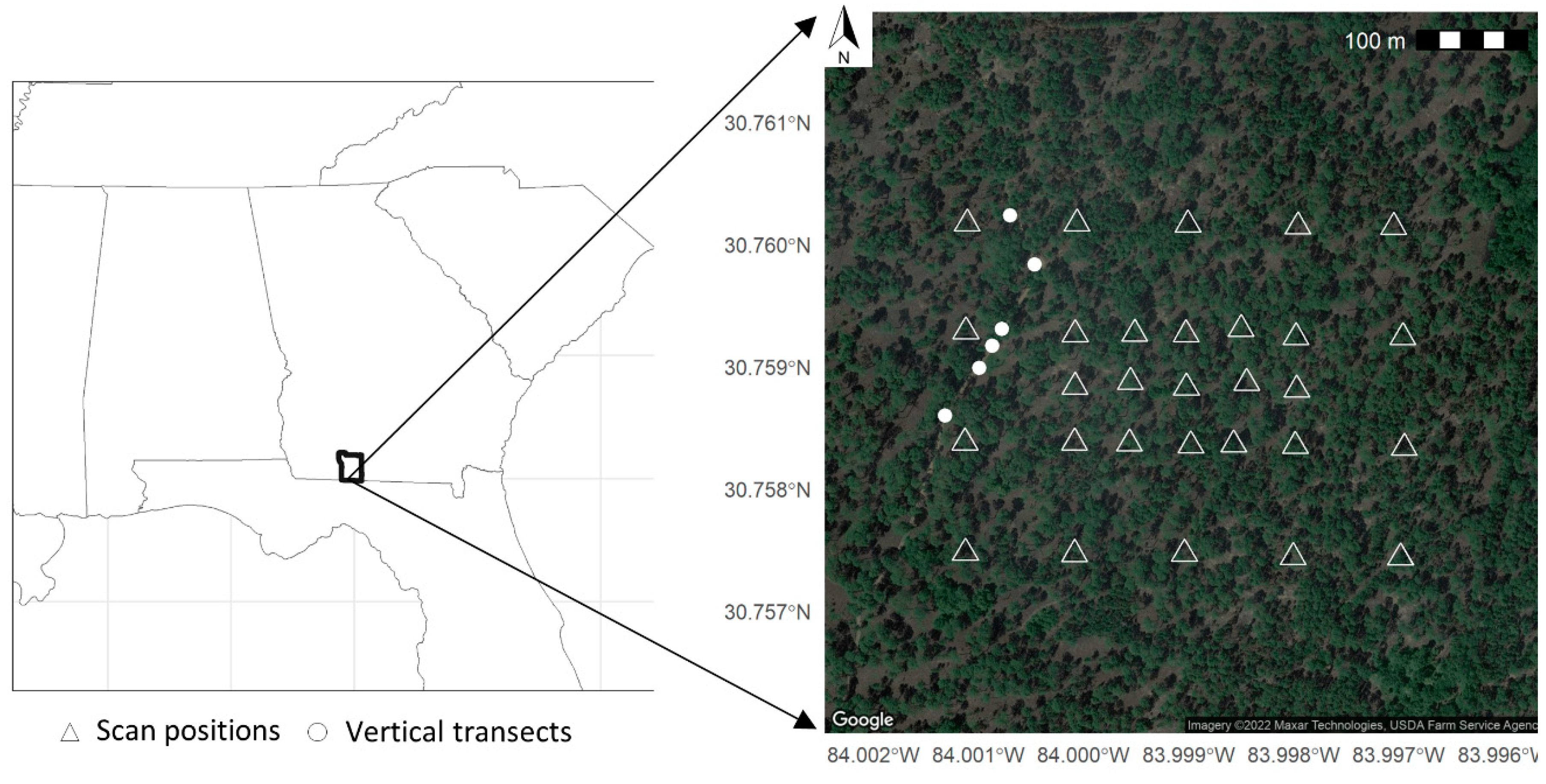
2.1. Site Description

The study site, known as the Wade Tract Preserve (https://talltimbers.org/research-the-wade-tract-preserve/ (Accessed 5 January 2022), is an 85-ha old-growth longleaf pine (Pinus palustris Mill.) stand protected by a conservation easement held by Tall Timbers Land Conservancy on Arcadia Plantation in the Red Hills regions of Thomas County, GA, USA (Figure 1) [34]. Historically, the canopy structure of longleaf pine ecosystems was influenced by frequent disturbance, such as lightning-induced fires, burning by indigenous peoples, and hurricanes [35,36,37]. The formation of relatively large canopy gaps following disturbance events facilitates light transmittance to the forest floor, supporting resource availability and seed recruitment [38,39]. The few-remaining intact ecosystems are often characterized as savannas or woodlands and possess incredibly diverse understories dominated by grasses and forbs, which is facilitated by their open, yet structurally complex canopies [40,41]. The plant community is very diverse—more than 500 native plant species have been documented within the Wade Tract easement. Tree-ring dating from coring has revealed that many of the trees are more than 200 years old, several of which range up to 500 years [42]. While the overstory is dominated by longleaf pine (average basal area 22 m² ha⁻¹), some broadleaf trees are present, mostly oaks (Quercus spp.) and hickory (Carya spp.). The ground cover vegetation is dominated by warm season cespitose grasses (especially Aristida beyrichiana Trinius & Ruprecht, Schizachyrium scoparium (Michaux) Nash, and Sorghastrum secundum (Elliott) Nash). During the past century, the Wade Tract has been managed for northern bobwhite hunting and conservation using frequent (annual/biannual) prescribed fires and there are no records of logging activity.

Climate in the region is classified as humid subtropical [45] with mean monthly temperatures ranging from 27.8 °C in July to 10.7 °C in January and mean annual rainfall of 1380 mm [46]. The soils are dominated by well-drained Ultisols (Typic and Arenic Kandiudults) derived from Pliocene sediments of the Miccosukee Formation and topography is rolling, extending ca. 25–50 m above mean sea level [47]. Frequent (annual/biannual) burning has been conducted on the plantation, including the Wade Tract Preserve, for as long as plantation records exist [46,48].

2.2. Data Collection

2.2.1. Field Data

Field data were collected in July of 2017 along six vertical transects established within the Wade Tract for the purpose of model evaluation (Figure 1). At each transect, DHPs were collected using a Canon EOS Rebel T1i 15.1 MP camera with a 180° fisheye lens and the camera was attached to a tripod. In order to capture DHPs at different heights (Figure 2) above plot center, the tripod mounted camera was attached to a telescopic boom lift [49] at each plot resulting in 24 DHPs in total. A plum bob (i.e., plumline) was used as a vertical reference line to ensure that each hemispherical photo was positioned above plot center. The lens was leveled and oriented towards zenith such that the top of the image corresponds to magnetic north and images were captured before sunset with overcast sky conditions to provide contrast between vegetation and sky. Plot centers were geolocated using a Trimble GEO 7X with a Trimble Zephyr Geodetic antenna set to average 750 points at 50 cm resolution or better and post processed using Trimble TerraSync software (Trimble Inc., Sunnyvale, CA, USA). These points were used to clip ALS and TLS point cloud data to each transect. Because the Wade Tract is a preserve, DHP acquisition with the boom crane was limited to sites along the established road bisecting the old growth stand as to not disturb vegetation and soil.

2.2.2. Airborne Laser Scanning

Discrete-return ALS data were acquired on the 29th of October 2018 using a Leica ALS80 onboard a PA-31 Piper Navajo Chieftain. Flight altitude was 1,280 m aboveground at a speed of ca. 278 km h⁻¹, covering 258 km of total flight line. Laser pulse frequency was 642,800 Hz with a scan rate of 66.1 Hz, obtaining an average point density of 17 ± 3 points m⁻². ALS-data were then processed in R 4.0.3 [50] using the lidR package [51] by first merging returns from individual flight lines and then tiling the data into 1000 m × 1000 m tiles. Duplicate points were removed using the filter_duplicates function, and noise was classified and removed using the IVF (isolated voxels filter) with the classify_noise function. Ground returns were classified using Multilevel B-spline Approximation (MBA) [52,53] with the classify_ground function [51].

2.2.3. Terrestrial Laser Scanning

Terrestrial laser scanning data were collected using a RIEGL VZ-2000 (RIEGL Measurement Systems, Horn, Austria), which has a 100° × 360° field of view, laser pulse repetition rate of up to 1.2 MHz, with a beam divergence (mrad) of 0.3, and maximum resolution of 0.0015°. In total, 29 scans were taken in a 400 m × 800 m subsection of the Wade Tract in July of 2017 (Figure 1). A systematic, geometrical pattern was used for data acquisition of 15 center scans spaced at 50 m while the remaining scans were spaced at 100 m. Scans were registered automatically using RiSCAN Pro 2.8 software and were filtered for noise by first removing returns with a deviation greater than or equal to 14, and/or reflectance values less than or equal to −20. Returns within 2 m or beyond 200 m from the scanner head were removed. Individual scans were merged and duplicate points within a sampling radius of 6 mm were removed. The merged scan was tiled into 100 m × 100 m tiles, resulting in a mean point density of 3827 points m⁻². The individual tiles were further processed in R (4.0.3) [50] using the lidR [51] package. Noise removal and ground classification were performed in the same manner as described for the ALS data.

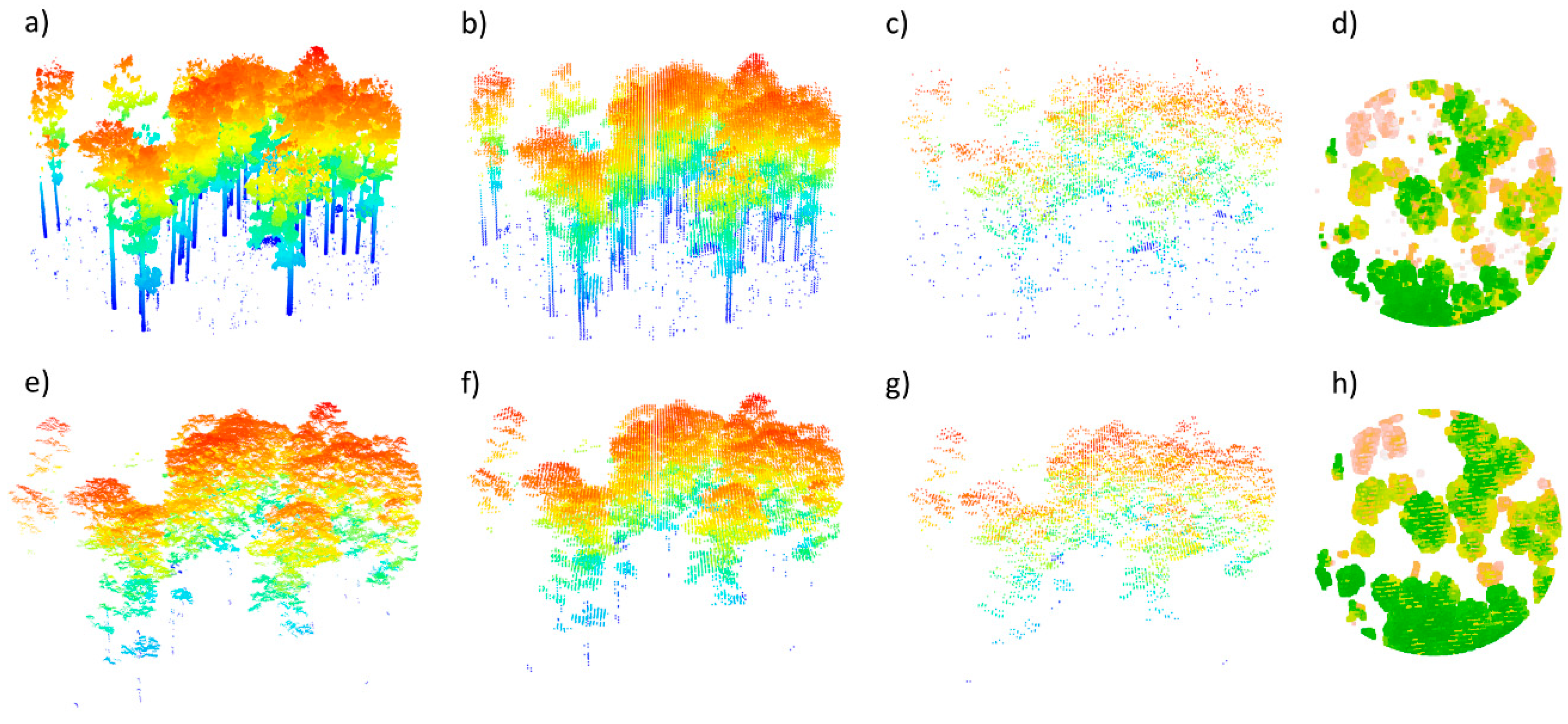
2.3. Point-Cloud Voxelization

LiDAR point-cloud data are often comprised of millions of returns, or echoes, that precisely characterize locations in the X, Y, and Z dimensions, but these returns cannot be used directly to quantify the space occupied by vegetation because points do not have a defined length, width, area, or volume. Additionally, objects that are closer to the LiDAR instrument will be characterized by a higher density of points relative to objects that are further away, resulting in an imbalanced representation of the measured 3D space. A voxel-based technique to overcome the aforementioned challenges is described by Vosselman et al. [25], where the 3D point-cloud space can be divided into a finite number of cubes, or voxels, effectively normalizing the point-density distribution of the LiDAR data. A voxel is the 3D equivalent of a raster cell or pixel, where space is characterized in horizontal and vertical (i.e., X, Y, and Z) dimensions. The positional information of each lidar point determines which voxel that point is contained within, and the metrics describing the LiDAR data are computed from the voxels rather than the individual points. In this analysis, ALS and TLS point-cloud data were voxelized using side lengths of 10, 25, 50, 100, and 200 cm using the voxelize_points function from the lidR package [51]. This allowed the ALS and TLS data to be compared, where each point cloud was transformed into a voxel model indicating the presence of at least one return. Empty voxels, or voxels that did not contain at least 1 return, were omitted from the analysis.

2.4. Estimation of Canopy Gaps

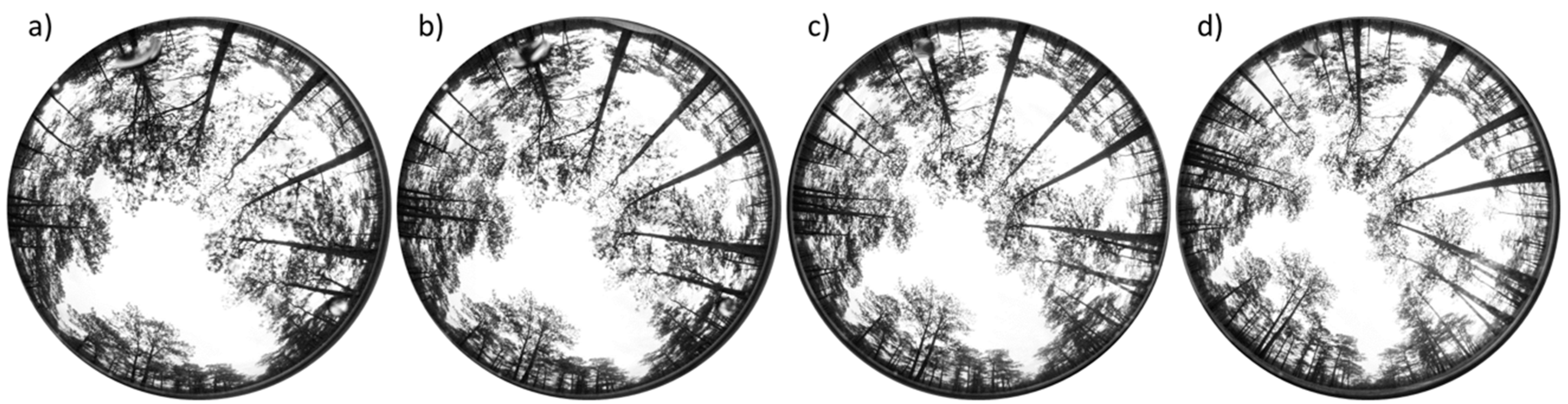
2.4.1. Digital Hemispherical Photography

DHP-derived canopy-gap (CG_DHP) estimates were generated from the WinSCANOPY software [54] by selecting circular rings or zenith annuli at zenith angle range over the entire azimuth angle range (i.e., 0–360°). This approach is suitable for analysis of canopy structure as pixels representing vegetation can be discriminated from pixels representing sky regions, or gaps [27]. Guay et al. [54] define a gap in the canopy—or openness—as the fraction of open sky that is unobstructed by vegetation in the canopy above the lens (three-dimensional space). It accounts for the relative sphere area occupied by each zenith ring. Nine equiangular zenith annuli were defined in the zenith angle range between 0° and 70°, as a result each annulus was 7.8° in width. Canopy gaps were obtained for each annulus by only considering the annulus rings with zenith angles between 0–70°, which helps to remove geometrical distortions that occur with hemispherical lenses at angles greater than 70° [29]. Canopy gaps for a single circular ring (i.e., annulus) located at zenith angle was calculated according to Equation (1).

$$C{G}_{DHP}=\frac{F_s}{F_s+F_v}$$

(1)

where CG_DHP is canopy gap for the annulus centered at θ, F_s is the number of sky pixels in the annulus centered at θ, and F_v is the number of vegetation pixels in the annulus centered at θ.

2.4.2. Voxel-Based Estimates

ALS-derived canopy gaps (CG_ALS) and TLS-derived canopy gaps (CG_TLS) were estimated from the voxelized point-cloud data at each transect by extracting the coordinate (X, Y, and Z) information into a data frame. The Easting (X) and Northing (Y) values were merged into a single column using the “unite” function in the R package dplyr [55]. Voxels with spatially coincident X and Y coordinate values were filtered from the data frame using the dplyr “distinct” function (Figure 3c,g). In other words, voxels that occupied the same Northing and Easting space were removed from the data frame, retaining only voxels with distinct X and Y values. Height (Z) values were then filtered to match the respective height thresholds (1.4, 4, 8, and 12 m) used for DHP-based canopy gap estimates (CG_DHP). For example, point cloud data with z-values ≥1.4 m were compared with hemispherical photographs acquired at 1.4 m aboveground level, while point-cloud data with z-values ≥12 m were compared with hemispherical photographs acquired at 12 m above ground level. Voxel-based canopy gap estimates were derived according to Equation (2).

$$CG=1-\left(\frac{L_v{}^2}{\pi r^2}\right)$$

(2)

where $CG$ is canopy gap, $L_v$ is voxel side length in point cloud units (e.g., 1 m), and $\pi r^2$ is the circular area of the transect with radius $r$ (30 m).

Canopy gap estimates were then scaled-up to the stand-level by applying Equation (2) to 90 randomly selected locations.

2.5. Model Evaluation

LiDAR-derived canopy gap estimates were evaluated against CG_DHP using the Root Mean Squared Error (RMSE, Equation (3)); the square root of the variance of residuals which provides an indication of how close the predicted values (or estimates) match the observations. For the purpose of this analysis, we treated CG_DHP as our observations, while CG_TLS and CG_ALS were considered model estimates.

$$RMSE=\sqrt{\frac{1}{n}{{\displaystyle \sum }}_{i=1}^n{\left(\widehat{y_i}-y_i\right)}^2}$$

(3)

where $y_i$ are the DHP-derived canopy gap estimates, ${\widehat{y}}_i$ are the LiDAR-derived estimates, n is the sample size with i = 1, 2, …, n.

3. Results

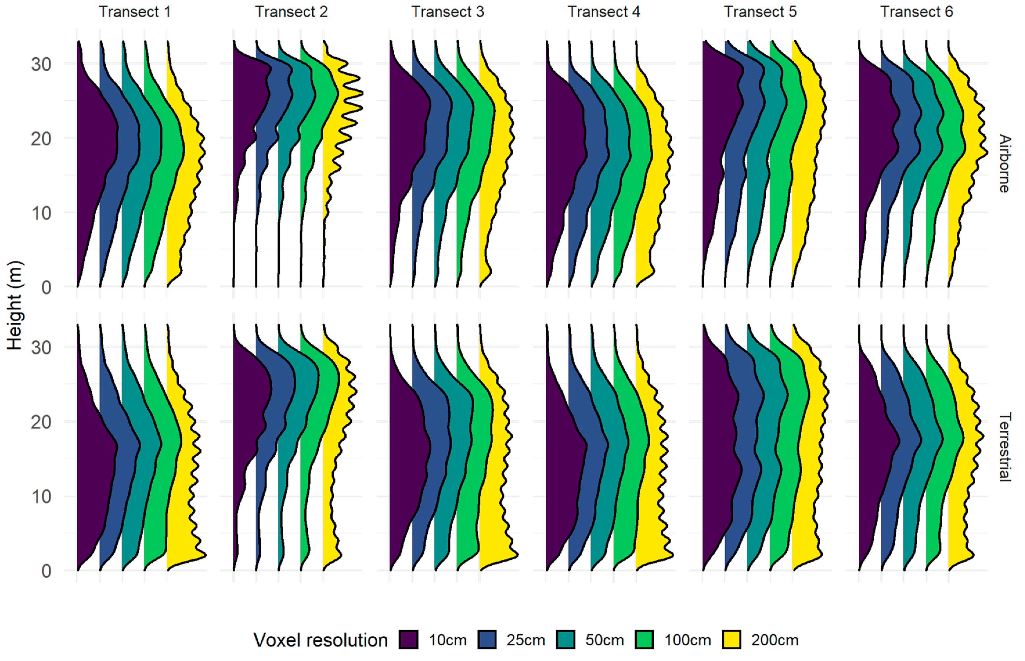
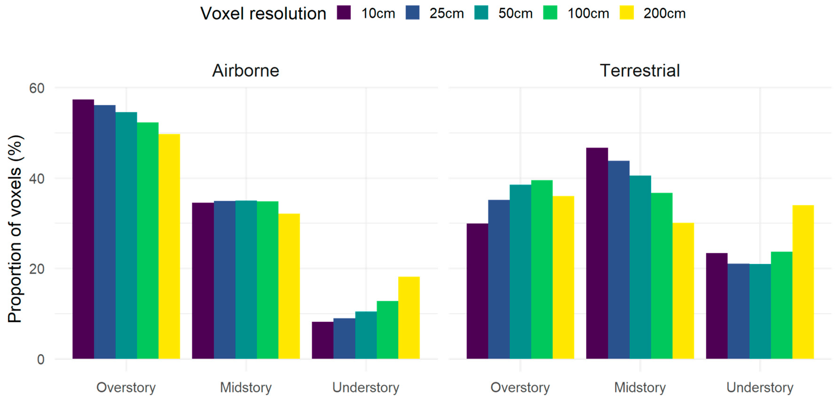
3.1. Point-Cloud Voxelization

Both ALS and TLS point-cloud data were voxelized using five different resolutions. Figure 4 illustrates the probability distribution of LiDAR returns as a function of height for each transect and each platform calculated from the voxelized point-cloud data. The results indicate that the distributions of ALS returns are inversely related to canopy height and that the majority of returns are located in the upper canopy profile. However, the distributions of TLS returns are characterized by a higher degree of between-transect variability. In general, the distributions peak at the midstory layers (10–20 m). However, at Transect 2, for example, the distribution peaks in the canopy layer (>20 m). Comparison of the probability distributions from these two laser-scanning platforms further indicates that the understory vegetation was under sampled by aerial LiDAR due to occlusion from the overstory canopy while terrestrial LiDAR tended to undersample the canopy due to occlusion from the midstory and lower-canopy layers. The best agreement between the overall shape of the probability density estimates occurs at Transect 2 (Figure 2), with the distribution of returns being greatest between ca. 20 and 30 m, which is a strong indication that most of the vegetation at this transect is distributed in the canopy and that the midstory and understory levels are relatively open.

Within-platform variability of the ALS and TLS probability distributions was mostly affected by voxel resolution. With ALS, for example, the overstory contained the largest proportion of voxels irrespective of voxel size. However, the use of increasingly larger voxel sizes affected the vertical profiles by pulling the distribution towards the understory (Figure 5). In other words, as voxel size increased, the proportion of voxels in the overstory decreased while the proportion of voxels in the understory increased. The relationship between voxel size and TLS-derived probability distributions was more nuanced and generally affected the proportion of voxels belonging to midstory rather than the understory. The proportion of voxels in the overstory, for example, increased as voxel size increased from 10–100 cm before decreasing slightly with the use of 200 cm voxels. However, the proportion of voxels associated with the midstory stratum decreased as voxel size increased. These results indicate that the vertical distribution of modeled vegetation is directly affected by the spatial resolution of voxels, which may affect the interpretation and comparison of results among studies.

Resolution also had a dramatic effect on the number of voxels comprising the LiDAR data. Prior to voxelization, the ALS point cloud data ranged from 65.5–102.1 K returns, with an overall mean of 82.2 K when averaged across all six transects. Conversely, the TLS point-cloud data was three orders of magnitude larger on average, ranging from 9.9–30.6 M returns with an overall mean of 18.2 M returns. With 25 cm voxels, for example, the TLS point cloud ranged from 146.1–204.8 K voxels. Conversely, ALS ranged from 48.2–73.1 K voxels when using a 25 cm resolution. Voxelization not only reduced the magnitude of the LiDAR data, but also dramatically reduced file size. With the TLS data, for example, the use of 10 cm voxels reduced the combined file size of all six transects from 1.34 GB to 22.4 MB.

3.2. Plot-Level Canopy Gaps

3.2.1. DHP-Derived Estimates

Our evaluation of CG_DHP indicates that the longleaf-dominated canopies surveyed in this analysis are mostly open but structurally complex, and that this complexity varied considerably within the canopy and across the landscape. As illustrated in Figure 6, canopy gaps and the variability associated with these estimates generally increased with height, ranging from 43–79% across all six transects. The largest range was observed at Transect 4, where CG_DHP increased from 65% at the lowest measurement position (i.e., 1.4 m aboveground) to 78% at the highest measurement position (12 m aboveground). Conversely, the smallest range was observed at Transect 2, where CG_DHP ranged from 59–64%, decreasing as canopy height increased. However, a visual analysis of the binarized images suggests that WinSCANOPY incorrectly identified some of the sky elements at Transect 2 as vegetation at the lower measurement positions, possibly due to changing light conditions and contamination of the image by a small cloud. When averaged across all four measurement positions, mean canopy gap was largest at Transect 3 (74 ± 5%, mean ± one standard deviation) and smallest at Transect 1 (45 ± 2%). The overall average for all transects and all measurement positions was 63 ± 11%.

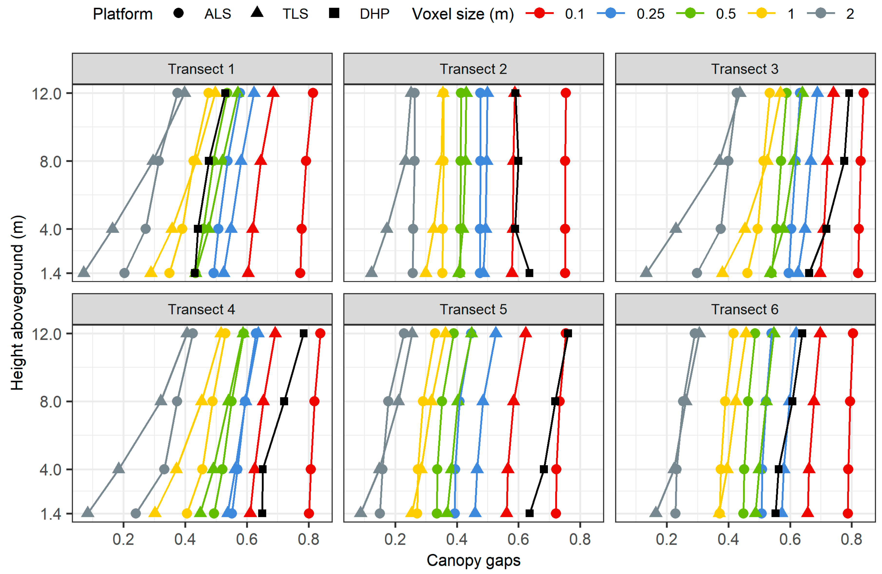
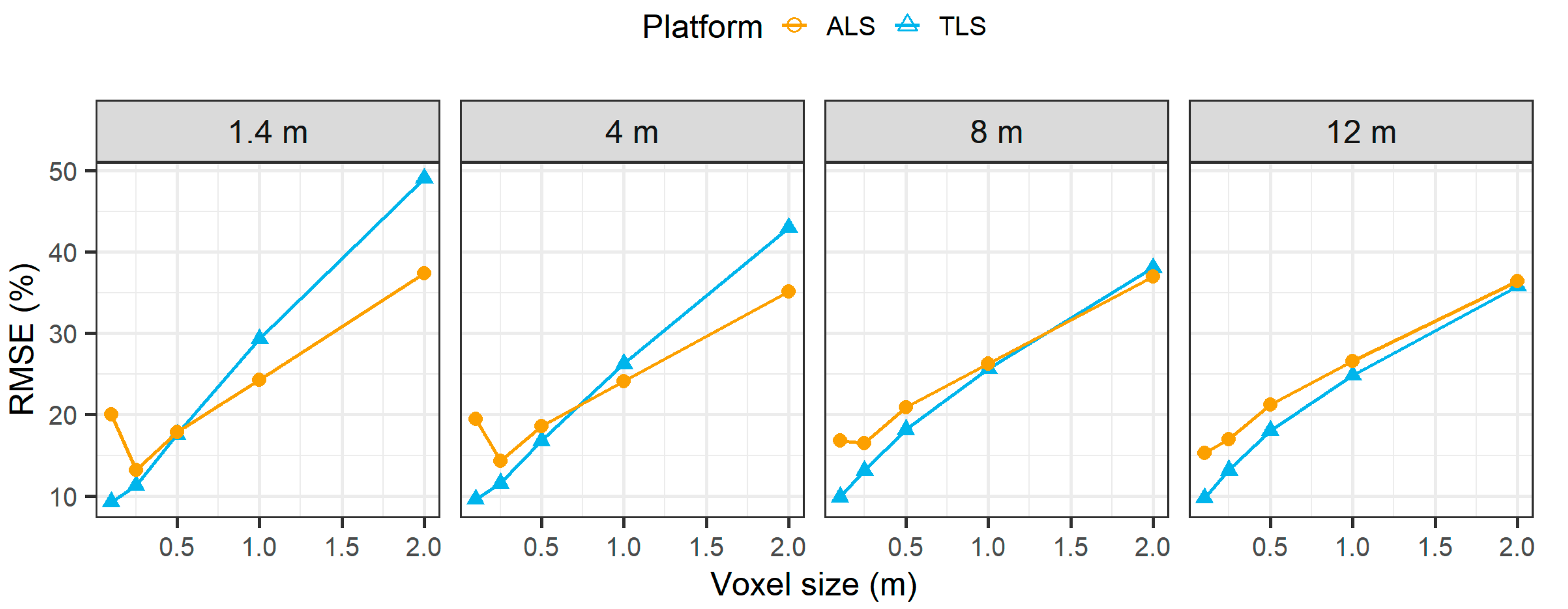
3.2.2. LiDAR-Derived Estimates

LiDAR-derived estimates generally follow the same trend as CG_DHP—canopy gaps increase with canopy height and vary considerably within and between transects. The results from our sensitivity analysis revealed that voxel size had a considerable influence on canopy gap estimation. As illustrated in Figure 7, canopy gap estimates are inversely related to voxel size—smaller voxel sizes yielded larger canopy gaps while larger voxel sizes yielded smaller canopy gaps. Furthermore, LiDAR derived canopy-gap estimates are characterized by relatively large variance both within and between transects and measurement positions.

The best agreement between CG_TLS and CG_DHP was achieved with the use of 10 and 25 cm voxels, which yielded RMSEs of 10% and 12%, respectively. However, the RMSEs were characterized by a large amount of within- and between-transect variation as illustrated in Figure 8. CG_TLS generally agreed well with CG_DHP when using a voxel resolution of 10 cm, and the estimates ranged from 56–74% with an overall mean of 64 ± 5% when averaged across all transects and all canopy height positions. Larger voxel sizes yielded larger RMSEs, which increased from 18–42% as voxel size increased from 50–200 cm. When compared with CG_DHP, for example, the use of 10 cm voxels overestimated canopy gaps by 1% on average, while 25 cm and 200 cm voxels underestimated canopy gaps by 7% and 40%, respectively.

While ALS-derived canopy-gap estimation did not perform as well as terrestrial LiDAR when evaluated against CG_DHP, the overall trends were similar between the two platforms. Smaller voxel sizes again yielded better agreement with CG_DHP; however, the lowest overall RMSE was obtained with 25 cm voxels (15%), followed by 10 cm voxels (18%). For all transects and all canopy heights, 25 cm voxels yielded CG_ALS estimates that ranged from 39–63%, with an overall mean of 52 ± 7%.

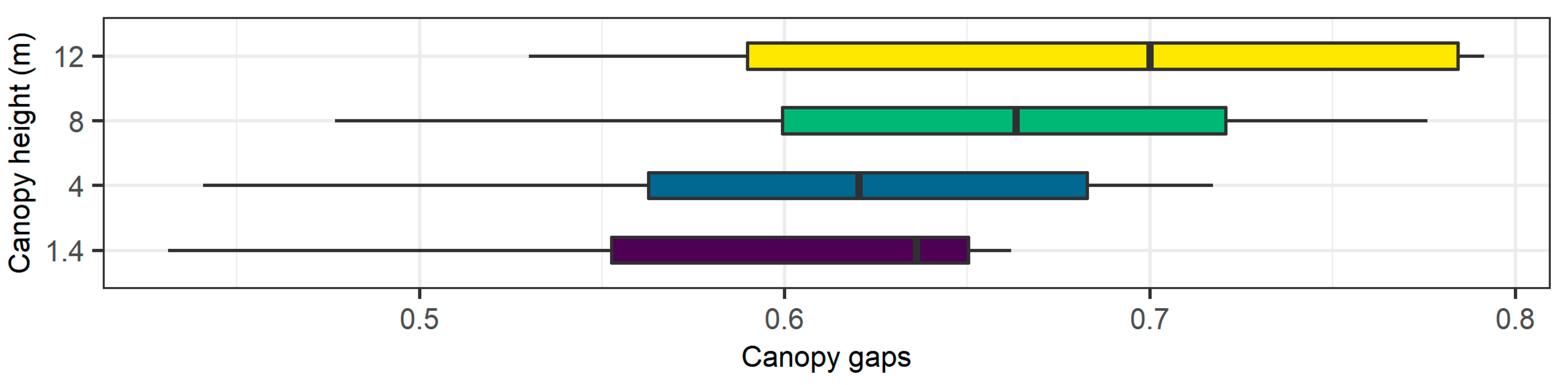
3.3. Stand-Level Canopy Gaps

Upscaling the voxel-based approach across the entire extent of the Wade Tract (0.6 km⁻²) respectively yields canopy gaps that compare favorably with the plot-level estimates. ALS-derived canopy gaps ranged from 68–89% with an overall average of 80 ± 6% with 10 cm voxels, while 25 cm voxels yielded canopy gaps ranging from 25–67% with an overall average of 49 ± 10%. Terrestrial laser scanning was performed in a subsection of the Wade Tract, and therefore has a smaller spatial extent (0.3 km⁻²) relative to the ALS coverage. However, TLS-derived canopy gap estimates are comparable to those derived from ALS when scaled up, and ranged from 32–78% with an overall mean of 52 ± 8% with the use of 0.1 m voxels. Conversely, the use of 25 cm voxels yielded canopy gaps ranging from 23–71% with an overall mean of 44 ± 8%.

4. Discussion

While it is well known that canopy structure governs the spatial and temporal distribution of light transmittance to the forest floor [5,56] relationships between the spatial arrangement of vegetation, and how this vegetation is characterized with 3D models derived from point-clouds, has not been examined extensively. To our knowledge, this analysis represents the first effort for evaluating canopy structure directly from voxelized LiDAR data in longleaf pine ecosystems. We developed a method that circumvents the need to rasterize point-cloud data for input into specialized software designed for digital hemispherical photography. Furthermore, our voxel-based approach provides some key advantages over DHP, including (1) the ability to scale estimates with LiDAR coverage and (2) the ability to sample the study area regardless of lighting conditions, which is often a time constraint with hemispherical photography because images should be acquired before sunrise, after sunset, or under overcast lighting to maximize the contrast between the sky and vegetation.

4.1. Voxel-Size Influence

Identification of an optimal voxel size played a critical role in LiDAR analysis because individual LiDAR returns do not have a defined area or volume, and therefore cannot be used directly to quantify the space occupied by vegetation. Previous research has demonstrated that voxel-size selection represents a compromise among factors including point density, beam diameter, occlusion, and vegetation structure [33,57]. Sampling bias is also introduced due to occlusion, which increases in probability as distance from the scanner increases. Zong et al. [58], for example, reported that denser understory vegetation caused higher rates of occlusion with TLS. Voxel-size also influences occlusion compensation. Generally speaking, smaller voxels have less occlusion compensation relative to larger voxel sizes [32]. For structural assessments such as canopy gap estimation, the voxel size should be small enough to exclude large gaps between branches and crowns, but large enough to characterize regions that are insufficiently sampled by the LiDAR instrument due to low point density and/or occlusion.

The results from our sensitivity analysis indicate that different voxel-sizes yield substantially different canopy gap estimates. As illustrated in Figure 7, canopy gap estimates are inversely related to voxel size. The use of relatively large voxels resulted in a substantial underestimation of canopy gaps, suggesting that voxel sizes of 50 cm and larger did not sufficiently exclude gaps between branches and crowns, resulting in an overestimation of the space occupied by vegetation. The use of 10 cm voxel sizes resulted in an overestimation of canopy gaps with both LiDAR platforms; however, the RMSE and bias were very low with terrestrial LiDAR and generally compared well with the hemispherical photographs. With aerial LiDAR, the lowest overall RMSE and bias was obtained with 25 cm voxels, which suggests that 10 cm voxel sizes were not sufficiently large enough to compensate for occluded regions, and therefore underestimated the space occupied by vegetation.

Our results indicate that 10–25 cm is the optimal size for estimating canopy gaps from voxelized point-cloud data in longleaf pine ecosystems, but estimation agreement with CG_DHP varied considerably with vegetation density, canopy height, and LiDAR platform. These findings generally support those of Zong et al. [58], who determined that the optimal voxel size for TLS-derived visibility estimates was 10 cm in forest plots with low to medium understory cover, but decreased to 5 cm for forest plots with high understory cover. Our results also support the hypothesis of Béland et al. [33], who reported that the optimal voxel size is a function of leaf size, branching structure, and the predominance of occlusion effects, and may range from ca. 5–30 cm. When occlusion effects are negligible, however, Béland et al. [33] postulate that voxel-size selection is mostly related to leaf size. In this analysis, TLS occlusions were minimized by using multiple scanning positions in conjunction with a voxel-based approach, which may explain why TLS-derived estimates had better agreement with hemispherical photography with the use of 10 cm voxels. Conversely, better agreement between ALS and hemispherical photography with 25 cm voxels may be related to occlusion compensation of the midstory and understory stratum.

Voxel resolution also affected the LiDAR-derived canopy gap estimates by altering the probability distributions of the voxelized data. Specifically, larger voxel sizes tended to pull the distribution towards the lower stratum layers (Figure 5). While this affected the vertical distributions derived from each laser-scanning platform, it had a larger effect on TLS-derived canopy gaps at lower canopy heights. For example, the largest overall difference between the LiDAR-derived estimates was observed with the use of 200 cm voxels at a height of 1.4 m (Figure 7). Voxel size, however, did not dramatically affect the relative proportion of the probability distributions. The best agreement between the two platforms, for example, occurs in the midstory canopy layer (Figure 5). These findings suggest that occlusion from the canopy had a larger effect on the ability of ALS to detect vegetation in the lower stratum layers, while occlusion from the midstory layer had a larger effect on the ability of TLS to detect vegetation in the upper canopy.

4.2. Caveats and Considerations

There are several caveats regarding the strength of the assessment results that should be discussed. First, it is important to emphasize that our comparison with CG_DHP is considered an evaluation rather than a true model validation. Although hemispherical photography is widely used in forestry and ecophysiological studies investigating canopy structure and light transmittance at the plot-scale [5,39], the method is sensitive to environmental lighting conditions, exposure settings, the file format used (e.g., JPG vs. raw), and in-camera gamma correction and therefore cannot be considered a proper ground truth [15].

Despite its widespread acceptance in forest gap fraction assessments, directly comparing the two methodologies has some inherent challenges, as the analysis of hemispherical photographs is raster based (e.g., pixel classification), whereas the processing of LiDAR data involves the exploration of patterns and distributions derived from three-dimensional point clouds. Furthermore, hemispherical photography is a passive sensing technique that depends on illumination conditions, whereas active sensors such as LiDAR do not need external sources for illumination of targets. The resulting values are therefore regarded as estimates rather than actual ground truths. As such, the structure of the canopies sampled in this study may be more or less open than the hemispherical photographs suggest. For example, hemispherical images are frequently contaminated by non-uniform sky conditions, resulting in sky elements being misclassified as vegetation. Despite the aforementioned limitations, DHP-derived estimates serve as a useful proxy for model evaluation. Moreover, our results are consistent with similar studies that have reported canopy gaps ranging from ca. 38–85% in longleaf pine [13,59], which provides further confidence in our evaluation of LiDAR-derived estimates.

5. Conclusions

In this analysis, we used voxelized LiDAR data to model the three-dimensional distribution of vegetation structure, from which canopy gaps were calculated to characterize the within-canopy light-environment variability of an open woodland. Proof of concept was demonstrated at six vertical transects, exploring the potential influence of voxel size on canopy gap estimates at the plot scale, without inherent ground sampling bias. Our results indicate that the optimal voxel resolution for canopy gap estimation in open woodlands such as longleaf-pine ranges between 10–25 cm. However, the optimal voxel size varied with LiDAR platform—which may be related to laser penetration and occlusion compensation between the two platforms. Our estimates are characterized by a considerable amount of within- and between-transect variation, which indicates that the horizontal and vertical distribution of vegetation varies considerably within old growth longleaf pine ecosystems, and that the canopy is mostly open but structurally complex. The active vs. passive remote-sensing methodology comparison discussed in this analysis was carried out with the purpose of obtaining a better understanding of the information that can be derived from voxelized LiDAR data and to use that information to develop a method for estimating canopy gaps that scales with LiDAR coverage. The use of vertical transects at each plot allowed us to approximate the three-dimensional nature of canopy structure from hemispherical photography, which is a novel way of quantifying the vertical distribution of canopy gaps as well as the vertical variability associated with these estimates across all three methodologies. Identification of an optimal voxel size is critical for future interpretations of LiDAR data for ecophysiological applications. The ability to leverage findings from this study will allow for a more accurate characterization of the within-canopy light environments, which may in turn explain crown development and other intermediate stand processes [60].

References

1. Gonzalez-Benecke, C.A.; Zhao, D.; Samuelson, L.J.; Martin, T.A.; LeDuc, D.J.; Jack, S.B. Local and General Above-Ground Biomass Functions for Pinus Palustris Trees. Forests 2018, 9, 310. [Google Scholar] [CrossRef] [Green Version]
2. Hudak, A.T.; Bright, B.C.; Pokswinski, S.M.; Loudermilk, E.L.; O’Brien, J.J.; Hornsby, B.S.; Klauberg, C.; Silva, C.A. Mapping Forest Structure and Composition from Low-Density LiDAR for Informed Forest, Fuel, and Fire Management at Eglin Air Force Base, Florida, USA. Can. J. Remote Sens. 2016, 42, 411–427. [Google Scholar] [CrossRef]
3. Ross, C.W.; Hanan, N.P.; Prihodko, L.; Anchang, J.; Ji, W.; Yu, Q. Woody-biomass projections and drivers of change in sub-Saharan Africa. Nat. Clim. Chang. 2021, 1–7. [Google Scholar] [CrossRef]
4. Silva, C.A.; Hudak, A.T.; Vierling, L.A.; Loudermilk, E.L.; O’Brien, J.J.; Hiers, J.K.; Jack, S.B.; Gonzalez-Benecke, C.; Lee, H.; Falkowski, M.J.; et al. Imputation of Individual Longleaf Pine (Pinus palustris Mill.) Tree Attributes from Field and LiDAR Data. Can. J. Remote Sens. 2016, 42, 554–573. [Google Scholar] [CrossRef]
5. Battaglia, M.A.; Mitchell, R.J.; Mou, P.P.; Pecot, S.D. Light Transmittance Estimates in a Longleaf Pine Woodland. For. Sci. 2003, 49, 752–762. [Google Scholar]
6. Gholz, H.L.; Vogel, S.A.; Cropper, W.P.; McKelvey, K.; Ewel, K.C.; Teskey, R.O.; Curran, P.J. Dynamics of Canopy Structure and Light Interception in Pinus Elliottii Stands, North Florida. Ecol. Monogr. 1991, 61, 33–51. [Google Scholar] [CrossRef] [Green Version]
7. Swinehart, D.F. The Beer-Lambert Law. J. Chem. Educ. 1962, 39, 333. [Google Scholar] [CrossRef]
8. Ross, J. The Radiation Regime and Architecture of Plant Stands (Tasks for Vegetation Science); Springer: Dordrecht, The Netherlands, 1981; ISBN 978-90-6193-607-7. [Google Scholar]
9. Hawley, C.M.; Loudermilk, E.L.; Rowell, E.M.; Pokswinski, S. A novel approach to fuel biomass sampling for 3D fuel characterization. MethodsX 2018, 5, 1597–1604. [Google Scholar] [CrossRef]
10. Hiers, J.K.; O’Brien, J.J.; Varner, J.M.; Butler, B.W.; Dickinson, M.; Furman, J.; Gallagher, M.; Godwin, D.; Goodrick, S.L.; Hood, S.M.; et al. Prescribed fire science: The case for a refined research agenda. Fire Ecol. 2020, 16, 1–15. [Google Scholar] [CrossRef] [Green Version]
11. Loudermilk, E.L.; Hiers, J.K.; O’Brien, J.J.; Mitchell, R.J.; Singhania, A.; Fernandez, J.C.; Cropper, W.P.; Slatton, K.C. Ground-based LIDAR: A novel approach to quantify fine-scale fuelbed characteristics. Int. J. Wildland Fire 2009, 18, 676–685. [Google Scholar] [CrossRef] [Green Version]
12. Skowronski, N.S.; Gallagher, M.R.; Warner, T.A. Decomposing the Interactions between Fire Severity and Canopy Fuel Structure Using Multi-Temporal, Active, and Passive Remote Sensing Approaches. Fire 2020, 3, 7. [Google Scholar] [CrossRef] [Green Version]
13. Battaglia, M.A.; Mou, P.; Palik, B.; Mitchell, R.J. The effect of spatially variable overstory on the understory light environment of an open-canopied longleaf pine forest. Can. J. For. Res. 2002, 32, 1984–1991. [Google Scholar] [CrossRef]
14. Evans, G.C.; Coombe, D.E. Hemisperical and Woodland Canopy Photography and the Light Climate. J. Ecol. 1959, 47, 103. [Google Scholar] [CrossRef]
15. Chianucci, F. An overview of in situ digital canopy photography in forestry. Can. J. For. Res. 2019, 227–242. [Google Scholar] [CrossRef]
16. Jonckheere, I.; Nackaerts, K.; Muys, B.; Coppin, P. Assessment of automatic gap fraction estimation of forests from digital hemispherical photography. Agric. For. Meteorol. 2005, 132, 96–114. [Google Scholar] [CrossRef]
17. Beckschäfer, P.; Seidel, D.; Kleinn, C.; Xu, J. On the exposure of hemispherical photographs in forests. iForest—Biogeosci. For. 2013, 6, 228–237. [Google Scholar] [CrossRef] [Green Version]
18. Wagner, S. Calibration of grey values of hemispherical photographs for image analysis. Agric. For. Meteorol. 1998, 90, 103–117. [Google Scholar] [CrossRef]
19. Andersen, H.-E.; Reutebuch, S.E.; McGaughey, R.J. Active Remote Sensing. In Computer Applications in Sustainable Forest Management; Springer: Berlin/Heidelberg, Germany, 2006; pp. 43–66. [Google Scholar]
20. Shan, J.; Toth, C.K. Topographic Laser Ranging and Scanning: Principles and Processing, 2nd ed.; CRC Press: Boca Raton, FL, USA, 2018; ISBN 978-1-315-15438-1. [Google Scholar]
21. Solberg, S. Mapping gap fraction, LAI and defoliation using various ALS penetration variables. Int. J. Remote Sens. 2010, 31, 1227–1244. [Google Scholar] [CrossRef]
22. Lovell, J.L.; Jupp, D.L.B.; Culvenor, D.S.; Coops, N.C. Using airborne and ground-based ranging lidar to measure canopy structure in Australian forests. Can. J. Remote Sens. 2003, 29, 607–622. [Google Scholar] [CrossRef]
23. Lefsky, M.A.; Cohen, W.B.; Acker, S.A.; Parker, G.G.; Spies, T.A.; Harding, D. Lidar Remote Sensing of the Canopy Structure and Biophysical Properties of Douglas-Fir Western Hemlock Forests. Remote Sens. Environ. 1999, 70, 339–361. [Google Scholar] [CrossRef]
24. Hamraz, H.; Contreras, M.A.; Zhang, J. Forest understory trees can be segmented accurately within sufficiently dense airborne laser scanning point clouds. Sci. Rep. 2017, 7, 6770. [Google Scholar] [CrossRef] [PubMed] [Green Version]
25. Vosselman, G.; Gorte, B.G.; Sithole, G.; Rabbani, T. Recognising Structure in Laser Scanner Point Clouds. Int. Arch. Photogramm. Remote Sens. Spat. Inf. Sci. 2004, 46, 33–38. [Google Scholar]
26. Wang, Y.; Fang, H. Estimation of LAI with the LiDAR Technology: A Review. Remote Sens. 2020, 12, 3457. [Google Scholar] [CrossRef]
27. Cifuentes, R.; Van der Zande, D.; Farifteh, J.; Salas, C.; Coppin, P. Effects of voxel size and sampling setup on the estimation of forest canopy gap fraction from terrestrial laser scanning data. Agric. For. Meteorol. 2014, 194, 230–240. [Google Scholar] [CrossRef]
28. Danson, F.M.; Hetherington, D.; Morsdorf, F.; Koetz, B.; Allgower, B. Forest Canopy Gap Fraction From Terrestrial Laser Scanning. IEEE Geosci. Remote Sens. Lett. 2007, 4, 157–160. [Google Scholar] [CrossRef] [Green Version]
29. Zheng, G.; Moskal, L.M.; Kim, S.-H. Retrieval of Effective Leaf Area Index in Heterogeneous Forests with Terrestrial Laser Scanning. IEEE Trans. Geosci. Remote Sens. 2012, 51, 777–786. [Google Scholar] [CrossRef]
30. Takeda, T.; Oguma, H.; Sano, T.; Yone, Y.; Fujinuma, Y. Estimating the plant area density of a Japanese larch (Larix kaempferi Sarg.) plantation using a ground-based laser scanner. Agric. For. Meteorol. 2008, 148, 428–438. [Google Scholar] [CrossRef]
31. Wang, L.; Xu, Y.; Li, Y.; Zhao, Y. Voxel segmentation-based 3D building detection algorithm for airborne LIDAR data. PLoS ONE 2018, 13, e0208996. [Google Scholar] [CrossRef]
32. Lecigne, B.; Delagrange, S.; Messier, C. Exploring trees in three dimensions: VoxR, a novel voxel-based R package dedicated to analysing the complex arrangement of tree crowns. Ann. Bot. 2017, 121, 589–601. [Google Scholar] [CrossRef]
33. Béland, M.; Baldocchi, D.D.; Widlowski, J.-L.; Fournier, R.A.; Verstraete, M. On seeing the wood from the leaves and the role of voxel size in determining leaf area distribution of forests with terrestrial LiDAR. Agric. For. Meteorol. 2014, 184, 82–97. [Google Scholar] [CrossRef]
34. Gilliam, F.S.; Platt, W.J. Effects of long-term fire exclusion on tree species composition and stand structure in an old-growth Pinus palustris (Longleaf pine) forest. Plant Ecol. 1999, 140, 15–26. [Google Scholar] [CrossRef]
35. Fowler, C.; Konopik, E. The History of Fire in the Southern United States. Hum. Ecol. Rev. 2007, 14, 176. [Google Scholar]
36. Loudermilk, E.L.; Cropper, W.P.; Mitchell, R.J.; Lee, H. Longleaf pine (Pinus palustris) and hardwood dynamics in a fire-maintained ecosystem: A simulation approach. Ecol. Model. 2011, 222, 2733–2750. [Google Scholar] [CrossRef]
37. Provencher, L.; Litt, A.R.; Gordon, D.R.; Rodgers, H.L.; Herring, B.J.; Galley, K.E.M.; McAdoo, J.P.; McAdoo, S.J.; Gobris, N.M.; Hardesty, J.L. Restoration Fire and Hurricanes in Longleaf Pine Sandhills. Ecol. Restor. 2001, 19, 92–98. [Google Scholar] [CrossRef]
38. O’Brien, J.J.; Hiers, J.K.; Callaham, M.A.; Mitchell, R.J.; Jack, S.B. Interactions among Overstory Structure, Seedling Life-history Traits, and Fire in Frequently Burned Neotropical Pine Forests. Ambio 2008, 37, 542–547. [Google Scholar] [CrossRef]
39. Palik, B.J.; Mitchell, R.J.; Houseal, G.; Pederson, N. Effects of canopy structure on resource availability and seedling responses in a longleaf pine ecosystem. Can. J. For. Res. 1997, 27, 1458–1464. [Google Scholar] [CrossRef]
40. Jose, S.; Jokela, E.J.; Miller, D.L. (Eds.) The Longleaf Pine Ecosystem. In The Longleaf Pine Ecosystem: Ecology, Silviculture, and Restoration; Springer Series on Environmental Management; Springer: New York, NY, USA, 2006; pp. 3–8. ISBN 978-0-387-30687-2. [Google Scholar]
41. Mitchell, R.; Engstrom, T.; Sharitz, R.R.; De Steven, D.; Hiers, K.; Cooper, R.; Katherine, L. Old Forests and Endangered Woodpeckers: Old-Growth in the Southern Coastal Plain. Nat. Areas J. 2009, 29, 301–310. [Google Scholar] [CrossRef] [Green Version]
42. West, D.C.; Doyle, T.W.; Tharp, M.L.; Beauchamp, J.J.; Platt, W.J.; Downing, D.J. Recent growth increases in old-growth longleaf pine. Can. J. For. Res. 1993, 23, 846–853. [Google Scholar] [CrossRef]
43. Kahle, D.; Wickham, H. ggmap: Spatial Visualization with ggplot2. R J. 2013, 5, 144–161. [Google Scholar] [CrossRef] [Green Version]
44. Walker, K. Tigris: Load Census TIGER/Line Shapefiles; 2021; Available online: https://cran.r-project.org/web/packages/tigris/tigris.pdf (accessed on 31 December 2021).
45. Beck, H.E.; Zimmermann, N.E.; McVicar, T.R.; Vergopolan, N.; Berg, A.; Wood, E.F. Present and future Köppen-Geiger climate classification maps at 1-km resolution, Scientific Data. Nature 2018, 5, 180214. [Google Scholar] [CrossRef] [Green Version]
46. Robertson, K.M.; Platt, W.J.; Faires, C.E. Patchy Fires Promote Regeneration of Longleaf Pine (Pinus palustris Mill.) in Pine Savannas. Forests 2019, 10, 367. [Google Scholar] [CrossRef] [Green Version]
47. Sanders, T. Soil Survey of Leon County; U.S. Department of Agriculture Soil Conservation Service: Leon County, FL, USA, 1981.
48. Glitzenstein, J.S.; Platt, W.J.; Streng, D.R. Effects of Fire Regime and Habitat on Tree Dynamics in North Florida Longleaf Pine Savannas. Ecol. Monogr. 1995, 65, 441–476. [Google Scholar] [CrossRef]
49. Jarvis, R. A Four Wheel Drive Boom Lift Robot for Bush Fire Fighting. In Experimental Robotics: The 10th International Symposium on Experimental Robotics; Khatib, O., Kumar, V., Rus, D., Eds.; Springer Tracts in Advanced Robotics; Springer: Berlin/Heidelberg, Germany, 2008; pp. 245–255. ISBN 978-3-540-77457-0. [Google Scholar]
50. R Core Team R. A Language and Environment for Statistical Computing; R Foundation for Statistical Computing: Vienna, Austria, 2020. [Google Scholar]
51. Roussel, J.-R.; Auty, D.; Coops, N.C.; Tompalski, P.; Goodbody, T.R.; Meador, A.S.; Bourdon, J.-F.; de Boissieu, F.; Achim, A. lidR: An R package for analysis of Airborne Laser Scanning (ALS) data. Remote Sens. Environ. 2020, 251, 112061. [Google Scholar] [CrossRef]
52. Finley, A.; Banerjee, S.; Hjelle, Ø. MBA: Multilevel B-Spline Approximation; 2017; Available online: https://rdrr.io/cran/MBA/ (accessed on 31 December 2021).
53. Lee, S.; Wolberg, G.; Shin, S.Y. Scattered data interpolation with multilevel B-splines. IEEE Trans. Vis. Comput. Graph. 1997, 3, 228–244. [Google Scholar] [CrossRef] [Green Version]
54. Guay, R. WinSCANOPY 2014 for Canopy Analysis; WinSCANOPY Manual Version 2014a; Regent Instruments Inc.: Quebec City, QC, Canada, 2014. [Google Scholar]
55. Wickham, H.; François, R.; Henry, L.; Müller, K. Dplyr: A Grammar of Data Manipulation. 2021; Available online: https://dplyr.tidyverse.org/ (accessed on 31 December 2021).
56. Brockway, D.G.; Outcalt, K.W. Gap-phase regeneration in longleaf pine wiregrass ecosystems. For. Ecol. Manag. 1998, 106, 125–139. [Google Scholar] [CrossRef]
57. Kükenbrink, D.; Schneider, F.D.; Leiterer, R.; Schaepman, M.; Morsdorf, F. Quantification of hidden canopy volume of airborne laser scanning data using a voxel traversal algorithm. Remote Sens. Environ. 2017, 194, 424–436. [Google Scholar] [CrossRef]
58. Zong, X.; Wang, T.; Skidmore, A.K.; Heurich, M. The impact of voxel size, forest type, and understory cover on visibility estimation in forests using terrestrial laser scanning. GIScience Remote Sens. 2021, 58, 323–339. [Google Scholar] [CrossRef]
59. Mitchell, R.J.; Hiers, J.K.; O’Brien, J.J.; Jack, S.B.; Engstrom, R.T. Silviculture that sustains: The nexus between silviculture, frequent prescribed fire, and conservation of biodiversity in longleaf pine forests of the southeastern United States. Can. J. For. Res. 2006, 36, 2724–2736. [Google Scholar] [CrossRef] [Green Version]
60. Franklin, J.F.; Mitchell, R.J.; Palik, B.J. Natural Disturbance and Stand Development Principles for Ecological Forestry; Tech. Rep. NRS-19; Newton Square, PA.; U.S. Department of Agriculture, Forest Service, Northern Research Station: Leon County, FL, USA, 2007; Volume 19, p. 44. [CrossRef] [Green Version]
Figure 1. Location of the study area within Thomas County, GA (inset), terrestrial laser scanning positions (triangles), and digital hemispherical photographs acquired at vertical transects (circles). Satellite imagery was obtained using Google Earth API and the R package ggmap [43], state and county boundaries were obtained from the US Census Bureau using the R package tigris [44].
Remotesensing 14 01054 g001
Figure 2. Example of a vertical stack of hemispherical photographs acquired at Transect 2 using four height thresholds, where (a) corresponds to 12 m aboveground, (b) corresponds to 8 m aboveground, (c) corresponds to 4 m aboveground, and (d) corresponds to 1.4 m aboveground.
Remotesensing 14 01054 g002
Figure 3. Stages of voxel-based canopy gap estimation, where (a) shows the TLS point-cloud data from Transect 1; (b) shows the 25 cm voxelized point cloud data; (c) shows the thinned point cloud, retaining only voxels that occupy distinct X and Y space; and (d) shows a ‘birds-eye’ view of the thinned point cloud. Panels (eh) show the voxel-based canopy gap estimation stages using ALS.
Remotesensing 14 01054 g003
Figure 4. Probability distributions of LiDAR returns as a function of height for each transect and each platform calculated from the voxelized point-cloud data.
Remotesensing 14 01054 g004
Figure 5. The proportion of voxels as a function of forest stratum. The understory and overstory respectively correspond to ≤10 m and ≥20 m height intervals.
Remotesensing 14 01054 g005
Figure 6. Canopy-gap estimates measured using digital hemispherical photography (DHP) in old growth longleaf pine (Pinus palustris). Canopy gaps and the variation associated with these estimates increase as canopy height increases. Estimates were derived from six transects using four measurement positions, or canopy heights, as indicated on the y-axis.
Remotesensing 14 01054 g006
Figure 7. Canopy gap estimates derived from digital hemispherical photography (DHP), airborne laser scanning (ALS), and terrestrial laser scanning (TLS) along the six vertical transects.
Remotesensing 14 01054 g007
Figure 8. Root mean square error (RMSE) of the canopy gap estimates derived from airborne laser scanning (ALS) and terrestrial laser scanning (TLS) for each of the four height thresholds (m aboveground) and each voxel size. ALS and TLS-derived estimates were evaluated against reference values obtained from hemispherical photography.
Remotesensing 14 01054 g008
Publisher’s Note: MDPI stays neutral with regard to jurisdictional claims in published maps and institutional affiliations.