1. Introduction
The invasion of exotic species to any ecosystem can have catastrophic effects when the exotic species outcompete native species and substantially alter landscapes [
1,
2]. Landscape change can lead to significant economic cost [
3,
4]. The invasion of annual grasses in arid and semiarid ecosystems across the globe continues to transform these habitats and alter their biodiversity [
5].
The invasion of large swaths of rangeland ecosystems in the western United States by exotic annual grass (EAG), such as cheatgrass (
Bromus tectorum) and medusahead (
Taeniatherum caput-medusae), have affected wildlife habitat by altering the abundance and diversity of native species. The invasion of the exotic annuals in these rangeland ecosystems have led to increases in wildfire frequency, the spread rate, and intensity by providing a fine-fuel bed as EAG emerge early in the growing season, depriving native plants of critical moisture and nutrients from the soil, and senescing before the hot summer days arrive [
6,
7,
8,
9].
Wildfires in these ecosystems further exacerbate habitat loss by disturbing the land, thus, making restoration difficult and expensive [
10]. The positive feedback mechanism between fire and EAG lead to the expansion of the exotic annuals [
11], further adding to land management costs [
12]. Several studies have successfully created EAG maps at various spatiotemporal resolutions with different temporal latencies over rangeland ecosystems of the western United States [
7,
11,
13,
14,
15,
16,
17,
18].
For example, Rigge et al. [
15] and Jones et al. [
17] covered most of the western United States developing their historical annual herbaceous and annual grass and forb percent cover maps, respectively. However, both studies included native/non-native grass and forb species. On the other hand, Boyte and Wylie [
18] and Pastick et al. [
19] developed expedited EAG maps focusing only exotic annual grass species but for much smaller regions.
Maps that aggregate multiple species and developed with different methods can be insufficient to land managers as each species has its own characteristics and may pose different threats. Moreover, some of the exotic annual species have higher competitive advantages over other exotic annual and native perennial species [
7,
9,
20]. Therefore, species specific maps that cover large spatial extents and are generated with consistent methodologies would provide land managers with a mechanism by which to prioritize land management activities.
Recent advancements in remote-sensing satellite sensors and computational technologies have provided a wide range of newer tools for mapping communities and characteristics of plant species at a range of spatial scales [
13,
16,
17,
21]. Gu et al. [
22] used Moderate Resolution Image Spectroradiometer (MODIS) satellite data, Soil Survey Geographic (SSURGO) productivity data, and regression-tree models and analysis to quantify grassland productivity.
Other studies have used MODIS and regression-tree models to study cheatgrass distributions [
7] or die-off [
20]. Lately, multi-scale satellite sensor approaches have been used to map individual exotic annual species in smaller spatial domains [
9,
16]. Remotely sensed work that supports the early detection, rapid response mapping, and monitoring of exotic annual grass cover by species as well as their phenological confusion with native grass species over regional scales is important for land managers’ understanding of current landscape conditions.
Harmonized Landsat Sentinel-2 (HLS) surface reflectance data provides a useful data source to meet those goals. Pastick et al. [
13,
14,
19] leveraged HLS and machine-learning approaches and demonstrated that EAG could reliably be mapped and monitored with high spatiotemporal resolution. Recently, Weisberg et al. [
23] conducted a phenological analysis and developed species-specific exotic annual grass maps using high-resolution imagery acquired from small, unoccupied aerial vehicles and machine learning to a small spatial extent. They found that each species showed significant differences in seasonal phenology even though they were similar spectrally and spatially during their active growth period.
The primary goal of this research was to explore whether the spatiotemporal and spectral resolution of HLS data allow for mapping and monitoring the fractional cover of a suite of exotic annual and native perennial grass species in the rangelands of the western United States. To accomplish this goal, first, we developed a multi-task learning framework that leverages artificial intelligence/machine learning for the simultaneous estimation of multispectral data and subsequent estimation of the abundance of exotic annual and native perennial grass species. The second objective was to assess the spatiotemporal patterns and drivers of grass abundance and potential mapping confusion between species from field observations, remote-sensing, and climate data. The third objective was to assess the inter-annual variability of the grass species cover compared against the regional weather.
2. Materials and Methods
2.1. Study Area, Remote-Sensing Inputs, and Cleaning Contaminated Pixels
In this study, we enhanced the temporal resolution, latency, and specificity of the U.S. Geological Survey (USGS) Rangeland Exotic Plant Monitoring System [
https://www.sciencebase.gov/catalog/item/5f0ddd6e82ce21d4c4053e17 (accessed date: 15 December 2021) ] to develop and publicly release species-specific maps (30-m spatial resolution) of the abundance of exotic annual (combination of multiple species, cheatgrass, and medusahead) and native perennial (Sandberg bluegrass (
Poa secunda)) grasses across much of the western United States (
Figure 1).
In addition to an expanded spatial and temporal scope of our monitoring area, which was divided into all or parts of 376 mapping units (109.9 × 109.9 km) to coincide with the Military Grid Reference System adopted by HLS [
24], we updated the system by integrating different algorithms, modelling techniques, and spectral data to improve predictions.
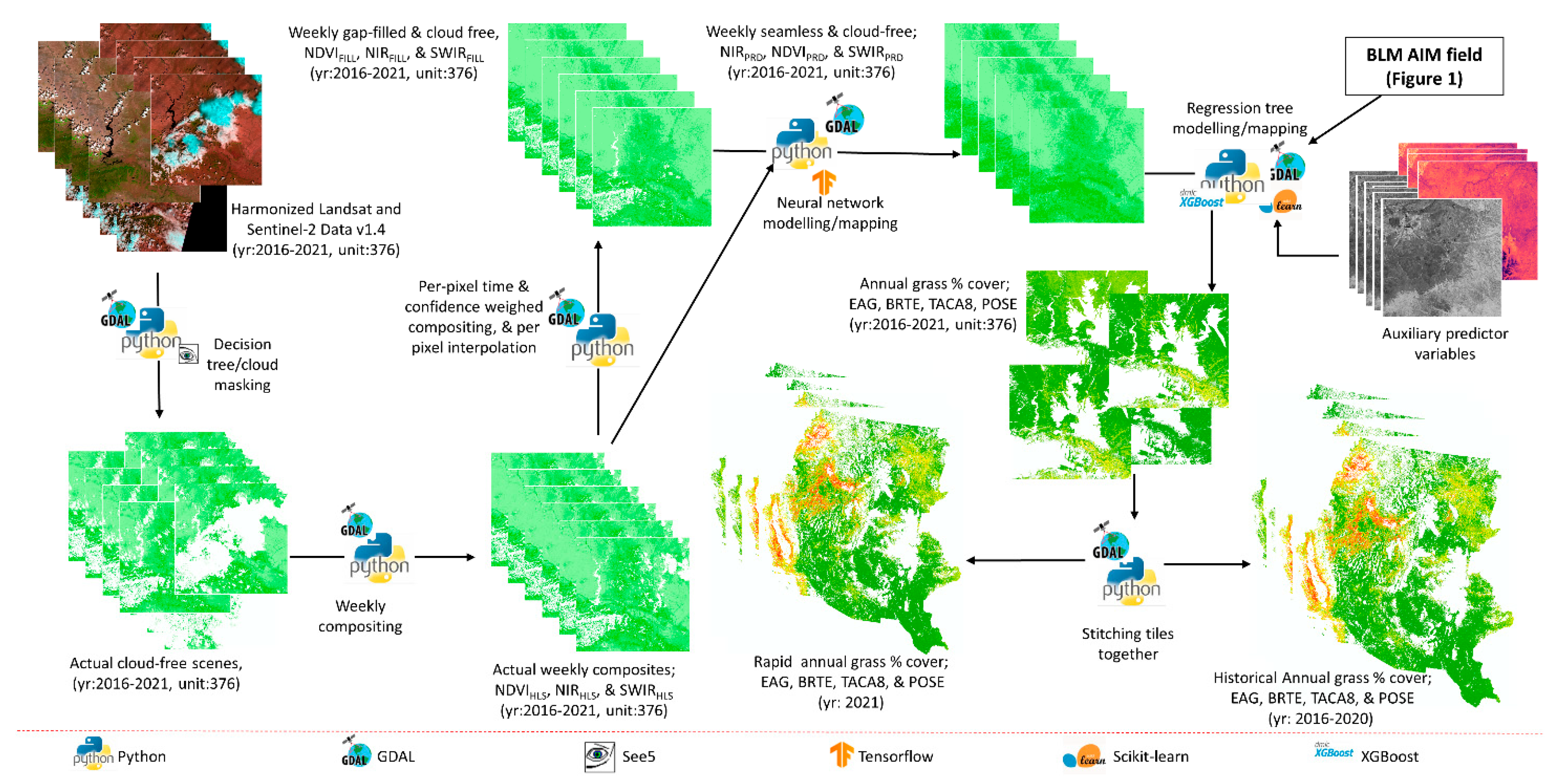
The overall data processing and modelling framework is shown in
Figure 2 and consists of (1) acquiring HLS images and removing cloud/shadow pixels; (2) developing cloud/shadow free weekly spectral layers using a spatiotemporal interpolation approach; and (3) developing species-specific exotic annual and perennial grass percent cover datasets for historical (2016–2020) and rapid (2021) estimation.
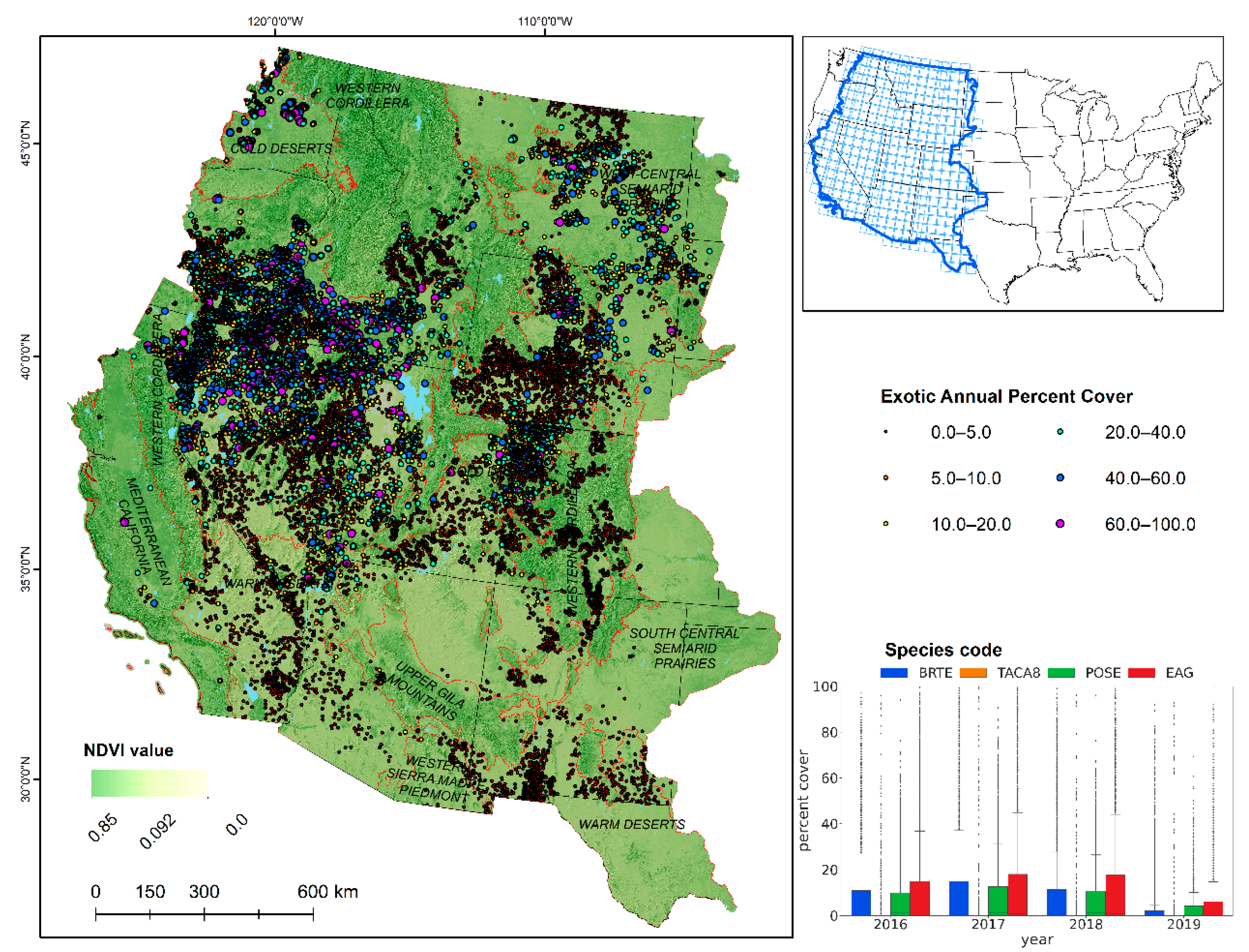
Figure 1.
Field observations of the exotic annual grass abundance overlain on a hillshade model and maximum Normalized Difference Vegetation Index for 2021. Black lines represent state boundaries. Red lines are Omernik Level II ecoregions boundaries [
25], and blue polygons represent permanent terrestrial water bodies. (Inset): 376 individual Harmonized Landsat/Sentinel-2 mapping units overlain with Conterminous United States (upper) and box and whisker plots (lower) showing distribution of selected grass species for training data over the years. The boxes represent interquartile range with horizontal line inside them indicating median values. The whiskers extend to a range that is within the median values ±1.5 times the interquartile range. EAG represents a combination of 16 exotic annuals, BRTE is cheatgrass, TACA8 is medusahead, and POSE is Sandberg bluegrass.
National Aeronautics and Space Administration (NASA) uses surface reflectance data from the Operational Land Imager (OLI) of Landsat satellite and the Multi-Spectral Instrument (MSI) from two Sentinel-2 (A and B) satellites to produce atmospherically corrected land observation data. The multi-sensor feature of HLS data renders a temporal resolution of 2–3 days. We acquired all available HLS (v1.4) 30-m data from the HLS data portal for years 2016–2021.
These data are produced with approximately a 5-day latency period from the satellite observation. More than 298,000 scenes with approximately 23 terabytes of data were acquired for the study, and the complete data processing was conducted on the USGS Tallgrass supercomputer [
26]. We used an automated masking procedure that leveraged HLS imagery and a decision-tree classification model (C5;
https://www.rulequest.com/see5-info.html, accessed on 15 December 2021) because existing HLS (v1.4) QA bands are known to contain omission/commission errors.
Pixels identified as clouds, shadows, and water in the QA bands and with a Normalized Difference Wetness Index (NDWI) ≤0.1 were given a value of 0. Pixels identified as high quality with no contamination except snow/ice, and NDWI values >0.1 were given a value of 1.
Our analysis showed that this threshold resulted in the best shadow and water detection (see Pastick et al. [
14] for details). We further applied a time-series outlier filter to clean the model training data, targeting the omission errors of the HLS QA bands. We filtered out pixels from the QA band where NDWI values exceeded ±25% from the seasonal tile/year NDWI value. For this study, the seasons were defined as day of year <150, 150–190, 190–230, 230–275, >275 giving high priority to the growing season.
Spectral information from five bands (Blue: 0.45–0.51 μm, Red: 0.64–0.67 μm, near infrared (NIR): 0.85–0.88 μm, mid infrared (MIR): 1.57–1.65 μm, shortwave infrared (SWIR): 2.11–2.29 μm) were randomly extracted within five natural breaks clusters of Normalized Difference Vegetation Index (NDVI) for each scene. Decision-tree classification models were calibrated for optimal hyperparameters (i.e., the number of rulesets and boosting trials) using five-fold cross validation and applied to make a binary map with cleaned and contaminated pixels for each scene.
The decision-tree classification framework also resulted in per-pixel estimates of model confidence (hereafter confidence map) as derived from an ensemble of model realizations and the fraction of correctly and incorrectly classified data in each terminal node. The binary maps were used to mask the contaminated pixels from the raw NDVI scenes to produce cleaned raw NDVI.
The cleaned raw NDVI data were aggregated with the confidence map to interpolate missing values in time steps using a time and confidence weighted sum approach [
27]; these data are called gap-filled NDVI. We further generated weekly composites by taking the median values of all the cleaned raw NDVI data, the confidence map, and gap-filled NDVI data. The weekly composite of cleaned raw NDVI (called NDVI
HLS, hereafter) that had higher than 75 percent values in the confidence composite were filtered to select pure pixels.
The pure pixels were further filtered to cover rangeland pixels that were classified as grassland/herbaceous or shrub by 2016 National Land Cover Database [
28]. Up to 2000 pixels per cluster from five natural breaks clusters of these pure pixels of a weekly composite were selected as training samples. The weekly training samples for each mapping unit and year were further aggregated to extract information from all 52 weeks of the weekly composites of gap-filled NDVI (NDVI
FILL), potential annual incident direct radiation (PADR) [
29], and a digital elevation model (DEM) from the National Elevation datasets [
30] of the study area.
These data served as independent (predictor) variables. The NDVI
HLS, NIR
HLS, and SWIR
HLS served as the dependent (outcome) variables for the model. All mapping unit per year datasets were again aggregated to make one training dataset of six years and 376 mapping units with 264 million records. We developed an independent validation dataset using the same approach; however, validation test samples (n = 39.7 million records) were located at least 120 m from the training samples to mitigate spatial correlation that could exaggerate the validation accuracy [
31,
32].
2.2. Time-Series Modelling, Mapping, and Validation of Spectral Data
The USGS Tallgrass supercomputer was used to develop a multivariate deep-learning model for the simultaneous estimation of weekly NDVI, NIR, and SWIR data across our spatiotemporal domain. Predictor variables included (1) weekly NDVI
FILL for all 52 weeks of a year, (2) PADR, (3) elevation, and (4) week of year information. A multi-layer perceptron (MLP) model was developed using TensorFlow [
33] and trained (calibrated) on approximately 264 (26.4) million records that were sampled from clean image composites (i.e., NIR
HLS, SWIR
HLS, and NDVI
HLS) across time and space (see
Section 2.1).
The multi-task, MLP model was trained/calibrated across 50 epochs using Adam’s optimizer (learning rate of 0.001 + reduction on plateaus) and mean standard error (MSE) as a loss function. We deployed drop-out layers and an early-stopping procedure to prevent model overfitting.
The calibrated model was then applied to spatial inputs of the predictor variable within each mapping unit to produce near seamless, weekly composites (NIR
PRD, SWIR
PRD, and NDVI
PRD). A weekly time step of NDWI
PRD data was also computed using NIR
PRD and SWIR
PRD. The multi-task MLP model was validated against the independent test samples (39.7 million) by calculating Pearson’s r, the median absolute error, and the root mean square error. We also compared the weekly NDVI time-series data (NDVI
PRD) to expedited MODIS (eMODIS) NDVI time-series data by generating box and whisker plots. We downscaled smoothed eMODIS at 250-m pixels to 30-m pixels to facilitate the comparison (see Pastick et al. [
13] for the eMODIS smoothing and downscaling process).
2.3. Exotic Annual and Native Perennial Grass Modelling and Mapping
We compiled 17,542 field observations developed by the Bureau of Land Management (BLM) Assessment, Inventory, and Monitoring (AIM) program (i.e., the Landscape Monitoring Framework (LMF) and Terrestrial Aim Database (TerrADat)) from 2016–2019 (
Figure 1). AIM field data were collected with a line-point intercept method [
34,
35] that focused on measuring core terrestrial indicators including plant species cover and composition. The BLM AIM plots were established with random sampling approaches to maintain an unbiased representation of federally managed rangelands.
Indicator variables were collected as 101 pin-drops in two 150-ft intersecting transects (LMF) and typically 150 pin drops in three transects (TerrADat) and aggregated for the plot. We selected data from individual species of interest (
Table 1) and summarized the abundance of (1) a combination of 16 EAGs, (2) cheatgrass, (3) medusahead, and (4) Sandberg bluegrass for model development and validation (
Figure 1). Sandberg bluegrass is a native perennial bunch grass found in much of the western United States and Canada and has phenological traits similar to exotic annual grasses that might lead to mapping confusion [
36].
To permit upscaling of the species abundance data to the entire study area, a suite of predictor variables was selected and input into our machine-learning framework. The first set of predictor variables was made up of spectral phenocurves, which were represented by (1) weekly NDVI
PRD and NDWI
PRD data (
Section 2.2) from weeks of years 1 to 28. NDVI correlates with photosynthetic potential of vegetation and is a widely used spectral index [
22,
37,
38] despite some limitations in dryland ecosystems with low vegetation cover [
39]. The NDWI, on the other hand, correlates the moisture content in vegetation and complements the time step spectral information that was lacking with NDVI [
40]; and (2) two sets of phenometrics (maximum value- MaxN, and week of maximum value- MaxW) were calculated from NDVI
PRD and NDWI
PRD.
The second set of predictor variables were edaphic and included soil organic matter, silt, sand, clay, and available water capacity in the top soil (0–30 cm) [
41]. The third set of predictor variables were 35-years (1985–2019) of climate normals calculated from Daymet climate data for the annual precipitation, annual temperature, summer (June–Sept) months’ temperature, summer months’ precipitation, winter (Oct–May) months’ temperature, and winter months’ precipitation [
42]. The fourth set of predictor variables were the elevation, aspect, slope, and PADR.
The fifth set of predictor variables added vegetation and disturbance context to the model in that we used fractional component estimates of annual herbaceous, perennials herbaceous, and sagebrush from circa 2016 [
43] and long-term spectral change time and change magnitude from Land Change Monitoring, Assessment, and Projection (LCMAP) [
44]. The sixth set of predictor variables added historical (2012–2019) variability of annual grass and forbs [
17] and supplied seed source information to the regression tree model.
The predictor variables were harvested for each field observation plot, coincident with the year of observation, thus, creating a model database. To generate an ensemble of five models, the model database was then randomly split into five subsets. Each subset was used as validation data once, while the remaining four subsets were used to train the model. The process was repeated four times. This ensemble of five sets of boosted regression tree models were developed using python scikit-learn and XGBoost software libraries [
45,
46].
An early stop approach and grid search hyper-parameter optimization method were used to prevent overfitting and identify optimal parameters during each model iteration. This approach utilizes the same set of predictor data to estimate more than one outcome variable, which, in this case, includes three individual species (i.e., cheatgrass, medusahead, and Sandberg bluegrass) and a combination of 16 different EAG species (see
Table 1). Each set of test data was used to validate its corresponding model, and the results were aggregated before reporting.
Each calibrated model was then applied to the spatial input variables to develop maps (30-m pixels) of each variable (EAG, cheatgrass, medusahead, and Sandberg bluegrass), making five maps for each. Median values and variances of the five maps serve as the final annual percent cover maps and confidence level maps of each species for years 2016–2020. While mapping, we applied a mask to areas that were not classified as grassland/herbaceous or shrub by the 2016 National Land Cover Database [
28] and areas above 2250-m elevation to target only likely rangeland ecosystems and areas that are ecologically suitable for the selected species.
Leveraging the historical (2016–2020) model algorithms integrated with up-to-date spectral data for 2021, we developed target species (EAG, cheatgrass, medusahead, and Sandberg’s bluegrass) intra-annual estimated maps in rapid fashion in both May and July for 2021. Here, the long-term average (2016–2020) of the NDVI
PRD was calculated and used as proxy to NDVI
FILL for future 2021 weeks. The MLP model was re-calibrated (
Section 2.2) to estimate a time series of spectral phenocurves (NDVI
PRD, NIR
PRD, and SWIR
PRD) followed by the computation of NDWI
PRD, MaxN, and MaxW for 2021.
We then applied regression tree models to develop rapid annual percent cover maps. The process used in May was repeated in July except we made the spectral datasets current by adding subsequent spectral data to the model so that we could develop more recent estimates of foliar percent cover.
2.4. Assessments of Environmental Drivers and Intra-Species Mapping Confusion
We assessed the importance of predictor variables for estimating the species abundance across each model run using the permutation feature importance method [
30,
47]. We then assessed first-order effects of the top-five predictors on modelled estimates of species abundance using Partial Dependence Plots (PDP), which can show whether the relation between the target species and a variable is linear, monotonic, or more complex [
48] as generated for all five model iterations. The permutation feature importance plots and PDP were developed using matplotlib and ppdbox library in python scikit-learn, respectively.
We assessed intra-species mapping confusion between cheatgrass, medusahead, and Sandberg bluegrass by comparing presence and absence of the species in observed (AIM plots) and predicted data. For this assessment, we identified three sets of AIM plots: all plots with (1) cheatgrass presence, (2) medusahead, and (3) Sandberg bluegrass presence. We evaluated for the presence/absence of one species by the presence/absence of another species, and vice versa, to develop accuracy matrices for the years coincident with the year of observation (AIM plots). For example, in all the plots with cheatgrass presence, we compared how many plots have Sandberg bluegrass or medusahead presence and absence in the observed and predicted data.
2.5. Ecoregion and Trend Analysis
Several studies reported that annual grass abundance/cover positively correlates with the amount of precipitation received annually [
49,
50]. To analyze the effect of annual precipitation to the mapped grass species, we used daily 1-km Daymet precipitation data to calculate an anomaly of a total hydrologic year’s precipitation (previous October to current June) [
41] and compared them to the anomaly of annual average abundance of the grass species for each Omernik ecoregion [
25] within the study area for the years 2016–2021.
3. Results
3.1. Spectral Time-Series Images Modelling, Mapping and Validation
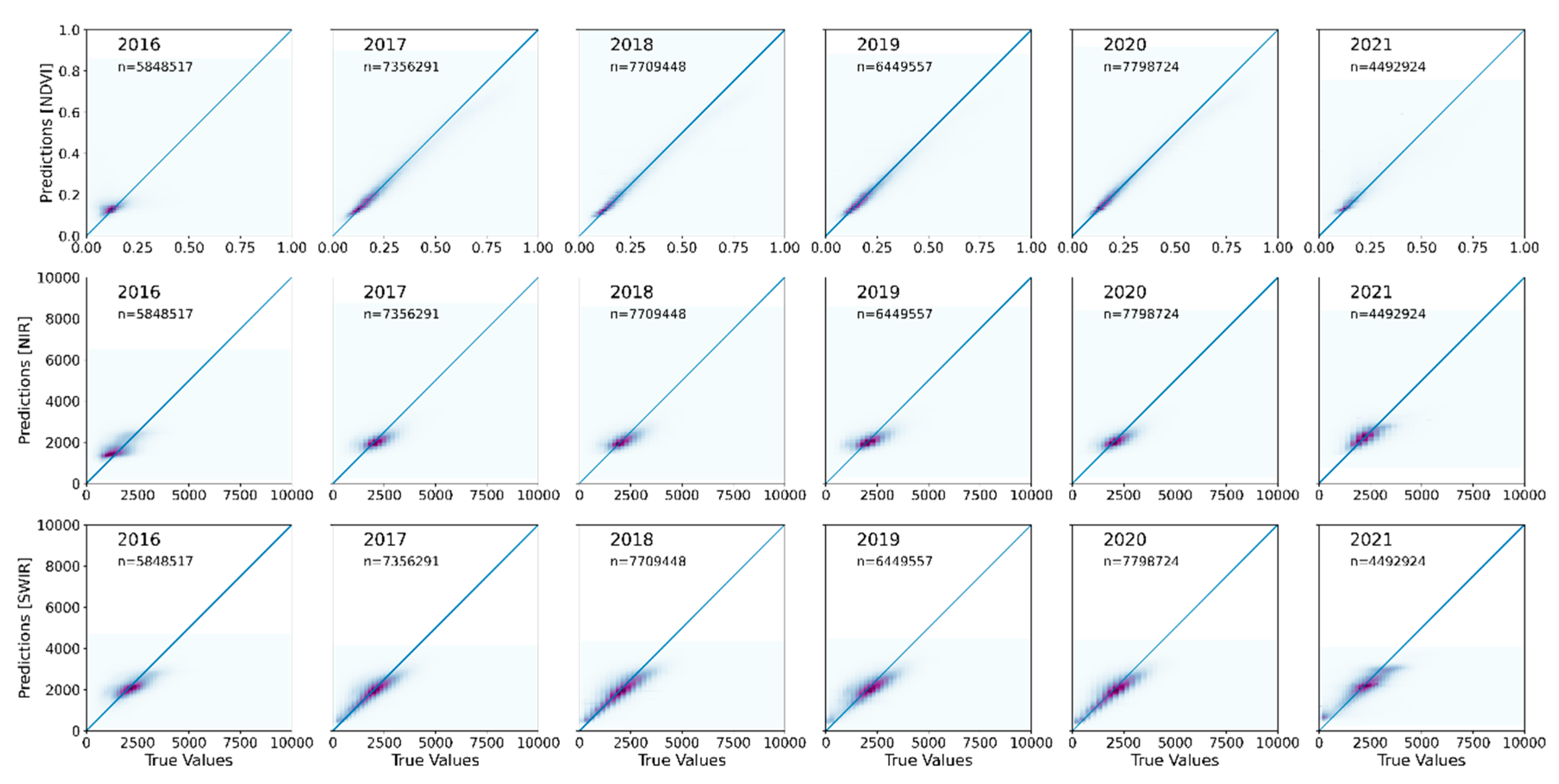
Accurate spectral time-series data are important for developing satellite-based foliar cover products in arid and semiarid rangeland ecosystems, where small differences in inter-annual and inter-seasonal weather patterns can drive larger changes in vegetation productivity. The correlation coefficient of NDVI predictions for all years except for 2016 (0.47) showed strong correlations (0.79–0.95) (
Table 2). Lower data density in 2016 (33,883 satellite scenes) may have contributed to lower accuracy. For comparison, 2018 and 2019 had 66,383 and 71,420 satellite scenes, respectively.
However, despite fewer scenes in 2016, the median absolute error (MdAE) and root mean squared error (RMSE) for NDVI were 0.03 and 0.10, respectively, and within the 2017–2021 range of 0.02–0.04 and 0.08–0.10, (2–10 percent of error). The overall accuracy for NIR (MdAE: about 440–541; and RMSE: about 619–895) and SWIR (MdAE: about 412–498; and RMSE: 556–690) were very similar (4 to 9 percent of error) when compared to NDVI (
Table 2). Predicted values for all independent (test) samples overall were very close to the observed values (
Figure 3), indicating strong correlation.
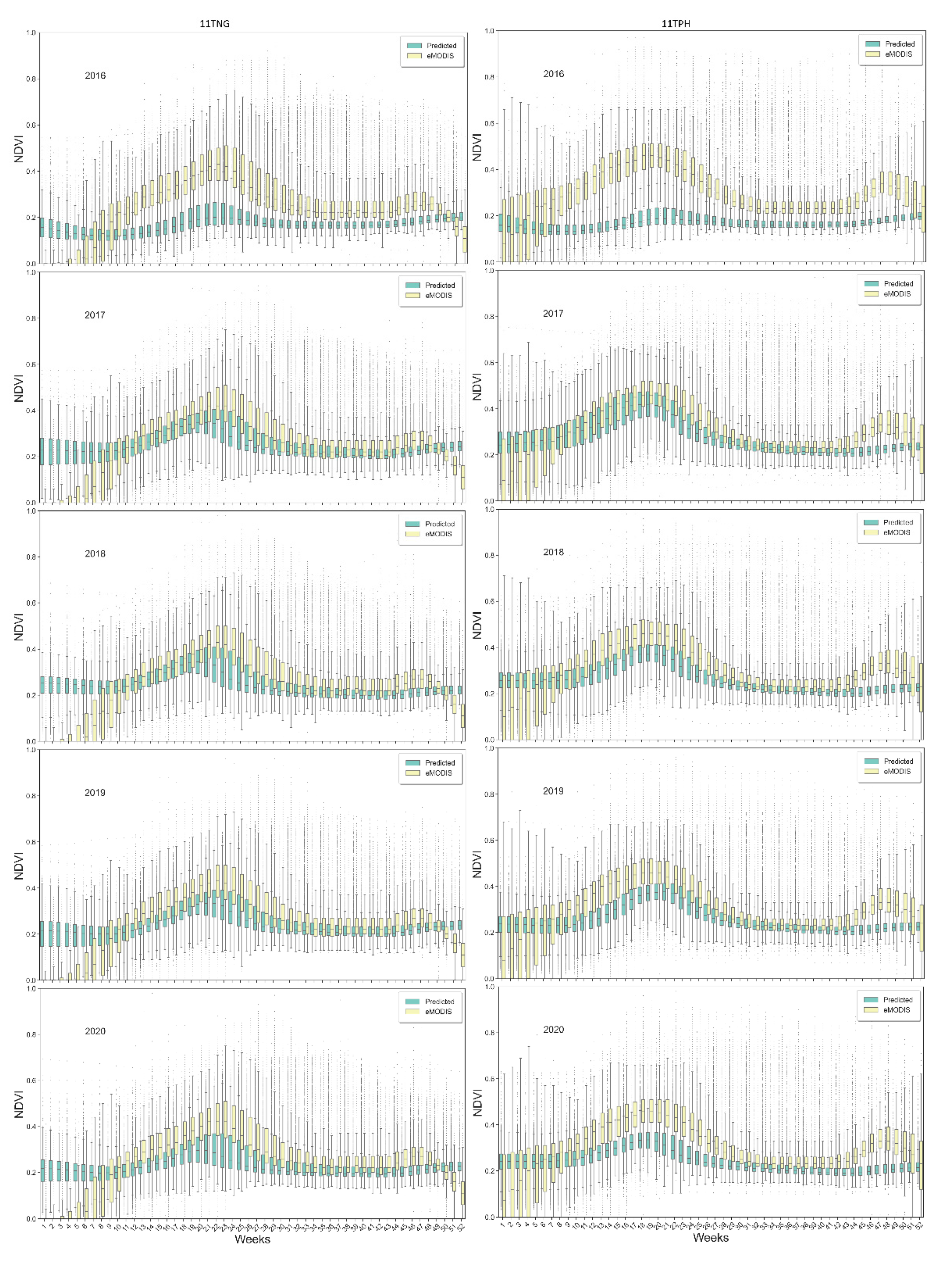
Comparison of NDVI
PRD with eMODIS NDVI time-series revealed our model underpredicted NDVI compared to eMODIS but maintained general agreement between the two datasets for the active growing weeks (box and whisker plots for two tiles as an example in
Appendix A (
Figure A1)). In rangeland ecosystems, vegetation growing conditions are generally favorable in spring, when NDVI
PRD correlates strongly with eMODIS except for 2016.
3.2. Exotic Annuals and Native Perennial Grass Modelling
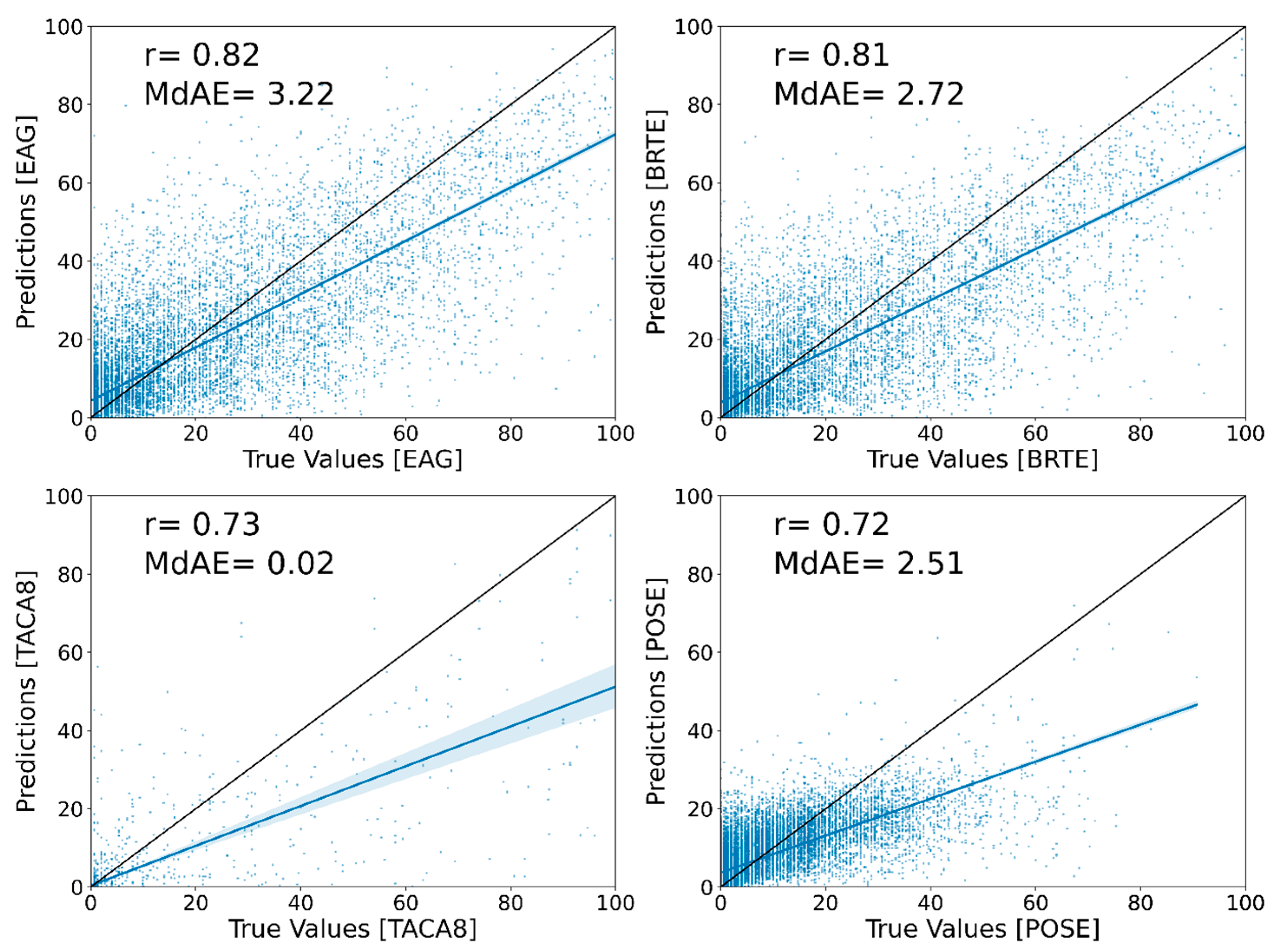
Correlation analysis of independent test values against the predicted values for each species showed general agreement between the two; however, EAG and cheatgrass have higher agreement than medusahead and Sandberg bluegrass (
Figure 4). Overall, the correlation coefficient for EAG is the highest with 0.82, whereas Sandberg bluegrass has the lowest with 0.72. The MdAE for medusahead was excellent with only 0.02 percent error, whereas for EAG, cheatgrass, and Sandberg bluegrass the MdAE values were 3.22, 2.72, and 2.51, respectively.
Medusahead had the smallest training sample size (presence in only 471 AIM plots), compared to others (EAG: 8900, cheatgrass: 7600, and Sandberg bluegrass: 8550), which might have resulted in a higher confidence interval for the modelling.
3.3. Exotic Annuals and Native Perennial Grass Mapping
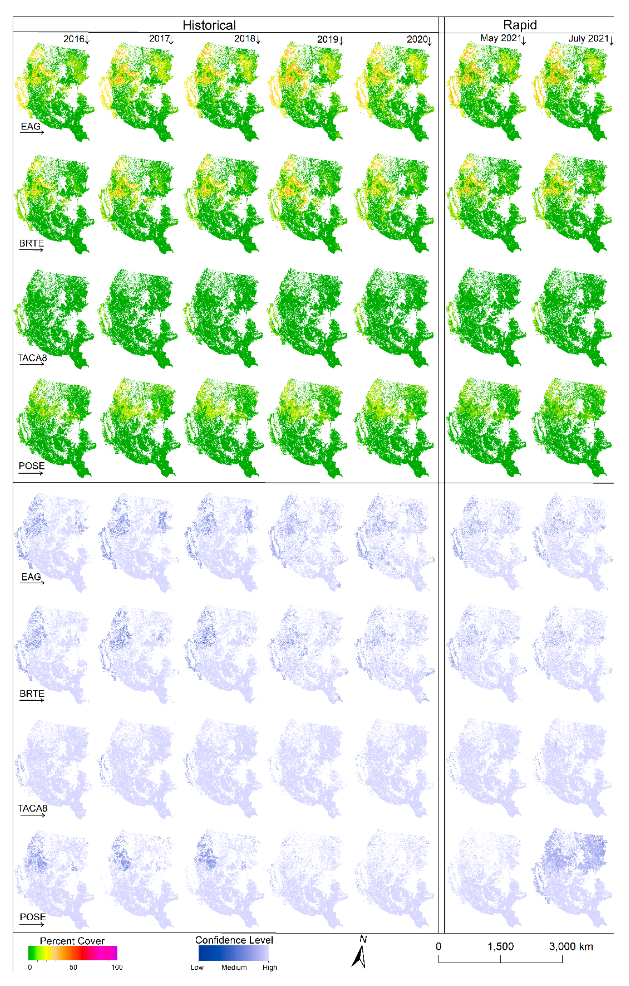
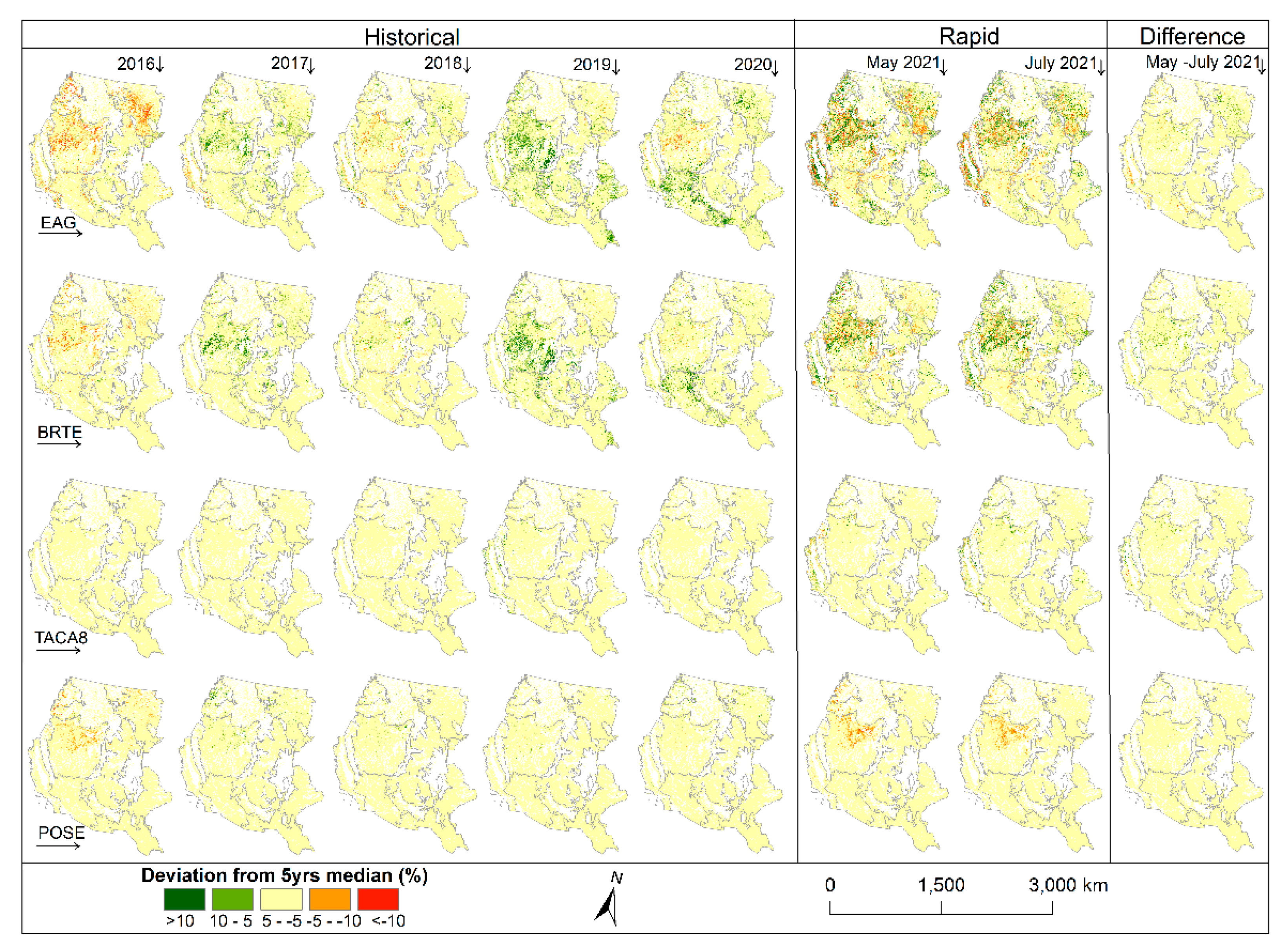
Anomaly and difference maps of species abundance from the long-term (2016–2020) median (
Figure 5; see
Appendix A (
Figure A2) for annual abundance cover with associated confidence maps) provide unique insights into estimated intra and interannual variability. The map for 2016 shows less abundant cheatgrass and EAG in highly invaded areas of the Cold Deserts ecoregion and parts of the West-Central Semiarid Prairies ecoregion with higher abundances for these areas in 2017, 2019, and 2020.
Both versions of the 2021 rapid maps (May and July) predicted variable results for cheatgrass and EAG as the invasion of these grasses was below average in some areas while higher than average in others. Medusahead, which is not wide spread (see
Appendix A (
Figure A2)), appears to have relatively little departure from the long-term median except in 2019, where the Western Cordillera, Mediterranean California, and Great Basin ecoregions show some positive deviation from normal.
The Sandberg bluegrass abundance was less than the long-term median in 2016 but appeared to be more consistent with the long-term median in subsequent years until 2021, when it was substantially less. The Sandberg bluegrass abundance was down on average by 12.4 and 10.4 percent in May and July 2021, respectively, when EAG abundance in the same areas was up on average by 4.7 and 3.2 percent from their respective long-term median.
3.4. Model Drivers and Feature Importance
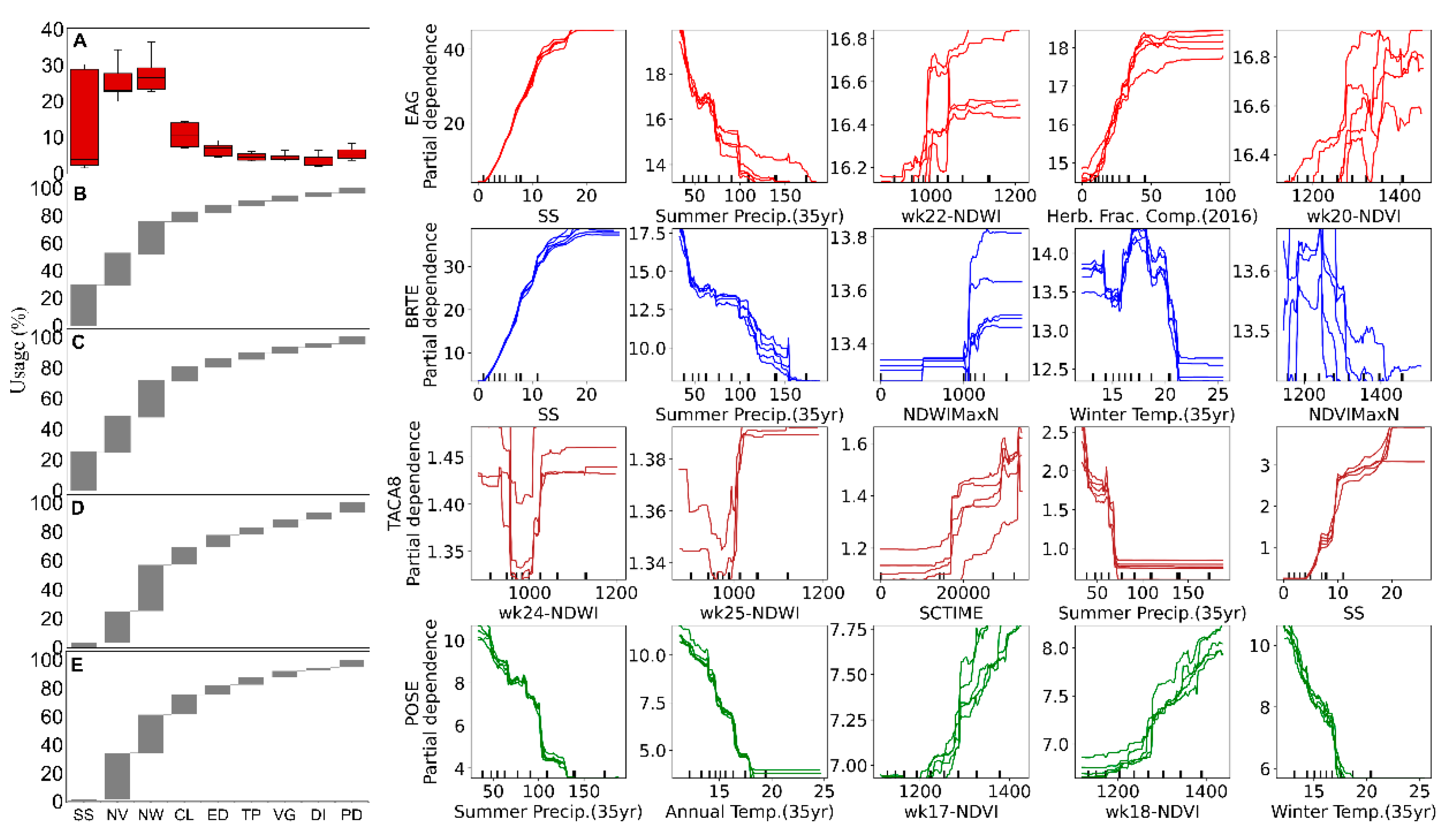
Model-agnostic interpretation methods revealed the feature importance and unique and similar first-order interactions between the estimated grass abundances and environmental predictors (
Figure 6). Model estimates of the EAG abundance and its major constituent cheatgrass cover varied largely as a function of long-term estimates of annual herbaceous cover and variability (proxy for seedbank and invasion envelope) and summer precipitation and, to a lesser degree, as a function of the wetness and productivity indices.
The relation between estimates of EAG abundance and the historical variability of annual herbaceous cover was somewhat sigmoidal with low and high invasion in areas with low and high variability, respectively. Summer precipitation was found to be a useful predictor of species abundances, where cover was generally the highest (lowest) in areas that received relatively less (more) summer rainfall but, by itself, was not highly useful for separating each component.
Targeted species operated in similar climate envelopes, as indicated by similar first-order relations, and observed abundances across similar precipitation and temperature gradients, which indicated that high-order interactions and remote-sensing data largely drove the modeled and mapped differences (
Figure 5 and
Figure 6).
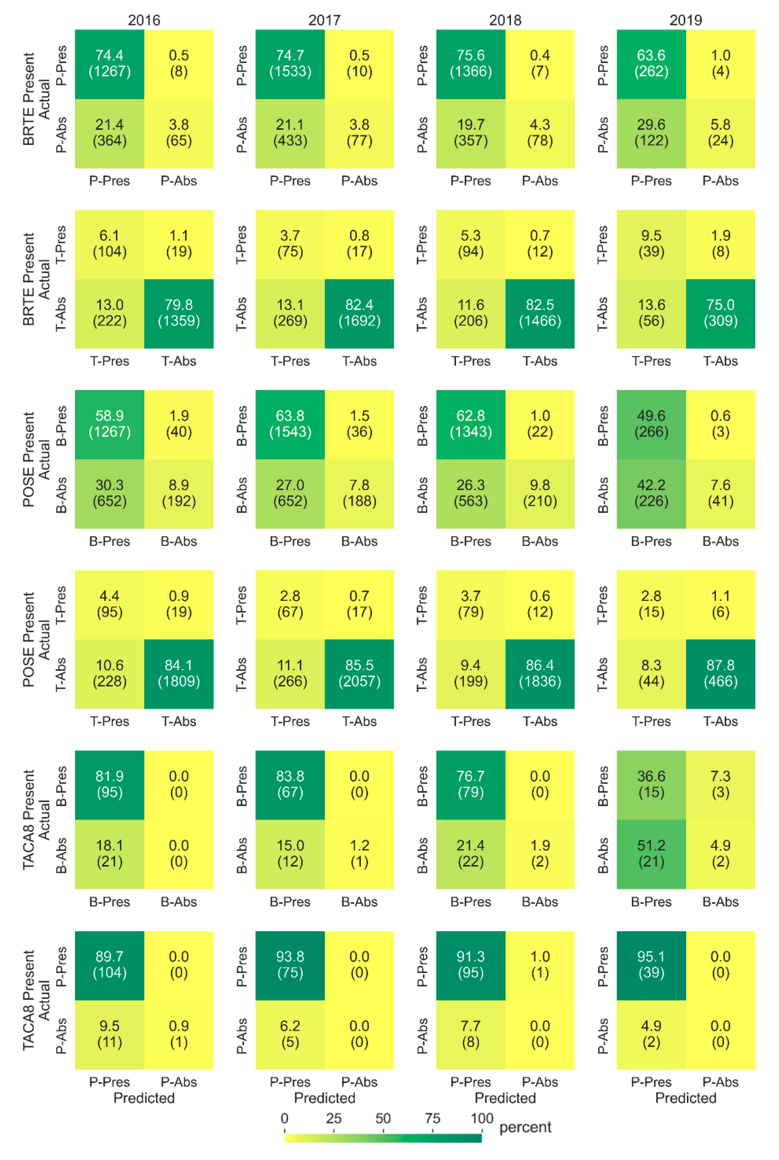
3.5. Intra-Species Mapping Confusion
Our assessment of intra-species mapping confusion between cheatgrass, medusahead, and Sandberg bluegrass found that some confusion existed between the predictions of the species (
Figure 7). Some AIM plots with cheatgrass presence (values > 0) were predicted to contain medusahead (11.6 to 13.6 percent) and Sandberg bluegrass (19.7 to 29.6 percent), when they were not observed on the ground (commission errors).
Overall, the median observed cheatgrass abundance was 17.5 percent in AIM plots with no Sandberg bluegrass, and the models predicted 10.9 percent cheatgrass with 2.2 percent Sandberg bluegrass in those plots (commission errors). Similarly, the median observed cheatgrass abundance was 17.1 percent in AIM plots with no medusahead, and the models predicted 12.4 percent cheatgrass with 0.3 percent medusahead in those plots.
Some AIM plots with Sandberg bluegrass presence (values > 0) were predicted to contain cheatgrass (26.3 to 42.2 percent) and medusahead (8.3 to 11.1 percent) when they were not observed on the ground. Overall, the median observed Sandberg bluegrass abundance, in those presence plots, was 9.1 percent, and the models predicted 8.0 percent with 1.2 percent cheatgrass. Similarly, the median observed Sandberg bluegrass abundance was 9.7 percent in AIM plots with no medusahead and the models predicted 9.0 percent Sandberg bluegrass with 0.2 percent medusahead in those plots (commission errors).
Some AIM plots with medusahead presence (values > 0) were predicted to contain cheatgrass (18.1 to 51.2 percent) and Sandberg bluegrass (4.9 to 9.5 percent) when they were not observed on the ground. However, models rarely missed predicting the grasses (0.0 to 7.3 percent) that AIM plots observed as present (omission errors).
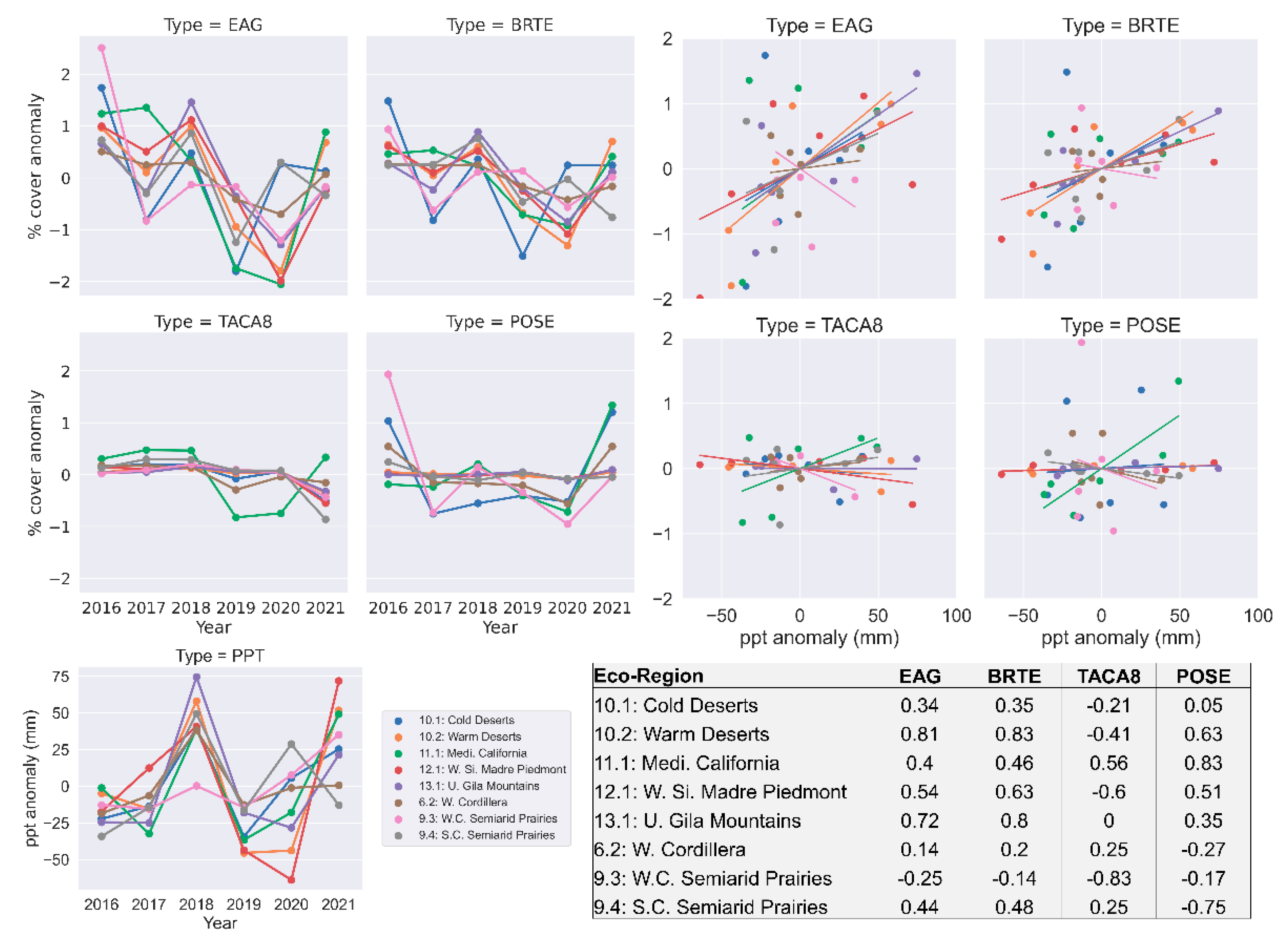
3.6. Inter-Annual Variability of Grass Cover and Relation to Precipitation
The results show that the anomaly of annual averages of cheatgrass (r: 0.46–0.83) and EAG (r: 0.40–0.81) abundances have moderate to high correlations with the anomaly of total hydrologic year precipitation in a majority of the ecoregions. Two ecoregions (Cold Deserts and Western Cordillera) have low correlations, and the West Central Semiarid Prairies ecoregion shows a negative correlation (
Figure 8). The years 2017 and 2019 received the most precipitation for most of the study area. The results show a higher abundance of EAG and cheatgrass for those years. The annual average abundance of medusahead and Sandberg bluegrass shows a relatively weak relation with the annual total precipitation.
4. Discussion
Phenology can be especially dynamic in temperate climates as temperature, precipitation, and other climatic factors vary year-to-year at local scales [
51]. The dynamics become more extreme in arid/semiarid landscapes where precipitation can be the strongest driver of vegetation growth and productivity [
52]. Moreover, plant phenology can be influenced by other factors, such as the elevation, habitat type, and soil type, and can vary pixel to pixel for even the same grass species, especially in arid/semiarid landscapes [
23,
53].
The data fusion approach we implemented to leverage HLS data and machine-learning techniques to develop near-seamless, weekly NDVI proved effective in the arid/semiarid study area [
14,
19]. In this study, we demonstrated the robustness of the approach by expanding the spatiotemporal extent and developing similar quality products for spectral bands, i.e., NIR, and SWIR. We extended the temporal dimension to cover the entire year (52 weeks;
Appendix A (
Figure A2) and increased the spatial extent by approximately three times to cover most of the western United States (
Figure 1).
The implementation of deep learning, neural network algorithms in this study enabled the predictive model to distinguish between phenological differences from coastal climates to desert climates to semi-arid prairies’ climates. However, it is worth noting that this approach requires an enormous amount of training data (264 million records in this study to develop NIR
PRD, SWIR
PRD, and NDVI
PRD; see
Section 2.1) and computational capability. Zhu et al. [
54] reported that a minimum number of training samples is needed to optimize the model accuracy.
We postulate that spatially and temporally balanced training data are equally important for achieving optimal accuracy. Year 2016 had the lowest number of available HLS scenes as Sentinel-2B was not launched until 7 March 2017. This meant that 2016 had about half the scenes of other years, and 2016 had the lowest accuracy in both the imagery processing and EAG predictions by a relatively wide margin (see
Section 3.1).
Predictor variables drive the predictive capability of a model. The more closely a predictor variable represents the characteristics of an outcome variable, the more accurate the modelling outcome. For remote-sensing-based annual grass abundance modelling and mapping studies, satellite spectral bands or spectral band-derived indices are often supplemented by auxiliary variables. Some studies rely on single-date satellite imagery [
9,
55], other studies used two or more dates [
7,
11], and some used time-series data [
14,
19,
23,
49].
However, these studies relied heavily on NDVI to drive model development. NDWI, which is highly sensitive to water content in grassland vegetation [
56], responds quickly to growing grasses, and can improve the modelling accuracy. Our study revealed that NDWI time-series data were similarly influential as NDVI time-series data when driving the model development (
Figure 6).
Similarly, a seed source layer, the variance of annual grass and forb percent cover for 2012–2019 from Jones et al. [
17] as a proxy, was included as a model driver, anticipating that it would improve the accuracy of exotic annual grasses (EAG, cheatgrass, and medusahead). The higher usage of the layer by EAG and cheatgrass and lower usage by Sandberg bluegrass (a perennial grass) in the predicting models met our expectations.
While the functional relations for the estimated medusahead cover followed those of other grass species, the comparatively smaller footprint and fewer training points within areas of high abundance likely resulted in smaller usage of the seed source layer. Further investigation may be needed to better understand these dynamics and identify various stages of medusahead invasion. Future studies that include perennial grass abundance may also benefit by adding the perennial seed source.
Within season (May and July 2021) estimates of EAG and cheatgrass cover growth generally followed temperature gradients as expected, with new growth in ecoregions with later growing seasons (i.e., high latitudes) and slight gains or declines in lower latitudes with earlier starts to the growing season (
Figure 5). Slight declines in the foliar cover from May to July could be effects of grazing or human-induced factors; however, additional investigation would be needed to make that connection.
Stark differences in early season estimates of EAG cover (2021) from the historical average annual cover highlights the effect of weather, and thus spectral data, in estimating cover and dynamic growth patterns of each vegetation component. The substantial loss of Sandberg bluegrass in 2021 from the historical average could be attributed to the increased abundance of EAG as both May and July version of maps estimated higher cover for EAG and lower cover for Sandberg bluegrass than their respective long-term median.
Estimates of the annual abundance of each grass species and their associations with environmental conditions generally aligned with distribution maps and habitat suitability analyses of McMahon et al. [
57]. In their analysis, climate variables were the best predictors of most species’ distribution; however, in this study remote-sensing data were generally more informative for estimating abundance levels. That is, climate data serve as a tool for identifying where species operate but less so for establishing absolute measures of foliar cover.
Although our primary purpose was to map the EAG percent cover, we demonstrated that our modelling approach can also effectively map a native perennial species along with specific EAG species for a large regional area. In this study, we developed both a predictive map of a collection of 16 EAGs and stand-alone predictive maps for cheatgrass, medusahead, and Sandberg bluegrass (
Figure 5 and
Appendix A (
Figure A2)).
Peterson [
11] reported that Sandberg bluegrass, which has similar phenology timings during active growth to cheatgrass (cheatgrass and medusahead including many exotic annuals may have the similar phonology) may have caused a higher estimation of cheatgrass abundance in some part of his study.
Our study shows a similar outcome in about 25% and 10% of the sampled plots for cheatgrass and medusahead, respectively. However, the predicted cover for incorrectly predicted species was substantially smaller than the observed species. The models almost always predicted the species presence when training data (AIM) observed the species as present. Conversely to McMahon et al. [
57], our models were more likely to predict presence in areas where none was observed (i.e., a commission error). Our study reveals that there was a greater level of confusion of cheatgrass between medusahead and Sandberg bluegrass than between medusahead and Sandberg bluegrass (
Figure 7).
The total hydrological year precipitation was positively correlated to the EAG production, whereas native grass production increased when prior years were dry [
8,
58]. Our analysis found a similar outcome between the precipitation and abundances of EAG and cheatgrass where they showed some correlation with the total hydrological year precipitation in the most of our study area except for one ecoregion. The hydrological year precipitation showed no relations with the medusahead and Sandberg bluegrass abundance. (
Figure 8).
Future efforts could focus on identifying the inconsistent relation between the medusahead abundance to the total hydrological precipitation and negative relation of the EAG and cheatgrass abundance to the total hydrological precipitation in West Central Semiarid Prairie ecoregion. However, our results demonstrated that the cheatgrass invasion was high in primarily Sandberg bluegrass’s ecological landscapes (
Appendix A (
Figure A2)); however, these two species demonstrate different relations to the total amount of hydrological year precipitation (
Figure 8).
Previous studies found that areas with cheatgrass have altered soil environments as well as changed nutrient cycling, microbial communities, and soil structure, all of which had lingering effects even after the invasion was removed, making native species, such as Sandberg bluegrass, less competitive in a changing environment [
59,
60,
61]. Other studies found smaller plant size, earlier phenology, and changing root characteristics of perennial grasses in cheatgrass invaded areas [
62,
63].
Thus, the annual amount of precipitation alone may not be sufficient to explain why the Sandberg bluegrass abundance did not show correlation with the annual amount of precipitation. Future studies may benefit by taking account of the changing environment after invasion of exotic annuals in the analysis as well as modelling process along with the weather variables, such as precipitation. The inclusion of weather variables hinges on the availability of data with finer spatial resolution and shorter temporal latency.
In comparison to the earliest version of U.S. Geological Survey Rangeland Exotic Plant Monitoring System, the current approach made it possible to estimate the foliar cover for multiple grass species. The current approach with new algorithms and usage of the USGS Tallgrass supercomputer reduced the total computational time from more than two weeks to less than a week even after expanding the study area by approximately three fold.
The modelling accuracy improved significantly with the current approach (testing r = 0.82 for EAG) compared to the earlier approach (r= 0.72 for EAG) [
19]. However, the current approach used a higher number of predictor variables (84 compared to 36 in the previous version), hence, resulting in more complex regression tree models. It would be beneficial to simplify the model with fewer or a different set of predictor variables without losing the accuracy.


 ,
, 
