Article

Integrating Multi-Source Remote Sensing to Assess Forest Aboveground Biomass in the Khingan Mountains of North-Eastern China Using Machine-Learning Algorithms

1
State Key Laboratory of Tibetan Plateau Earth System and Resources Environment (TPESRE), Institute of Tibetan Plateau Research, Chinese Academy of Sciences, Beijing 100101, China
2
State Key Laboratory of Remote Sensing Science, Aerospace Information Research Institute, Chinese Academy of Sciences, Beijing 100101, China
3
College of Geography and Ocean Sciences, Yanbian University, Yanji 133002, China
*
Author to whom correspondence should be addressed.
These authors contributed equally to this work.
Remote Sens. 2022, 14(4), 1039; https://doi.org/10.3390/rs14041039
Submission received: 14 January 2022 / Revised: 15 February 2022 / Accepted: 18 February 2022 / Published: 21 February 2022

Abstract

:
Forest aboveground biomass (AGB) is of great significance since it represents large carbon storage and may reduce global climate change. However, there are still considerable uncertainties in forest AGB estimates, especially in rugged regions, due to the lack of effective algorithms to remove the effects of topography and the lack of comprehensive comparisons of methods used for estimation. Here, we systematically compare the performance of three sources of remote sensing data used in forest AGB estimation, along with three machine-learning algorithms using extensive field measurements (N = 1058) made in the Khingan Mountains of north-eastern China in 2008. The datasets used were obtained from the LiDAR-based Geoscience Laser Altimeter System onboard the Ice, Cloud, and land Elevation satellite (ICESat/GLAS), the optical-based Moderate Resolution Imaging Spectroradiometer (MODIS), and the SAR-based Advanced Land Observing Satellite (ALOS) Phased Array type L-band Synthetic Aperture Radar (PALSAR). We show that terrain correction is effective for this mountainous study region and that the combination of terrain-corrected GLAS and PALSAR features with Random Forest regression produces the best results at the plot scale. Including further MODIS-based features added little power for prediction. Based upon the parsimonious data source combination, we created a map of AGB circa 2008 and its uncertainty, which yields a coefficient of determination (R2) of 0.82 and a root mean squared error of 16.84 Mg ha−1 when validated with field data. Forest AGB values in our study area were within the range 79.81 ± 16.00 Mg ha−1, ~25% larger than a previous, SAR-based, analysis. Our result provides a historic benchmark for regional carbon budget estimation.

1. Introduction

Forest ecosystems play a vital role in the terrestrial carbon cycle. They contain 85–90% of the carbon in the terrestrial vegetation biomass and may help to alleviate the effects of increasing global climatic change and anthropogenic emissions by capturing large amounts of carbon [1,2,3]. Fundamental understanding of carbon dynamics, especially under global climatic change [4], would be increased if an accurate spatially explicit estimation of forest aboveground biomass (AGB) was available. Here, forest AGB is a measure of the accumulated dry matter mass per unit area, which contains the total weight of the stems, branches, and leaves.
Conventional field inventories measure the diameter (and/or height) of trees in plot sites and then estimate biomass using allometric equations, which provides reference estimates of AGB for local or regional scales [5]. However, this method is both time consuming and labor intensive, and unsuitable for monitoring fast carbon dynamics at large scales [6]. Moreover, extrapolating the measurements to large regions remains problematic. Optical remote sensing images contain abundant vegetation spectral information along with horizontal distribution [7], but lack information on vertical distribution and do not capture forest trunk characteristics. Low-frequency Synthetic Aperture Radar (SAR) has been used for biomass retrieval. X (~3 cm wavelength), C (~6 cm wavelength), and L (~20 cm wavelength) band SAR data interact with objects of several sizes, and are sensitive to different components of biomass (leaves, branches, and trunks), and thus radar backscatter contains information on both canopy structure and the biochemical composition of canopy foliage [8,9,10,11,12]. However, SAR data are reported as being saturated for high biomass forests, and the saturation point varies with data frequency, polarization, and forest structure [13,14,15,16]. Both X band and C band backscatter, with a relatively short wavelength (high frequency), saturate at low AGB levels of around 30–50 Mg ha−1. L band, with a relatively long wavelength, has a saturation point of around 40 to 150 Mg ha−1 [17,18,19]. P band saturates when AGB exceeds around 100 to 300 Mg ha−1 [20]. LiDAR (Light Detection and Ranging) is ideal for forest structure detection, due to its capacity to penetrate the forest canopy and depict the vertical distribution of the forest with high precision [21,22]. Additionally, LiDAR-derived features and forest canopy height have been reported to be strongly correlated with AGB, and show no saturation even at high biomass levels [23,24]. However, airborne LiDAR covers limited areas at a high cost and with a small field-of-view, which makes it unsuitable for regional mapping [25]. Satellite-based LiDAR data, including the Geoscience Laser Altimeter System (GLAS) instrument onboard the NASA Ice, Cloud, and land Elevation satellite (ICESat) and Global Ecosystem Dynamics Investigation (GEDI) is suitable for forest structure detection at a large scale. However, satellite-based LiDAR data does not have image capability and samples the Earth’s surface with a footprint of 70 m and diameter of 30 m for GLAS and GEDI, respectively, so satellite-based LiDAR data samples would have to be combined with images to retrieve AGB.
The joint use of multi-source remote sensing data including LiDAR sampling, optical imaging, and/or radar data can provide both vegetation spectral signatures and vertical distribution information. Combined with further integration with advanced algorithms, this approach has great potential to provide more accurate spatially explicit forest AGB measurements. Baccini et al. [26] and Zhang et al. [27] combined GLAS and Moderate Resolution Imaging Spectroradiometer (MODIS) spectral information to map AGB for tropical and north-eastern China, respectively. Saatchi et al. [10] calculated forest biomass in tropical regions using a combination of GLAS, MODIS and Ku band quick scatterometer (QSCAT) data. However, the Ku band-based microwave measurement, which has a much shorter wavelength than the L band, saturates at low AGB levels. Hyde et al. [28] confirmed that airborne LiDAR is more effective than SAR or InSAR in AGB estimation, and pointed out that the combination of airborne LiDAR and radar merely improved the prediction by 1%. Mitchard et al. [24] indicated that the use of ICESat/GLAS and the Advanced Land Observing Satellite (ALOS) Phased Array type L-band Synthetic Aperture Radar sensor (PALSAR) could potentially reduce the uncertainty in AGB estimation, but no optical imagery was considered in the research due to large amounts of cloud coverage. Although enormous efforts have been made to map forest AGB, to the best of our knowledge, the following two points have still not been systematically explored: (1) the performance of multi-source remote sensing variables and (2) the choice of the optimum regression-based machine-learning algorithm for estimating forest AGB.
Mountainous areas present additional challenges for remote measurements of forest AGB and little research has been done in this area [29,30,31]. GLAS data would be influenced by terrain slope and roughness; the existence of rugged topography would broaden the waveform, and thus lead to the overestimation of GLAS-based features [32]. To overcome the potential for overestimation, conventional statistical models rely on the GLAS footprints only when slopes are less than 5 degrees, and predict mountainous forest AGB with models derived from flat regions [33]. However, mountainous regions tend to have a different forest structure pattern and climate to flat areas [34], and the substitution of model-derived data may introduce large uncertainty into AGB estimates. Alternative statistical models, including leading and trailing edge features and the height of median energy without considering the effects of the terrain [26,35], may not be acceptable for mountainous regions [36,37]. Thus, an effective topography correction is needed for rugged areas [38,39]. Wang et al. [40] proposed an advanced forest-height extraction method based on a 3-D mechanism model, which has the potential to obtain regional or global scale forest structure with high accuracy and provide a more robust surrogate for forest AGB estimation.
The primary aim of this research was to: (1) investigate the capability of multi-source data, including topography-corrected GLAS features, PALSAR, and MODIS-based information, to depict mountainous forest AGB at a field-measured plot size; (2) evaluate the performance of four machine-learning algorithms in forest AGB estimation, namely, stepwise linear regression (SLR), Quantile Regression Neural Network (QRNN), Support Vector Machine (SVM), and Random Forest (RF); (3) produce the benchmark map of forest aboveground biomass circa 2008 calibrated by field observations with the optimum combination of data sources and algorithms; and (4) further discuss the uncertainties in the resulting forest AGB data.

2. Study Area and Data
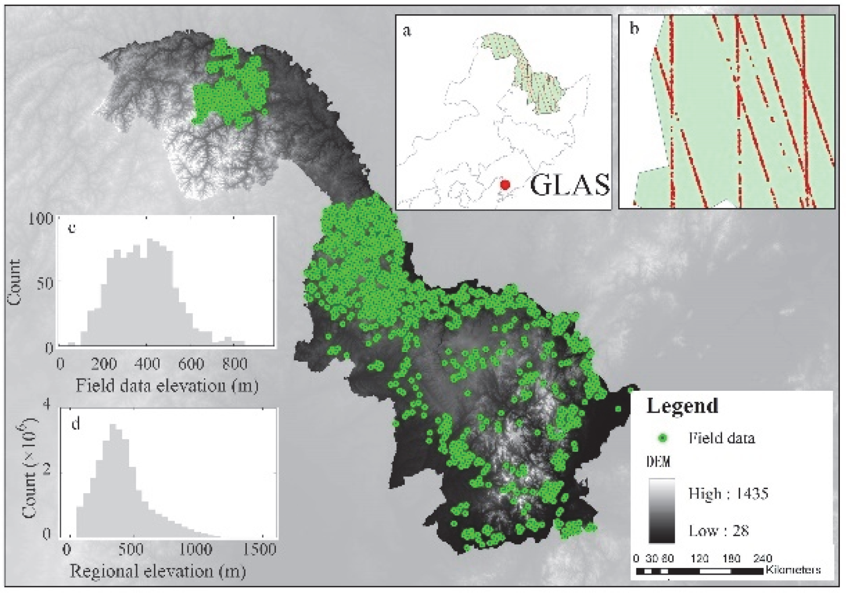
2.1. Study Area

The study area is in mountainous north-east China, in an area that includes the Greater and Lesser Khingan Mountains (Figure 1). The region provides both ecological security shelter timber and commercial timber, and makes up a large proportion of the total forest biomass of China. The Greater Khingan Mountains are located in the northernmost part of China, and have a cold temperate continental monsoon climate. The Lesser Khingan Mountains have a temperate continental monsoon climate and are located to the southeast of Greater Khingan. In our study area, the annual mean temperature ranges from −7 to 5 °C. Annual precipitation ranges from 400 to 650 mm, 80% of which falls in the wet season (May to September). Forest covers 75.6% of the region, with the major forest types being cold-temperate conifer forests and temperate deciduous broadleaf mixed forests. The most abundant species include Betula platyphylla, Larix gmelin, Populus davidiana, Quercus mongolica, Betula davurica, Salix taraikensis, and Picea koraiensis [41]. The topography varies greatly, with 34.0% of the area having rugged terrain with slopes greater than 5°, and a mean elevation of 404 m. The area is a valuable ‘laboratory’ for mountain forest AGB estimation.

2.2. Data Collection

2.2.1. Forest Inventory Data

In 2008, we created a dataset containing 1058 field measurements to use in the comparison of the performance of multi-source data and for the validation of wall-to-wall forest AGB mapping. The field measurements followed a uniform systematic inventory protocol. Each plot covers an area of 100 m × 100 m. For each plot, the tree type, tree height, and diameter at breast height (DBH) of all the trees within the plot having a DBH ≥ 5 cm were measured, and the forest AGB at plot scale was calculated following the bookkeeping model employed in previous analyses [36,42,43]. The field measurements of forest AGB range from 1.1 to 230 Mg ha−1 (1 Mg = 106 g), with a mean value of 60.35 Mg ha−1.

2.2.2. Remote Sensing Data

The Geoscience Laser Altimeter System (GLAS) instrument onboard the NASA Ice, Cloud, and land Elevation satellite (ICESat) orbited from January 2003 until 2009, and provided the forest vertical structure from systematic laser samples. The footprint of ICESat/GLAS has a diameter of ~65 m on the ground, separated by ~170 m along the track. The track-spacing varied from 5 km at high latitudes to 30 km at the Equator [32]. The GLAS system provided users with 15 science data products, named GLA01 to GLA15. In this study, we obtained GLA01 from Version 33, and GLA05 and GLA14 from Version 34. GLA01 recorded the received waveform required to extract forest height from the data with a vertical resolution of 15 cm. GLA14 provided the land-surface altimetry product with accurate footprint centroid location, and GLA05 offered the range correction data based on the original waveform. We selected data from the L3J (February–March 2008) and L3K campaigns (October 2008) to match the field data acquisition time. GLAS footprints were filtered further using the following four criteria to ensure the quality of each footprint: (1) exclude footprints taken during the presence of clouds; (2) ignore the saturated footprint if the saturation correction flag (sat_corr_flg) is greater than 2; (3) ignore noise-contaminated waveform if the signal to noise ratio is less than 50 [44]; (4) exclude footprints if the difference between GLAS elevation and SRTM elevation exceeds 7 m [26,45]. With the data filtered in this way, we obtained 1814 GLAS footprints with acceptable quality across the study region.

2.2.3. ALOS PALSAR

PALSAR is a synthetic aperture radar sensor onboard the ALOS satellite, which provides a variety of different polarization mode information, with the combination of different polarization patterns potentially enhancing the degree of feature recognition. Therefore, we extracted the L-band Digital Number ( D N ) of dual-polarization modes from the PALSAR data at 10 m resolution during the growing season of 2008. Here, dual-polarization modes include both the HH (horizontal–horizontal) and HV (horizontal–vertical) mode. Then, the DN value of the original data was converted to a backscatter coefficient (γ0) according to the PALSAR calibration factor ( C   = −83 dB):
γ 0 = 10 × l o g 10 D N 2 + C
To eliminate the speckle effect, we filtered the images at 10 m resolution with a Lee Filter using a 5 × 5 window. Considering inland water bodies may potentially affect the backscatter information, we replaced pixels located within 1 km of water bodies with the nearest grid value with the same land cover type. Finally, we calculated the difference and ratio of polarization patterns (i.e., HH-HV, HH/HV) to enhance the forest information features in the images. We also resampled the data to 100 m to match the sample data. The dataset we obtained was carefully radiometric and geometric corrected, which removed the misleading topographic influence on the backscatter coefficient, and corrected the geometric distortions caused by side-looking.

2.2.4. MODIS

We obtained optical information for the 2008 growing season from the MODIS instrument aboard the Terra satellite. The optical products consist of the Nadir BRDF-Adjusted (Bidirectional reflectance distribution function) reflectance (NBAR), Normalized Difference Vegetation Index (NDVI), Enhanced Vegetation Index (EVI), Vegetation Continuous Fields (VCF), and Leaf Area Index (LAI). MODIS-based data were resampled to 100 m. The quality flag was used to ensure high-quality estimation, and pixels in the 2008 data flagged as low quality were replaced with high-quality data obtained during the growing season in adjacent years. Previous research has demonstrated the utility of these three datasets for forest structure estimation [46,47,48].
The NBAR spectral bands (1–7) use reflectance data provided the by MCD43A2 product with a spatial resolution of 500 m × 500 m. A transformation is applied to the data to make it appear as if the data for each pixel were collected from directly overhead (i.e., the nadir point of view). The NBAR product is retrieved using a semi-empirical BRDF model with RossThick-LiSparse kernel functions [49,50,51,52]. The continuous forest cover properties were provided by the VCF data, which are compiled from a globally validated MOD44B dataset at a spatial resolution of 250 m × 250 m. Yearly VCF was produced from all seven bands of land-surface reflectance and land-surface temperature, which represent the subpixel heterogeneity, and outperform the traditional discrete classifications [53]. LAI, defined as one-half of the total leaf area per unit horizontal ground surface area, was used to describe the canopy foliage content and crown structure [54]. We derived the LAI dataset from the global land-surface satellite (GLASS) dataset with 8-day temporal resolution and 1 km × 1 km spatial resolution (http://www.glass.umd.edu/, accessed on 1 October 2021) [55].

2.2.5. Ancillary Data
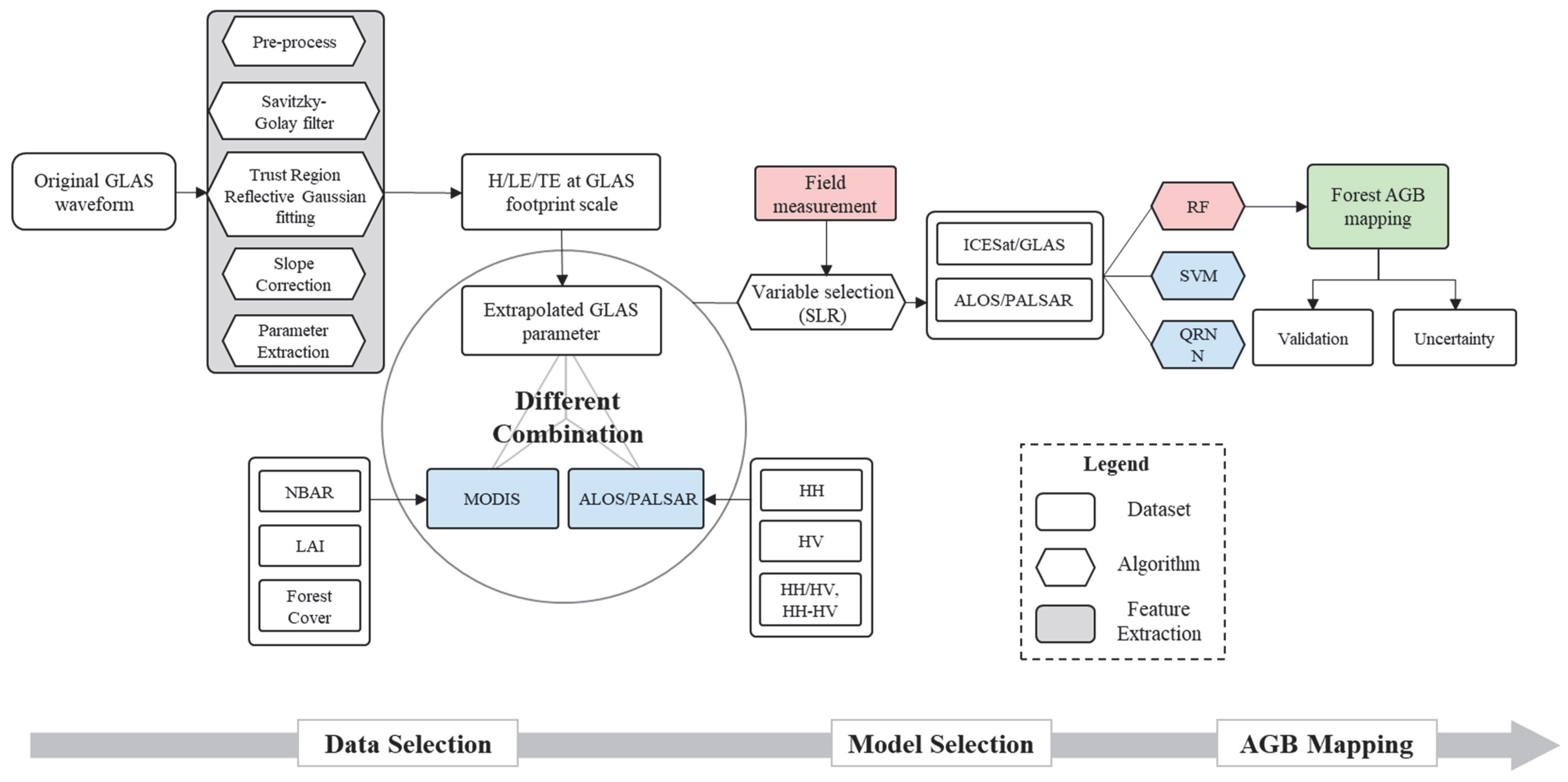
Slope data were obtained from digital elevation models with full coverage, and 3-arc seconds resolution (approximately 90 m) from the Shuttle Radar Topography Mission (SRTM), which were provided by the Consortium for Spatial Information of the Consultative Group for International Agricultural Research (CGIAR-CSI) version 4.1 dataset. The slope information for each pixel was derived by using the Arcgis 10.1 “Slope” function. Forest regions were defined by the 1:1,000,000 vegetation map of China.

3. Method

A schematic illustrating the process used in this study is shown in Figure 2. We first obtained multi-source data at the field-measured plot scale, and then diagnosed the performance of these data and different algorithms. Based on the parsimonious data source combination, we then produced the map of forest AGB and its uncertainty for the mountainous region of north-eastern China under study.

3.1. ICESat/GLAS Waveform Feature Extraction

We derived three forest structure features, vegetation canopy height (H), leading edge extent (LEE), and trailing edge extent (TEE) from the ICESat/GLAS waveform data.
To extract H, we used the mechanism-based procedure proposed by Wang et al. [40], which has been confirmed to be effective over mountainous regions [46,56]. We further extracted LEE and TEE following the method of Lefsky et al. [35] but based on the processed waveform as follows. Firstly, the original GLAS waveform was filtered using the Savitzky–Golay algorithm and then decomposed into a multiple Gaussian decomposition using the Trust Region Reflective algorithm. The decomposed waveform parameters are listed in Table 1. Then, the start and end of signal (SigBegslope and SigEndslope; also refer to Table 1) were defined with a signal cumulative distribution function. The topography-influenced waveform was corrected according to the broadened ground return caused by terrain variation. Full details of this correction are given by Wang et al. [40]. Finally, the three forest structure features, H, LEE, and TEE, were calculated based on the corrected waveform using the equations given in Table 1.
To maintain the best quality data, we further screened the GLAS-derived features following the procedure set out by Los et al. [45]. We excluded footprints with weak signal strengths, defined as the area under the first Gaussian being less than 1 V ns or the amplitude of the first Gaussian being less than 0.05 V. We also excluded footprints with slopes larger than 25°, since they were composed of a mixture of ground and canopy returns. The exclusion of these steeply sloping footprints was supported by three-dimensional simulations [40,57].
Furthermore, we extrapolated the GLAS footprint scale features to the regional scale with the inverse distance kernel kriging method used by Mitchard et al. [58] This method has an advantage over the traditional regression method since it preserves the biological meaning of plot data [59].

3.2. Biomass Modeling

We first considered a simple method, stepwise linear regression (SLR), to determine the strength of the relationship between different source data and forest AGB (Table 2). SLR builds the multiple linear regressions iteratively using a stepwise method. The only user-defined parameter is an accuracy estimation method, meaning parameter-related uncertainty is kept to a minimum. SLR has been widely used for feature selection [27,31]. Next, we compared the performance of three widely used machine-learning algorithms: Quantile Regression Neural Network (QRNN); Support Vector Machine (SVM); and Random Forest (RF). QRNN is based on an artificial neural network with the analog of linear quantile regression, which implements a differentiable approximation to the cost function to obtain a simplified form of the finite smoothing algorithm [60,61]. To obtain the nonlinear model, the hidden-layer transfer function was defined as sigmoid. SVM determines a hyperactive plane to minimize the structural risk [62]. Here, we adopted the C-SVM classifier with a radial basis function (RBF) kernel provided in R. RF is a combination of unpruned regression trees, which are generated from bootstrap samples of the various features [63]. The prediction is optimized by aggregating the ensembles. Table 3 shows the detailed parameter settings and the results for the different algorithms.

3.3. Uncertainty Analysis

At the plot scale, 10-fold cross-validation was used to assess the accuracy of multi-source features. In this method, the original set of field measurements is randomly shuffled into ten sets of equal size. One round of cross-validation would perform the analysis on nine subsets (training samples), and validate on the remaining subset (validation samples). The cross-validation process is then repeated ten times to reduce the variability, and so each sample is used exactly once as the validation data.
Additionally, in the regional mapping step, we randomly reserved 5% of the field biomass measurements to independently estimate the uncertainty of regional forest AGB mapping at the field measurements level. Here, the coefficient of determination (R2), root mean square error (RMSE), and relative RMSE (RMSE%) were used to quantify the algorithm performance. To estimate uncertainties at the pixel level, we employed the bootstrapping method, in which a series of alternative datasets, with the replacement of random samples, are constructed, and the standard deviation of 1000 iterations is used to evaluate the prediction uncertainty [64].

4. Result and Discussion

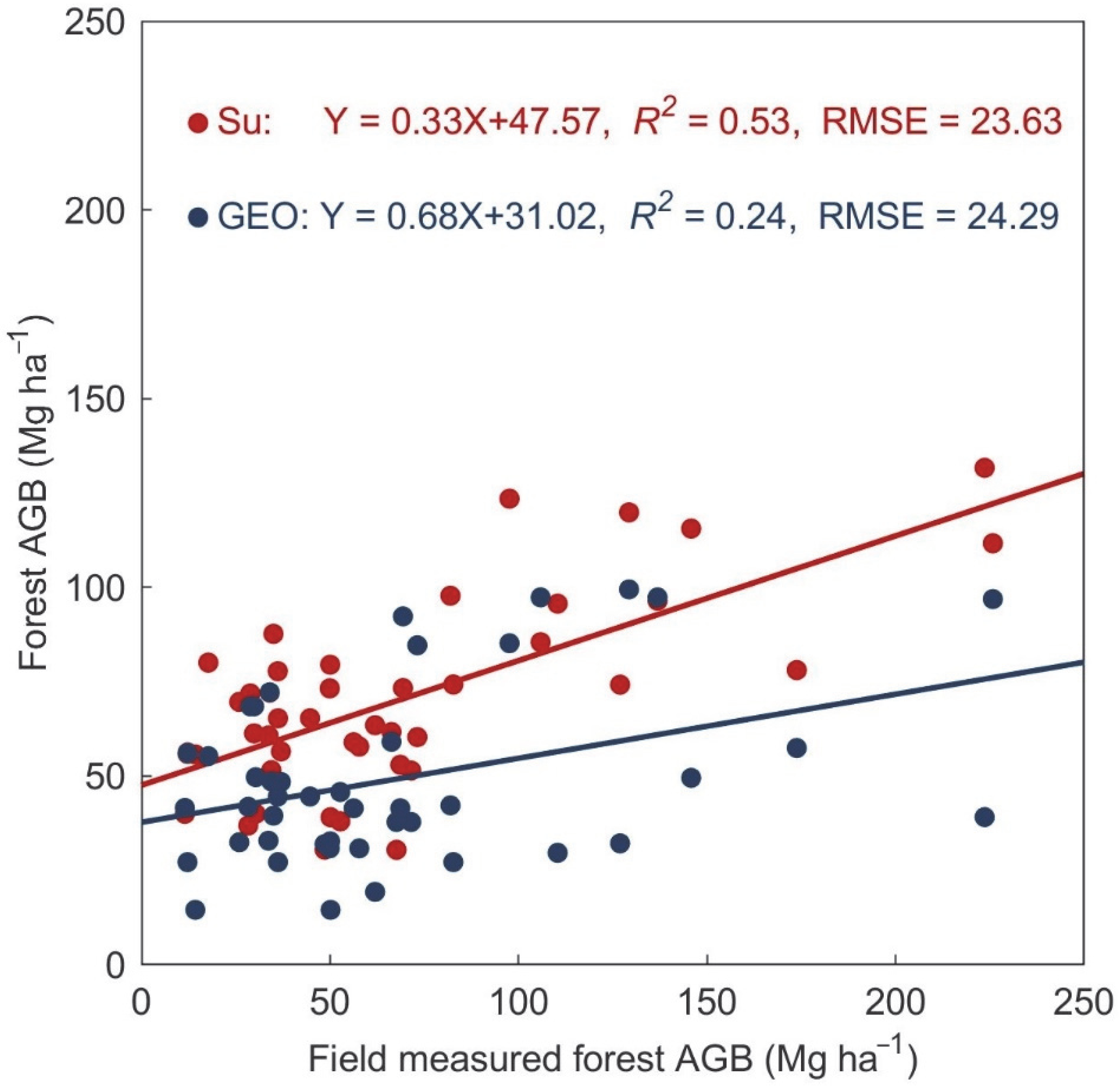
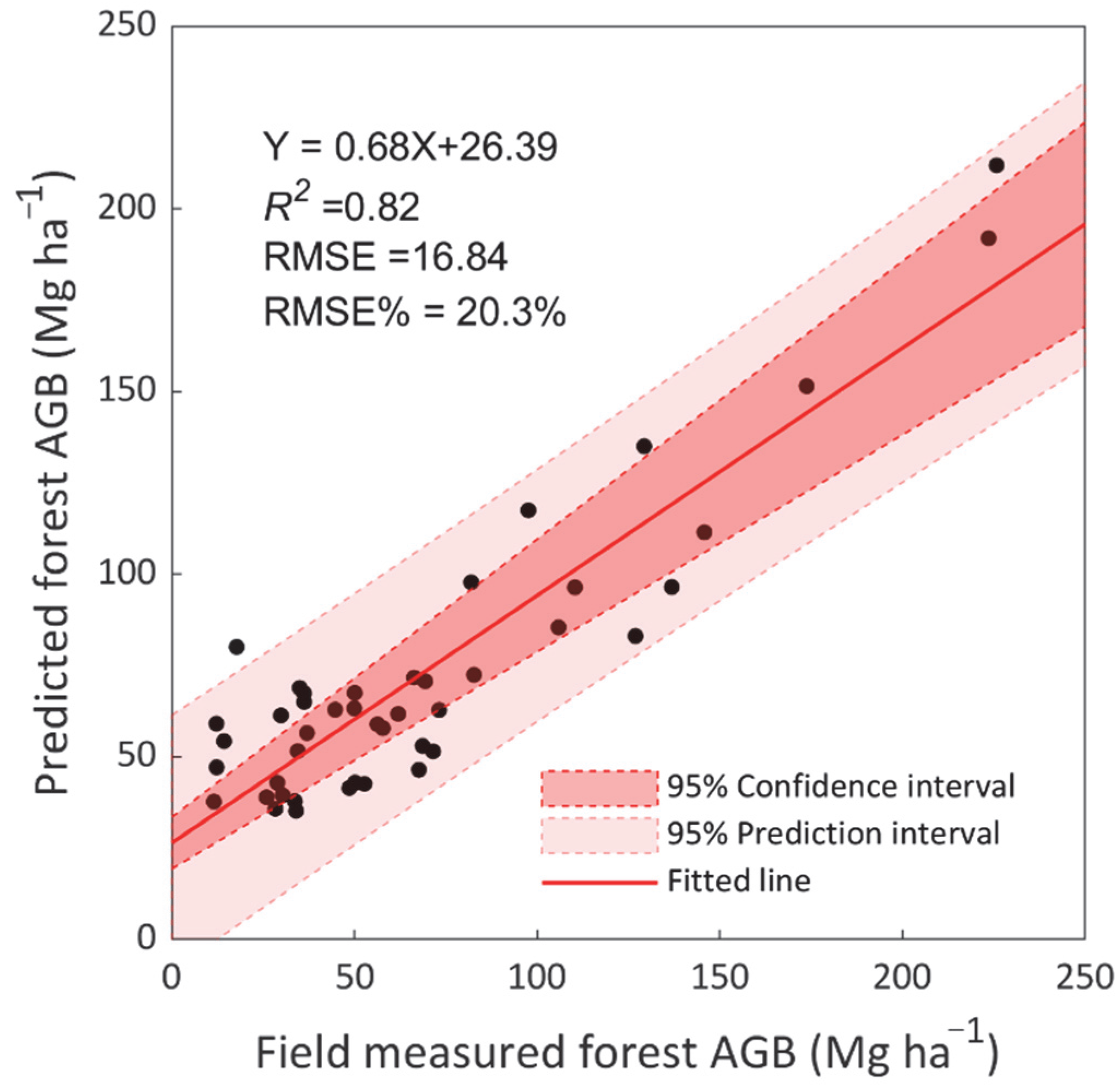
4.1. Performance of Multi-Source Remote Sensing Features for Biomass Estimation at the Plot Scale

We first analyzed biomass estimation using optical, SAR, and LiDAR separately, and then tested the combinations of those data sources, in terms of R2 and RMSE with 10-fold cross validation. Here, to eliminate the uncertainty caused by parameter setting in complex machine-learning methods, the simple stepwise linear regression algorithm was adopted to evaluate the strength of the relationship between different features and forest AGB. The results are shown in Table 2. GLAS-based estimation outperformed estimation based on both MODIS and PALSAR data, as might be expected when single source data are considered. Forest reflectance derived from MODIS data has a relatively low correlation with AGB, and the goodness of fit (R2) is only 0.15. Forest backscatter information extracted from PALSAR has better AGB estimation capability than that from MODIS, with an improved R2 value of 0.25, while the RMSE only decreased by 3.1%. Forest vertical structure (H, LEE, and TEE) derived from the GLAS data reveals a good relationship with field measurements with an R2 value of 0.33. The use of improved forest canopy height raised the estimation of R2 to 0.44. The increase in R2, in this case, is probably because 31.3% of the selected plot measurements were located in mountainous regions with slopes exceeding 5°, where the algorithm proposed by Wang et al. [40] with the correction for the effect of the terrain can provide a better depiction of the forest structure.
The inclusion of an additional source of features based on GLAS data increased the accuracy of biomass prediction as illustrated by the increased R2 and decreased RMSE values. The combination of GLAS and PALSAR-derived features shows a higher correlation with the field measurements (R2 = 0.57, RMSE = 32.15 Mg ha−1) than that of the combination of GLAS and MODIS (R2 = 0.47, RMSE = 43.79 Mg ha−1). What stands out in the table is that the regression based on all three types of features (GLAS and PALSAR and MODIS) barely improved the R2 value, by 0.01, and decreased the RMSE by only 1.82 Mg ha−1, implying that the inclusion of MODIS-based features did not add much explanatory power for prediction. In addition, we also tested the alpha significance ( α ) for each MODIS-based feature. The analysis shows that when we set the initial model as a combination of GLAS and PALSAR, the α for NDVI, EVI, VCF, and LAI equals 0.02, 0.11, −0.02 and −0.01, respectively, with the α for seven NBAR bands significantly lower than the abovementioned vegetation indices, which all have values lower than −0.01. Considering all the MODIS-based features have alpha significance ( α ) lower than a standard value of 0.15, they should be excluded in the further analysis.
Although previous analyses have indicated that the use of LiDAR-based features is promising for estimating forest AGB, barely any quantitative analyses reveal the contribution of forest vertical structure measurements to accurate AGB estimation in mountainous regions. Our plot-scale comparison proved that improved forest structure features that take into account the influence of the terrain on forest vertical distribution can better characterize forest AGB by increasing R2 by 0.11, and reducing RMSE by 5.01 Mg ha−1. The result gives further weight to the idea that accurate estimation of forest canopy height, especially in mountainous regions, is a necessary basis for accurate AGB estimation [46]. Compared with the GLAS and PALSAR combination, the improvement in the prediction results from the combination of three datasets (when additional variables from MODIS are included) is negligible. This result challenges the notion that more prediction variables would always benefit the regression, and could stem from the fact that there are hidden relationships between the different datasets. PALSAR-based features contain horizontal property information for forest regions [65,66], which might correlate with MODIS-based horizontal forest property features [67]. The additional information from the MODIS data would, in that case, introduce redundancy and increase the risk of overfitting. In addition, PALSAR- and GLAS-based features contain a vertical structure distribution, which provides important measures to characterize biomass. Considering the trade-off between accuracy and efficiency, we used the parsimonious combination of GLAS- and PALSAR-based features to produce the regional forest AGB map. Therefore, based on our comparison of multi-source remote sensing data, we emphasize the importance of data selection before biomass modeling.

4.2. Performance of Different Algorithms for Biomass Estimation at the Plot Scale

This section of the comparison is concerned with the performance of the different algorithms. RF produced the best results, followed by SVM, QRNN, and SLR. SLR is one of the most intuitive algorithms, with no parameter setting needed, and is suitable for feature selection, although the assumption of a linear correlation between different features and AGB may limit its performance. The flexible structure of QRNN and its capacity for identifying complex nonlinear relationships make it a better choice for our research. Since the prediction capability of SVM strongly depends on the selection of values for the parameters cost and gamma, we used a cross-validation method to select an optimal parameter combination. We defined a relatively large value for the gamma of 32 to ensure that enough support vectors are included to divide the feature space. During the RF model training, we identified the optimum parameter by comparing results with the number of trees (T) ranging from 100 to 1000, with an interval of 100 (Table 3). The model error declined rapidly when T increased from 100 to 500, but with little or no reduction in error with more than 500 trees, and in this way, we adopted a relatively large number of trees (T = 500) to confirm the stability of the regression result. In addition, the number of variables at each node was set as the square root of the number of features [68]. Table 3 shows that RF achieved the best prediction result, explaining 81% of the forest AGB. It is followed closely by SVM, which explains 79%. Both RF and SVM reveal good intrinsic generalization ability with acceptable RMSE values of 18.43 and 21.53 Mg ha−1, respectively. The good prediction ability of SVM may be due to its conceptual design, which has no prior assumption such as normality or independence, and can deal with spatial heterogeneity and unevenly distributed training samples [69,70]. We ascribe the best performance of RF to its flexibility, which aggregates a set of low-bias, high-variance decision trees. As a result, it can better exploit the predictive power of all the variables and obtain the best prediction. Regarding the generality of our model selection, a series of studies have reported the superiority of RF over other algorithms using different datasets [71,72,73], which shows the algorithm selection is relatively independent of the data property. Although we should note that our selection is mainly based on R2 and RMSE, other criteria should be included to satisfy specific criteria, e.g., Powell [74] indicated that RF is less effective for maintaining the variance of observation.

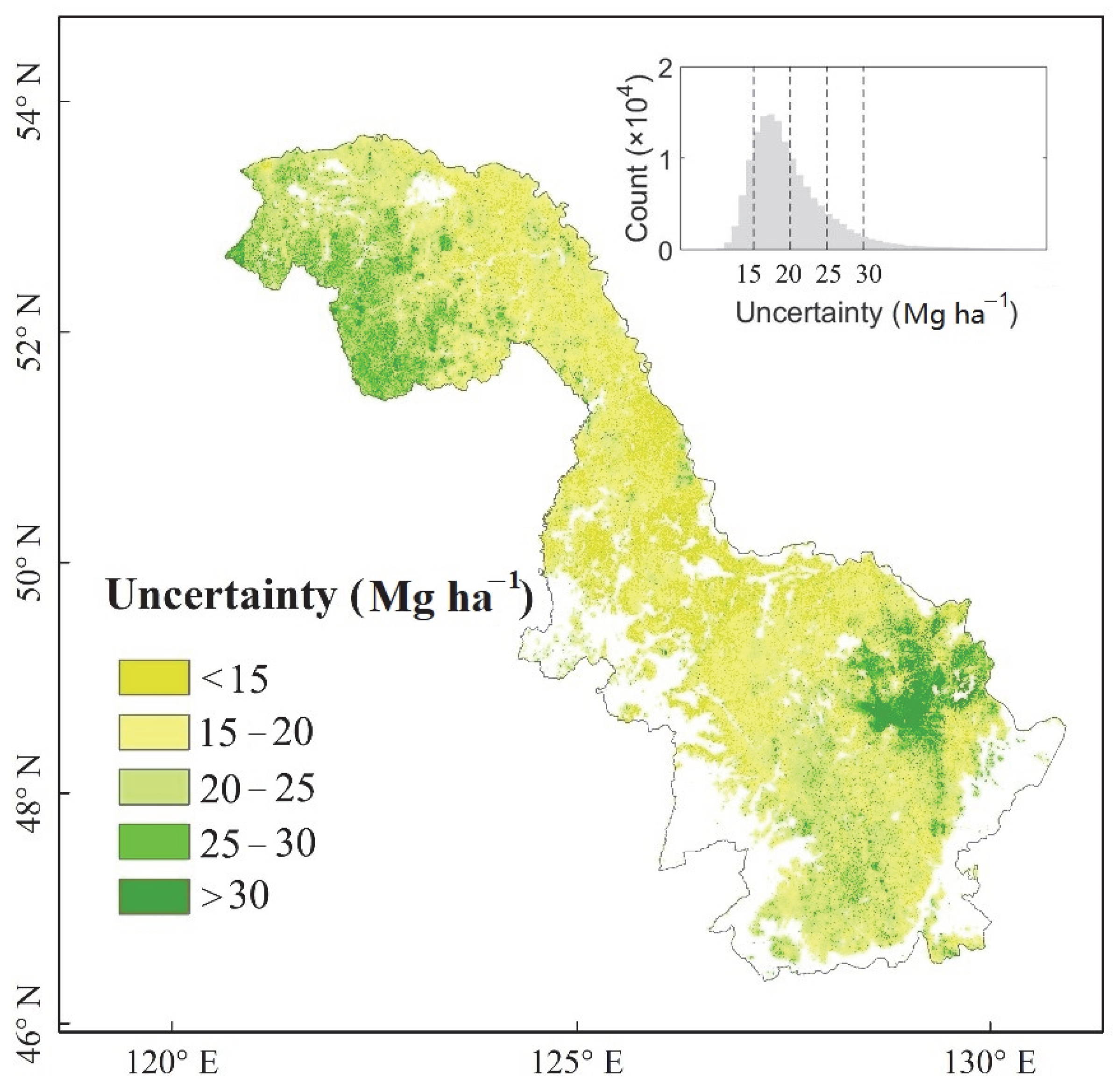
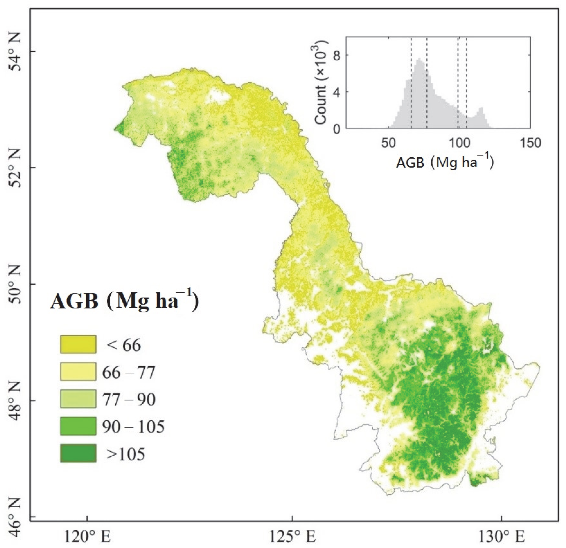
4.3. Forest Biomass Mapping for the Khingan Mountains of North-Eastern China

Based on the results of the plot-scale analysis, we combined two sources of remote sensing information: ICESat/GLAS-based forest vertical structure features and the ALOS/PALSAR backscatter coefficient data. Figure 3 is an independent validation scatterplot of a randomly selected 5% of the field measurements of AGB against the values calculated using this parsimonious data source combination and RF algorithm. The method used in our study can effectively estimate the forest AGB for both training datasets (R2 = 0.81, RMSE = 18.43 Mg ha−1, shown in Table 3) and independent validation datasets (R2 = 0.82, RMSE = 16.84 Mg ha−1, shown in Figure 3). It should be noted that the method does slightly underestimate forest AGB for observed values exceeding 150 Mg ha−1.
Since the field measurement validation reveals satisfactory results, we then produced the map of forest AGB calibrated by field measurements (Figure 4). Based on our wall-to-wall forest AGB mapping, the Khingan Mountains of north-eastern China has a range of 79.81 ± 16.00 Mg ha−1. For most (53.63%) of the region, AGB values are between 60 and 80 Mg ha−1, whereas only 13.64% of the region has forest AGB values greater than 100 Mg ha−1. The histogram of forest AGB, depicted in Figure 4, has a bimodal distribution with peaks at 70.32 and 114.72 Mg ha−1, respectively. The bimodal form of the distribution is probably due to the strong spatial gradient from south to north. The northern part of the region (Greater Khingan) has forest AGB in the range of 71.11 ± 10.9 Mg ha−1. Both low annual mean temperature (−4.2 °C) and low median annual rainfall (463.18 mm) contribute to the relatively low forest AGB in this area. The southern part of the region (Lesser Khingan) has relatively large forest AGB with a mean value of 82.8 Mg ha−1 and a standard deviation of 17.6 Mg ha−1. The annual mean temperature in this southern part of the region is 0.43 °C, and there is relatively high annual rainfall with large spatial variation (545.71 ± 43.45 mm). Aspect has little effect on the regional AGB distribution, with sunny (73.3 ± 15.5 Mg ha−1) and shady slopes (79.9 ± 16.0 Mg ha−1) having similar values.
We quantified the uncertainty of the predicted forest AGB values. The results are shown in the map in Figure 5. For most of the region, the uncertainty is low, at less than 25 Mg ha−1, giving confidence in the estimates for mountainous forest AGB. There is, however, a relatively large uncertainty (>30 Mg ha−1) in the eastern part of the Lesser Khingan Mountains, and we attribute this to two potential sources. Firstly, RF could not achieve a consistent modeling result in this region due to the heterogeneity of forest AGB and, secondly, there were not enough GLAS footprint data to capture the forest AGB pattern in the complex terrain of this region. Based on our estimation of AGB, and assuming that forest aboveground biomass was converted to carbon with a coefficient of 0.5 [75], the aboveground carbon stock aggregated to the regional scale is approximately 0.63 ± 0.15 Pg C (1 Pg = 1015 g).
We compared our results with two existing datasets published by Su et al. [44] and GEOCARBON [76,77] (Figure 6), hereafter referred to as the ‘Su’ and ‘Geo’ maps respectively. Su maps adopted the RF algorithm, which combines MODIS, ICESat/GLAS-based forest structure parameters, a digital elevation model from SRTM, and climate variables. We validated the map with the same set of randomly selected field data used for the scatter analysis presented in Figure 2. The Su map has a relatively strong relationship to the validation data, with an R2 value of 0.53 and RMSE of 23.63 Mg ha−1, and it significantly underestimated forest AGB for values exceeding 100 Mg ha−1. The regional mean forest AGB for our study region is estimated to be 73.5 Mg ha−1, which is 6.31 Mg ha−1 less than our assessment. This disagreement would lead to a relatively large underestimation of carbon stocks of 0.05 Pg C (~8%). The underestimation is the integrated result of the overestimation of GLAS-based features, and also the underestimation of reflectance in the optical images at high AGB levels. The influence of the terrain on waveform features was not taken into account in the creation of the Su map, so the canopy height, LEE, and TEE would tend to be overestimated, leading to the overestimation of forest AGB. The low penetration of optical images would also tend to cause the underestimation of forest AGB. Another important source of undervaluation may be that the few field measurements available for the Khingan Mountain region are not fully representative of the regional AGB. The GEOCARBON map is less correlated with field measurements (R2 = 0.24, RMSE 24.29 Mg ha−1), and gives a significantly lower value of 59.8 ± 20.9 Mg ha−1 for the regional forest AGB, underestimating the carbon stocks by 0.47 Pg C (~25%) compared to our study. In this case, the underestimation is probably due to the saturation of the C band Envisat ASAR at relatively high levels of forest AGB. We attribute our more accurate estimation to the improved capability of SAR data and the use of the GLAS-derived distribution of vertical forest features, which was not previously feasible. The results show that carbon storage in this region is slightly greater than previous remote sensing-based estimates. The role of mountain forests in the global carbon cycle needs further examination.

4.4. Limitation

Any bias in forest AGB estimates potentially stems from four sources: (1) The degree to which the field measurements represent both the spatial and statistical distributions of the data. (2) The pre-processing and selection of images could potentially have an influence on the results. Uncertainties may be partly derived from layover, shadowing effects, uncorrected local incident angle [78], and uncorrected topographic effects due to the coarse resolution of SRTM information. In addition, we used the growing season images, and the difference in vegetation vitality may have a seasonal effect for deciduous trees. (3) The uncertainties inherent in interpolating and extrapolating forest vertical structures with the kriging method. Although kriging preserves the biophysical meaning of forest structures, spatial heterogeneity and the uneven distribution of the GLAS footprints would introduce uncertainty in their estimation. The wall-to-wall mapping of GLAS-based features deserves more dedicated development. (4) The uncertainty of forest AGB prediction. In the present study, we only considered remotely sensed data, but the climate and local conditions, which determine the distribution of forest and shape the characteristics of the forest, should be included in future studies to estimate regional forest AGB. To undertake a comprehensive analysis of the uncertainties in forest AGB estimation, a single error propagation formula [79], which incorporates the errors from measurement at tree level, forest AGB estimation using allometric models, and sampling distribution, should be used. In addition, considering the complexity of forest AGB distribution and availability of field measurements, whether the parsimonious data source combination constructed in our study is applicable to other regions, especially in tropical areas [10], still needs further exploration.

5. Conclusions

This study makes several important contributions to furthering the understanding of regional carbon dynamics. Firstly, it provides a comprehensive method to produce spatially explicit estimates of forest AGB that is suitable for mountainous regions. Combined with GEDI data, it has the potential to be used or adapted for creating regional carbon budget estimates. The efficacy of the method is due to the inclusion of the improved GLAS-based algorithm and the use of a systematic comparison involving different remote sensing data sources and several different machine-learning algorithms. Secondly, the results provide a benchmark for regional carbon storage at 100 m resolution in 2008, which will help to improve understanding of the capacity of forests to alleviate the effects of global climatic change in future climate scenarios. It also provides a valuable dataset for Earth System Model parameterization, and may be useful for improving the simulation of the productivity of forests in mountainous regions. Thirdly, our work shows that previous studies underestimated the aboveground forest carbon stock in our study region, probably due to the saturation of remote-sensing signals at high biomass values or the complicating effects of rugged terrain on LiDAR-based measurements. We have shown that future studies on carbon stocks in mountainous forest regions should focus on the use of terrain-corrected remote sensing data and advanced machine algorithms, to gain a better picture of the forest carbon storage and its contribution to global carbon dynamics.

Author Contributions

Conceptualization, X.W., C.L. and G.C.; methodology, X.W., G.L., J.X. All authors contributed to the interpretation of the results and to the text. All authors have read and agreed to the published version of the manuscript.

Funding

This study was funded by the National Natural Science Foundation of China (41801097, 4197071437) and the Key Research and Development Programs for Global Change and Adaptation (2017YFA0603604).

Institutional Review Board Statement

Not applicable.

Informed Consent Statement

Not applicable.

Data Availability Statement

All data needed to evaluate the conclusions in this paper are present in the paper.

Acknowledgments

The authors would like to thank the National Snow and Ice Data Center for the free use of Geoscience Laser Altimeter System (GLAS) data, the Consortium for Spatial Information for distributing Shuttle Radar Topography Mission (SRTM) data.

Conflicts of Interest

The authors declare no conflict of interest.

References

  1. Beer, C.; Reichstein, M.; Tomelleri, E.; Ciais, P.; Jung, M.; Carvalhais, N.; Rödenbeck, C.; Arain, M.A.; Baldocchi, D.; Bonan, G.B. Terrestrial gross carbon dioxide uptake: Global distribution and covariation with climate. Science 2010, 329, 834–838. [Google Scholar] [CrossRef] [PubMed] [Green Version]
  2. Bonan, G. Carbon cycle: Fertilizing change. Nat. Geosci. 2008, 1, 645. [Google Scholar] [CrossRef]
  3. Pan, Y.; Birdsey, R.A.; Fang, J.; Houghton, R.; Kauppi, P.E.; Kurz, W.A.; Phillips, O.L.; Shvidenko, A.; Lewis, S.L.; Canadell, J.G. A large and persistent carbon sink in the world’s forests. Science 2011, 333, 1201609. [Google Scholar] [CrossRef] [Green Version]
  4. Houghton, R. Aboveground forest biomass and the global carbon balance. Glob. Chang. Biol. 2005, 11, 945–958. [Google Scholar] [CrossRef]
  5. Fang, J.; Chen, A.; Peng, C.; Zhao, S.; Ci, L. Changes in forest biomass carbon storage in China between 1949 and 1998. Science 2001, 292, 2320–2322. [Google Scholar] [CrossRef] [PubMed]
  6. Hawbaker, T.J.; Keuler, N.S.; Lesak, A.A.; Gobakken, T.; Contrucci, K.; Radeloff, V.C. Improved estimates of forest vegetation structure and biomass with a LiDAR-optimized sampling design. J. Geophys. Res. Biogeosci. 2009, 114. [Google Scholar] [CrossRef]
  7. Zhao, P.; Lu, D.; Wang, G.; Wu, C.; Huang, Y.; Yu, S. Examining spectral reflectance saturation in Landsat imagery and corresponding solutions to improve forest aboveground biomass estimation. Remote Sens. 2016, 8, 469. [Google Scholar] [CrossRef] [Green Version]
  8. Antropov, O.; Rauste, Y.; Häme, T.; Praks, J. Polarimetric ALOS PALSAR Time Series in Mapping Biomass of Boreal Forests. Remote Sens. 2017, 9, 999. [Google Scholar] [CrossRef] [Green Version]
  9. Santoro, M.; Cartus, O.; Fransson, J.E. Integration of allometric equations in the water cloud model towards an improved retrieval of forest stem volume with L-band SAR data in Sweden. Remote Sens. Environ. 2021, 253, 112235. [Google Scholar] [CrossRef]
  10. Vafaei, S.; Soosani, J.; Adeli, K.; Fadaei, H.; Naghavi, H.; Pham, T.D.; Tien Bui, D. Improving accuracy estimation of Forest Aboveground Biomass based on incorporation of ALOS-2 PALSAR-2 and Sentinel-2A imagery and machine learning: A case study of the Hyrcanian forest area (Iran). Remote Sens. 2018, 10, 172. [Google Scholar] [CrossRef] [Green Version]
  11. Santi, E.; Paloscia, S.; Pettinato, S.; Fontanelli, G.; Mura, M.; Zolli, C.; Maselli, F.; Chiesi, M.; Bottai, L.; Chirici, G. The potential of multifrequency SAR images for estimating forest biomass in Mediterranean areas. Remote Sens. Environ. 2017, 200, 63–73. [Google Scholar] [CrossRef]
  12. Zhang, L.; Shao, Z.; Liu, J.; Cheng, Q. Deep learning based retrieval of forest aboveground biomass from combined LiDAR and landsat 8 data. Remote Sens. 2019, 11, 1459. [Google Scholar] [CrossRef] [Green Version]
  13. Baghdadi, N.; El Hajj, M.; Dubois-Fernandez, P.; Zribi, M.; Belaud, G.; Cheviron, B. Signal level comparison between TerraSAR-X and COSMO-SkyMed SAR sensors. IEEE Geosci. Remote Sens. Lett. 2015, 12, 448–452. [Google Scholar] [CrossRef] [Green Version]
  14. Ferrazzoli, P.; Guerriero, L. Radar sensitivity to tree geometry and woody volume: A model analysis. IEEE Trans. Geosci. Remote Sens. 1995, 33, 360–371. [Google Scholar] [CrossRef]
  15. Joshi, N.P.; Mitchard, E.T.; Schumacher, J.; Johannsen, V.K.; Saatchi, S.; Fensholt, R. L-band SAR backscatter related to forest cover, height and aboveground biomass at multiple spatial scales across Denmark. Remote Sens. 2015, 7, 4442–4472. [Google Scholar] [CrossRef] [Green Version]
  16. Luckman, A.; Baker, J.; Kuplich, T.M.; Yanasse, C.d.C.F.; Frery, A.C. A study of the relationship between radar backscatter and regenerating tropical forest biomass for spaceborne SAR instruments. Remote Sens. Environ. 1997, 60, 1–13. [Google Scholar] [CrossRef]
  17. Baghdadi, N.; Le Maire, G.; Bailly, J.-S.; Osé, K.; Nouvellon, Y.; Zribi, M.; Lemos, C.; Hakamada, R. Evaluation of ALOS/PALSAR L-band data for the estimation of Eucalyptus plantations aboveground biomass in Brazil. IEEE J. Sel. Top. Appl. Earth Obs. Remote Sens. 2015, 8, 3802–3811. [Google Scholar] [CrossRef] [Green Version]
  18. Mitchard, E.T.; Saatchi, S.S.; Woodhouse, I.H.; Nangendo, G.; Ribeiro, N.; Williams, M.; Ryan, C.M.; Lewis, S.L.; Feldpausch, T.; Meir, P. Using satellite radar backscatter to predict above-ground woody biomass: A consistent relationship across four different African landscapes. Geophys. Res. Lett. 2009, 36, 1–7. [Google Scholar] [CrossRef]
  19. Santos, J.; Lacruz, M.P.; Araujo, L.; Keil, M. Savanna and tropical rainforest biomass estimation and spatialization using JERS-1 data. Int. J. Remote Sens. 2002, 23, 1217–1229. [Google Scholar] [CrossRef]
  20. Neeff, T.; Dutra, L.V.; dos Santos, J.R.; Freitas, C.d.C.; Araujo, L.S. Tropical forest measurement by interferometric height modeling and P-band radar backscatter. For. Sci. 2005, 51, 585–594. [Google Scholar]
  21. Lefsky, M.A.; Harding, D.J.; Keller, M.; Cohen, W.B.; Carabajal, C.C.; Del Bom Espirito-Santo, F.; Hunter, M.O.; de Oliveira, R. Estimates of forest canopy height and aboveground biomass using ICESat. Geophys. Res. Lett. 2005, 32, 1–4. [Google Scholar] [CrossRef] [Green Version]
  22. Pang, Y.; Lefsky, M.; Andersen, H.-E.; Miller, M.E.; Sherrill, K. Validation of the ICEsat vegetation product using crown-area-weighted mean height derived using crown delineation with discrete return lidar data. Can. J. Remote Sens. 2008, 34, S471–S484. [Google Scholar] [CrossRef]
  23. Walter, J.D.; Edwards, J.; McDonald, G.; Kuchel, H. Estimating biomass and canopy height with LiDAR for field crop breeding. Front. Plant Sci. 2019, 10, 1145. [Google Scholar] [CrossRef] [PubMed]
  24. Mitchard, E.T.; Saatchi, S.S.; White, L.; Abernethy, K.; Jeffery, K.J.; Lewis, S.L.; Collins, M.; Lefsky, M.A.; Leal, M.E.; Woodhouse, I.H. Mapping tropical forest biomass with radar and spaceborne LiDAR in Lopé National Park, Gabon: Overcoming problems of high biomass and persistent cloud. Biogeosciences 2012, 9, 179–191. [Google Scholar] [CrossRef] [Green Version]
  25. Montaghi, A.; Corona, P.; Dalponte, M.; Gianelle, D.; Chirici, G.; Olsson, H. Airborne laser scanning of forest resources: An overview of research in Italy as a commentary case study. Int. J. Appl. Earth Obs. Geoinf. 2013, 23, 288–300. [Google Scholar] [CrossRef] [Green Version]
  26. Baccini, A.; Goetz, S.; Walker, W.; Laporte, N.; Sun, M.; Sulla-Menashe, D.; Hackler, J.; Beck, P.; Dubayah, R.; Friedl, M. Estimated carbon dioxide emissions from tropical deforestation improved by carbon-density maps. Nat. Clim. Chang. 2012, 2, 182–185. [Google Scholar] [CrossRef]
  27. Zhang, Y.; Liang, S.; Sun, G. Forest biomass mapping of northeastern China using GLAS and MODIS data. IEEE J. Sel. Top. Appl. Earth Obs. Remote Sens. 2014, 7, 140–152. [Google Scholar] [CrossRef]
  28. Hyde, P.; Dubayah, R.; Walker, W.; Blair, J.B.; Hofton, M.; Hunsaker, C. Mappingforest structure for wildlife habitat analysis using multi-sensor (LiDAR, SAR/InSAR, ETM+, Quickbird) synergy. Remote Sens. Environ. 2006, 102, 63–73. [Google Scholar] [CrossRef]
  29. Ni, W.; Zhang, Z.; Sun, G. Assessment of Slope-Adaptive Metrics of GEDI Waveforms for Estimations of Forest Aboveground Biomass over Mountainous Areas. J. Remote Sens. 2021, 2021, 805364. [Google Scholar] [CrossRef]
  30. Wang, Y.; Ni, W.; Sun, G.; Chi, H.; Zhang, Z.; Guo, Z. Slope-adaptive waveform metrics of large footprint lidar for estimation of forest aboveground biomass. Remote Sens. Environ. 2019, 224, 386–400. [Google Scholar] [CrossRef]
  31. Chi, H.; Sun, G.; Huang, J.; Guo, Z.; Ni, W.; Fu, A. National forest aboveground biomass mapping from ICESat/GLAS data and MODIS imagery in China. Remote Sens. 2015, 7, 5534–5564. [Google Scholar] [CrossRef] [Green Version]
  32. Brenner, A.C.; Zwally, H.J.; Bentley, C.R.; Csathó, B.M.; Harding, D.J.; Minster, L.J.; Roberts, J.L.; Saba, R.H.; Thomas, D. Derivation of Range and Range Distributions from Laser Pulse Waveform Analysis for Surface Elevations, Roughness, Slope, and Vegetation Heights. Algorithm Theoretical Basis Document V4. 1. Available online: http://www.csr.utexas.edu/glas/pdf/Atbd_20031224.Pdf (accessed on 1 October 2021).
  33. Klein, T.; Randin, C.; Körner, C. Water availability predicts forest canopy height at the global scale. Ecol. Lett. 2015, 18, 1311–1320. [Google Scholar] [CrossRef] [PubMed]
  34. Körner, C. Mountain systems. In Ecosystems and Human Well-Being: Current State and Trends; Island Press: Washington, DC, USA, 2005; pp. 681–716. [Google Scholar]
  35. Lefsky, M.A.; Keller, M.; Pang, Y.; de Camargo, P.B.; Hunter, M.O. Revised method for forest canopy height estimation from Geoscience Laser Altimeter System waveforms. J. Appl. Remote Sens. 2007, 1, 013537. [Google Scholar]
  36. Chi, H.; Sun, G.; Huang, J.; Li, R.; Ren, X.; Ni, W.; Fu, A. Estimation of Forest Aboveground Biomass in Changbai Mountain Region Using ICESat/GLAS and Landsat/TM Data. Remote Sens. 2017, 9, 707. [Google Scholar] [CrossRef] [Green Version]
  37. Hilbert, C.; Schmullius, C. Influence of surface topography on ICESat/GLAS forest height estimation and waveform shape. Remote Sens. 2012, 4, 2210–2235. [Google Scholar] [CrossRef] [Green Version]
  38. Chen, Q. Retrieving vegetation height of forests and woodlands over mountainous areas in the Pacific Coast region using satellite laser altimetry. Remote Sens. Environ. 2010, 114, 1610–1627. [Google Scholar] [CrossRef]
  39. Wang, X.; Cheng, X.; Gong, P.; Huang, H.; Li, Z.; Li, X. Earth science applications of ICESat/GLAS. Int. J. Remote Sens. 2011, 32, 8837–8864. [Google Scholar] [CrossRef]
  40. Wang, X.; Huang, H.; Gong, P.; Liu, C.; Li, C.; Li, W. Forest canopy height extraction in rugged areas with ICESAT/GLAS data. IEEE Trans. Geosci. Remote Sens. 2014, 52, 4650–4657. [Google Scholar] [CrossRef]
  41. Tan, L.; Zhang, P.; Zhao, X.; Fan, C.; Zhang, C.; Yan, Y.; Von Gadow, K. Analysing species abundance distribution patterns across sampling scales in three natural forests in Northeastern China. iForest-Biogeosci. For. 2020, 13, 482. [Google Scholar] [CrossRef]
  42. Wang, Y.; Li, G.; Ding, J.; Guo, Z.; Tang, S.; Wang, C.; Huang, Q.; Liu, R.; Chen, J.M. A combined GLAS and MODIS estimation of the global distribution of mean forest canopy height. Remote Sens. Environ. 2016, 174, 24–43. [Google Scholar] [CrossRef]
  43. Feng, Z.W.; Wang, X.K.; Wu, G. The Biomass and Productivity of China Forest Ecosystem; Science Press: Beijing, China, 1999; pp. 1–50. (In Chinese) [Google Scholar]
  44. Su, Y.; Guo, Q.; Xue, B.; Hu, T.; Alvarez, O.; Tao, S.; Fang, J. Spatial distribution of forest aboveground biomass in China: Estimation through combination of spaceborne lidar, optical imagery, and forest inventory data. Remote Sens. Environ. 2016, 173, 187–199. [Google Scholar] [CrossRef] [Green Version]
  45. Los, S.; Rosette, J.; Kljun, N.; North, P.; Chasmer, L.; Suárez, J.; Hopkinson, C.; Hill, R.; Van Gorsel, E.; Mahoney, C. Vegetation height products between 60° S and 60° N from ICESat GLAS data. Geosci. Model Dev. 2012, 5, 413–432. [Google Scholar] [CrossRef] [Green Version]
  46. Huang, H.; Liu, C.; Wang, X.; Biging, G.S.; Chen, Y.; Yang, J.; Gong, P. Mapping vegetation heights in China using slope correction ICESat data, SRTM, MODIS-derived and climate data. ISPRS J. Photogramm. Remote Sens. 2017, 129, 189–199. [Google Scholar] [CrossRef]
  47. Sun, X.; Wang, G.; Huang, M.; Chang, R.; Ran, F. Forest biomass carbon stocks and variation in Tibet’s carbon-dense forests from 2001 to 2050. Sci. Rep. 2016, 6, 34687. [Google Scholar] [CrossRef]
  48. Yin, G.; Zhang, Y.; Sun, Y.; Wang, T.; Zeng, Z.; Piao, S. MODIS based estimation of forest aboveground biomass in China. PLoS ONE 2015, 10, e0130143. [Google Scholar] [CrossRef] [Green Version]
  49. Lucht, W.; Schaaf, C.B.; Strahler, A.H. An algorithm for the retrieval of albedo from space using semiempirical BRDF models. IEEE Trans. Geosci. Remote Sens. 2000, 38, 977–998. [Google Scholar] [CrossRef] [Green Version]
  50. Schaaf, C.B.; Gao, F.; Strahler, A.H.; Lucht, W.; Li, X.; Tsang, T.; Strugnell, N.C.; Zhang, X.; Jin, Y.; Muller, J.P. First operational BRDF, albedo nadir reflectance products from MODIS. Remote Sens. Environ. 2002, 83, 135–148. [Google Scholar] [CrossRef] [Green Version]
  51. Wanner, W.; Li, X.; Strahler, A. On the derivation of kernels for kernel-driven models of bidirectional reflectance. J. Geophys. Res. Atmos. 1995, 100, 21077–21089. [Google Scholar] [CrossRef]
  52. Wanner, W.; Strahler, A.; Hu, B.; Lewis, P.; Muller, J.P.; Li, X.; Schaaf, C.; Barnsley, M. Global retrieval of bidirectional reflectance and albedo over land from EOS MODIS and MISR data: Theory and algorithm. J. Geophys. Res. Atmos. 1997, 102, 17143–17161. [Google Scholar] [CrossRef] [Green Version]
  53. Hansen, M.C.; Potapov, P.V.; Moore, R.; Hancher, M.; Turubanova, S.; Tyukavina, A.; Thau, D.; Stehman, S.; Goetz, S.; Loveland, T. High-resolution global maps of 21st-century forest cover change. Science 2013, 342, 850–853. [Google Scholar] [CrossRef] [Green Version]
  54. Tang, H.; Brolly, M.; Zhao, F.; Strahler, A.H.; Schaaf, C.L.; Ganguly, S.; Zhang, G.; Dubayah, R. Deriving and validating Leaf Area Index (LAI) at multiple spatial scales through lidar remote sensing: A case study in Sierra National Forest, CA. Remote Sens. Environ. 2014, 143, 131–141. [Google Scholar] [CrossRef]
  55. Xiao, Z.; Liang, S.; Wang, J.; Chen, P.; Yin, X.; Zhang, L.; Song, J. Use of general regression neural networks for generating the GLASS leaf area index product from time-series MODIS surface reflectance. IEEE Trans. Geosci. Remote Sens. 2014, 52, 209–223. [Google Scholar] [CrossRef]
  56. Liu, C.; Wang, X.; Huang, H.; Gong, P.; Wu, D.; Jiang, J. The importance of data type, laser spot density and modelling method for vegetation height mapping in continental China. Int. J. Remote Sens. 2016, 37, 6127–6148. [Google Scholar] [CrossRef]
  57. Sun, G.Q.; Ranson, K.J. Modeling lidar returns from forest canopies. IEEE Trans. Geosci. Remote Sens. 2000, 38, 2617–2626. [Google Scholar]
  58. Mitchard, E.T.; Feldpausch, T.R.; Brienen, R.J.; Lopez-Gonzalez, G.; Monteagudo, A.; Baker, T.R.; Phillips, O.L. Markedly divergent estimates of Amazon forest carbon density from ground plots and satellites. Glob. Ecol. Biogeogr. 2014, 23, 935–946. [Google Scholar] [CrossRef]
  59. Malhi, Y.; Wood, D.; Baker, T.R.; Wright, J.; Phillips, O.L.; Cochrane, T.; Meir, P.; Chave, J.; Almeida, S.; Arroyo, L. The regional variation of aboveground live biomass in old-growth Amazonian forests. Glob. Chang. Biol. 2006, 12, 1107–1138. [Google Scholar] [CrossRef]
  60. Cannon, A.J. Quantile regression neural networks: Implementation in R and application to precipitation downscaling. Comput. Geosci. 2011, 37, 1277–1284. [Google Scholar] [CrossRef]
  61. Zhang, B.; Sajjad, S.; Chen, K.; Zhou, L.; Zhang, Y.; Yong, K.K.; Sun, Y. Predicting tree height-diameter relationship from relative competition levels using quantile regression models for Chinese fir (Cunninghamia lanceolata) in Fujian province, China. Forests 2020, 11, 183. [Google Scholar] [CrossRef] [Green Version]
  62. Chauhan, V.K.; Dahiya, K.; Sharma, A. Problem formulations and solvers in linear SVM: A review. Artif. Intell. Rev. 2019, 52, 803–855. [Google Scholar] [CrossRef]
  63. Breiman, L. Random forests. Mach. Learn. 2001, 45, 5–32. [Google Scholar] [CrossRef] [Green Version]
  64. Efron, B.; Tibshirani, R. Bootstrap methods for standard errors, confidence intervals, and other measures of statistical accuracy. Stat. Sci. 1986, 1, 54–75. [Google Scholar] [CrossRef]
  65. Harris, N.L.; Brown, S.; Hagen, S.C.; Saatchi, S.S.; Petrova, S.; Salas, W.; Hansen, M.C.; Potapov, P.V.; Lotsch, A. Baseline map of carbon emissions from deforestation in tropical regions. Science 2012, 336, 1573–1576. [Google Scholar] [CrossRef]
  66. Bouvet, A.; Mermoz, S.; Toan, T.L.; Villard, L.; Mathieu, R.; Naidoo, L.; Asner, G.P. An above-ground biomass map of African savannahs and woodlands at 25 m resolution derived from ALOS PALSAR. Remote Sens. Environ. 2018, 206, 156–173. [Google Scholar] [CrossRef]
  67. Ma, J.; Xiao, X.; Qin, Y.; Chen, B.; Hu, Y.; Li, X.; Zhao, B. Estimating aboveground biomass of broadleaf, needleleaf, and mixed forests in northeastern China through analysis of 25m ALOS/PALSAR mosaic data. For. Ecol. Manag. 2017, 389, 199–210. [Google Scholar] [CrossRef]
  68. Gislason, P.O.; Benediktsson, J.A.; Sveinsson, J.R. Random forest classification of multisource remote sensing and geographic data, Igarss 2004. In Proceedings of the IEEE International Geoscience and Remote Sensing Symposium, Anchorage, AK, USA, 20–24 September 2004; pp. 1049–1052. [Google Scholar]
  69. Nello, C.; John, S.-T. An Introduction to Support Vector Machines and Other Kernel Based Learning Methods; Cambridge University Press: New York, NY, USA, 2000. [Google Scholar]
  70. Ding, J.; Li, F.; Yang, G.; Chen, L.; Zhang, B.; Liu, L.; Fang, K.; Qin, S.; Chen, Y.; Peng, Y. The permafrost carbon inventory on the Tibetan Plateau: A new evaluation using deep sediment cores. Glob. Chang. Biol. 2016, 22, 2688–2701. [Google Scholar] [CrossRef]
  71. Fassnacht, F.; Hartig, F.; Latifi, H.; Berger, C.; Hernández, J.; Corvalán, P.; Koch, B. Importance of sample size, data type and prediction method for remote sensing-based estimations of aboveground forest biomass. Remote Sens. Environ. 2014, 154, 102–114. [Google Scholar] [CrossRef]
  72. Gleason, C.J.; Im, J. Forest biomass estimation from airborne LiDAR data using machine learning approaches. Remote Sens. Environ. 2012, 125, 80–91. [Google Scholar] [CrossRef]
  73. Latifi, H.; Nothdurft, A.; Koch, B. Non-parametric prediction and mapping of standing timber volume and biomass in a temperate forest: Application of multiple optical/LiDAR-derived predictors. Forestry 2010, 83, 395–407. [Google Scholar] [CrossRef] [Green Version]
  74. Powell, S.L.; Cohen, W.B.; Healey, S.P.; Kennedy, R.E.; Moisen, G.G.; Pierce, K.B.; Ohmann, J.L. Quantification of live aboveground forest biomass dynamics with Landsat time-series and field inventory data: A comparison of empirical modeling approaches. Remote Sens. Environ. 2010, 114, 1053–1068. [Google Scholar] [CrossRef]
  75. Chave, J.; Andalo, C.; Brown, S.; Cairns, M.A.; Chambers, J.Q.; Eamus, D.; Fölster, H.; Fromard, F.; Higuchi, N.; Kira, T.; et al. Tree allometry and improved estimation of carbon stocks and balance in tropical forests. Oecologia 2005, 145, 87–99. [Google Scholar] [CrossRef]
  76. Avitabile, V.; Herold, M.; Heuvelink, G.; Lewis, S.; Phillips, O.; Asner, G.; Armston, J.; Asthon, P.; Banin, L.; Bayol, N. An integrated pan-tropical biomass map using multiple reference datasets. Glob. Chang. Biol. 2016, 22, 1406–1420. [Google Scholar] [CrossRef] [Green Version]
  77. Santoro, M.; Beaudoin, A.; Beer, C.; Cartus, O.; Fransson, J.E.S.; Hall, R.J.; Pathe, C.; Schmullius, C.; Schepaschenko, D.; Shvidenko, A.; et al. Forest growing stock volume of the northern hemisphere: Spatially explicit estimates for 2010 derived from Envisat ASAR. Remote Sens. Environ. 2015, 168, 316–334. [Google Scholar] [CrossRef]
  78. Huang, W.L.; Sun, G.Q.; Ni, W.J.; Zhang, Z.Y.; Dubayah, R. Sensitivity of Multi-Source SAR Backscatter to Changes in Forest Aboveground Biomass. Remote Sens. 2015, 7, 9587–9609. [Google Scholar] [CrossRef] [Green Version]
  79. Rodríguez-Veiga, P.; Saatchi, S.; Tansey, K.; Balzter, H. Magnitude, spatial distribution and uncertainty of forest biomass stocks in Mexico. Remote Sens Environ. 2016, 183, 265–281. [Google Scholar] [CrossRef] [Green Version]
Figure 1. Location of the study area along with the topography provided by SRTM (elevation ranges from 28 to 1435 m). The green points indicate the locations of field measurements. The subplot shows the distribution of ICESat/GLAS data (a) with enlarged map (b) showing details of its distribution, and histogram of elevation values for both the field plots (c) and the whole study region (d).
Remotesensing 14 01039 g001
Figure 2. Schematic of the forest AGB mapping in this study. We first extracted the GLAS-based parameters using an improved algorithm suitable for rugged areas. Then, in the data selection procedure, we compared the performance of GLAS, MODIS and PALSAR, and the combinations (GLAS + MODIS, GLAS + PALSAR, and GLAS + MODIS + PALSAR). Thirdly, the performance of three different machine-learning algorithms was evaluated. Finally, we produced the benchmark map of forest AGB and its uncertainty.
Remotesensing 14 01039 g002
Figure 3. Comparison between predicted forest above ground biomass versus independent field-measured values. The dark red region represents the 95% confidence intervals for the regression line, and the light red area shows the prediction intervals for all individual observations. Performance of the proposed method was evaluated with R2, Root Mean Square Error (RMSE) and relative RMSE (RMSE%).
Remotesensing 14 01039 g003
Figure 4. Distribution of forest aboveground biomass in the Khingan Mountains of north-eastern China in 2008. The inserted panel shows a histogram of forest AGB, with the dashed lines corresponding to the intervals displayed on the map (i.e., 66, 77, 90, 105 Mg ha−1).
Remotesensing 14 01039 g004
Figure 5. Distribution of the uncertainty of forest aboveground biomass in the Khingan Mountains of northeastern China circa 2008. The inserted panel shows a histogram of forest AGB uncertainty, with the dashed lines corresponding to the intervals displayed on the map (i.e., 15, 20, 25, 30 Mg ha−1).
Remotesensing 14 01039 g005
Figure 6. Comparison of two existing maps versus independent field-measured values (same as Figure 3). Performance of those two maps was evaluated with R2, Root Mean Square Error (RMSE) and relative RMSE (RMSE%).
Remotesensing 14 01039 g006
Table 1. Description of the GLAS-derived waveform parameters derived following Wang et al., (2014).
ParametersDescriptionEquation
gpCntRng (i)Centroid of each Gaussian peak-
numPeakNumber of fitted Gaussian results
(no limitation for the maximum number)
Gsigma (i)Sigma of each Gaussian result
Gamp (i)Amplitude of each Gaussian result
Garea (i)Area under each Gaussian result
e_meanpower (i)Elevation of mean power above the background noise
SigBeg, SigEndBeginning and end of signal without terrain correction S i g B e g = μ 3 σ
S i g E n d = μ + 3 σ
Where   μ   and   σ are the estimated mean and standard deviation of the first Gaussian decomposition result
SigBegslope,
SigEndslope
Beginning and end of signal with terrain correction S i g B e g s l o p e = S i g B e g 3 × ( σ l a s t p e a k σ t r a n s m i t )
  S i g E n d s l o p e = S i g E n d 3 × ( σ l a s t p e a k σ t r a n s m i t )
Where   σ l a s t p e a k   and   σ t r a n s m i t stand for the standard deviation of the last Gaussian decomposition and transmitted waveform
Table 2. Performance of biomass prediction with multi-source data at the plot scale.
Results with 10-Fold Cross Validation
AlgorithmDataR2RMSE
(Mg ha−1)
SLRMODIS
(NBARs, NDVI, EVI, VCF, LAI)
0.1557.46
PALSAR
(HH, HV, HH-HV, HH/HV)
0.2554.35
GLAS
(H, LE, TE)
0.3352.25
GLASimproved0.4447.24
MODIS + GLASimproved0.4743.79
PALSAR + GLASimproved0.5732.15
MODIS + PALSAR + GLASimproved0.5830.33
Table 3. Performance of different algorithms for biomass prediction.
Results with 10-Fold Cross Validation
ParameterOptimum ParameterR2RMSE
(Mg ha−1)
SLR----0.5732.15
QRNNNumber of hidden nodes = 4;--0.6330.23
SVMCost = 0.01–1000;
Gamma = 2−2–27
(interval of 2)
Cost = 100
Gamma = 0.01
0.7921.53
RFNumber of variables at each node (M) = 4;
Number of trees (T) = 100–1000
(interval of 100)
T = 5000.8118.43
Publisher’s Note: MDPI stays neutral with regard to jurisdictional claims in published maps and institutional affiliations.

