
Time-Varying Surface Deformation Retrieval and Prediction in Closed Mines through Integration of SBAS InSAR Measurements and LSTM Algorithm

 ,
,  ,
,
Abstract
:
1. Introduction
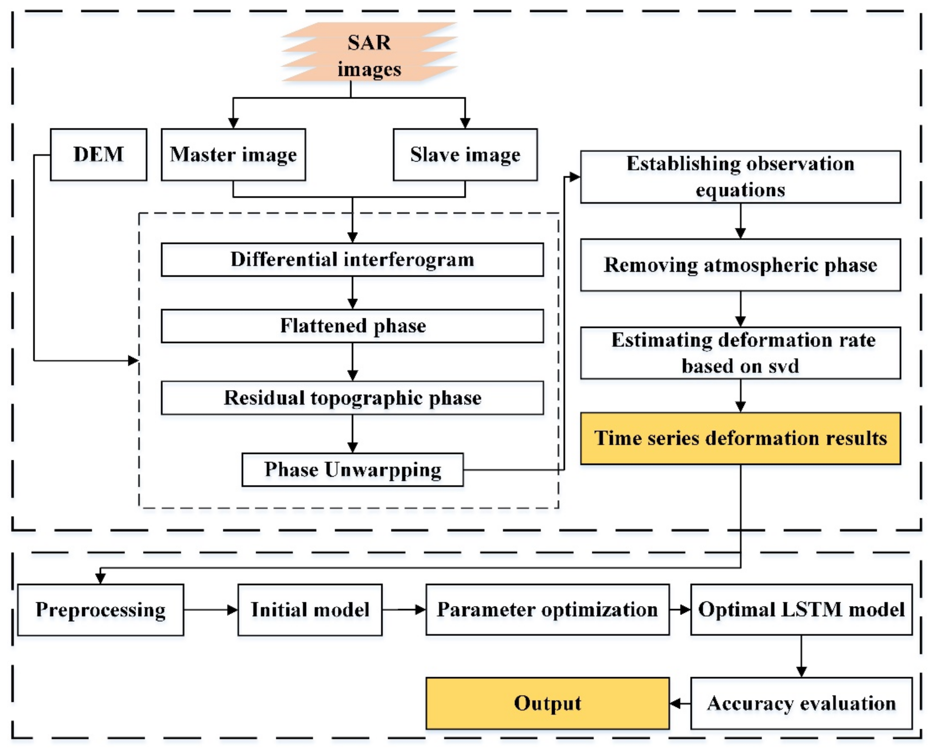
2. Methods
2.1. Principles of SBAS InSAR
2.2. Principles of LSTM
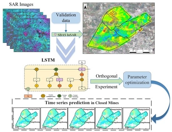
2.3. Time Series Prediction Model Combining SBAS InSAR Monitoring Results and LSTM
3. Case Study
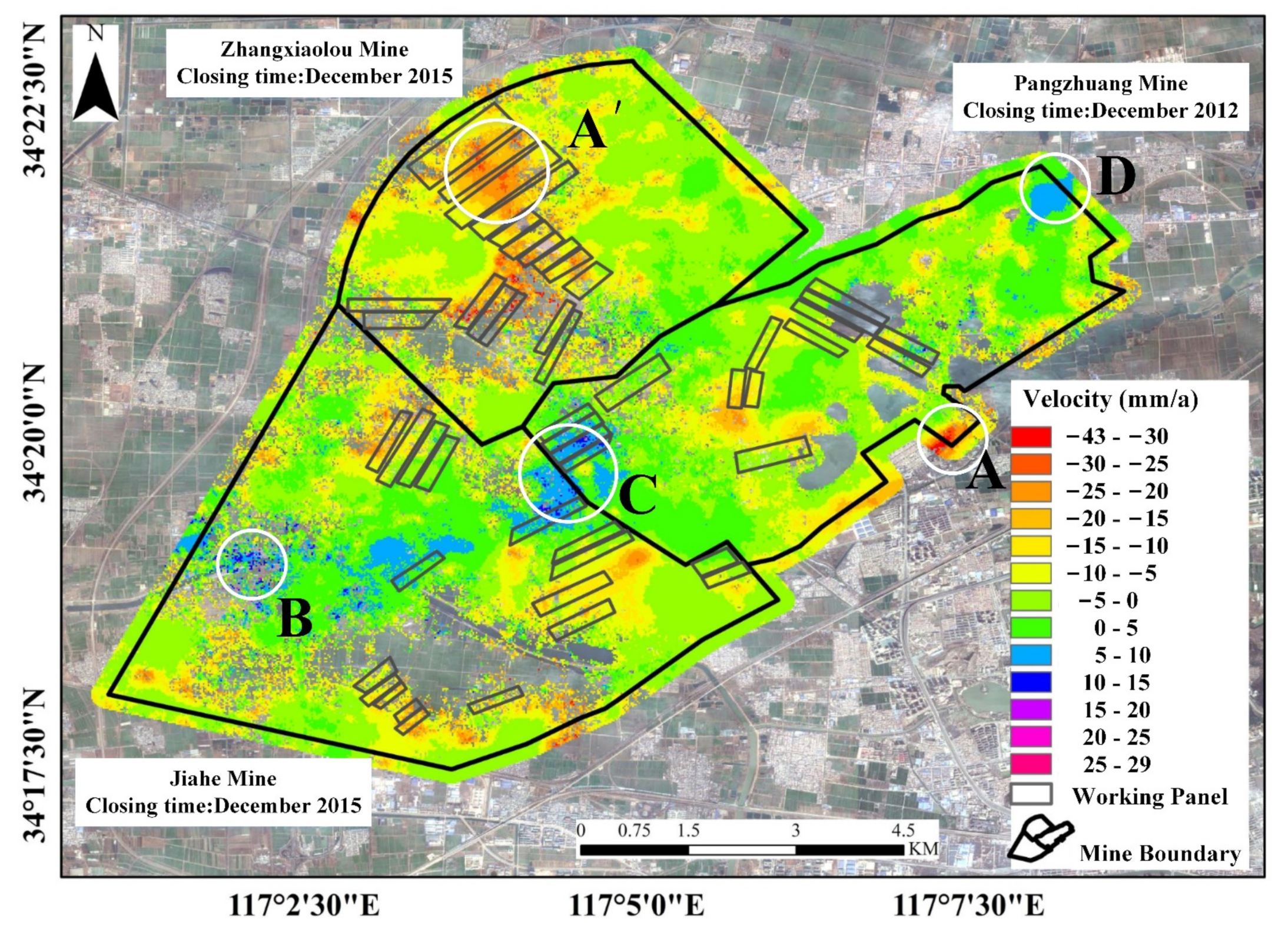
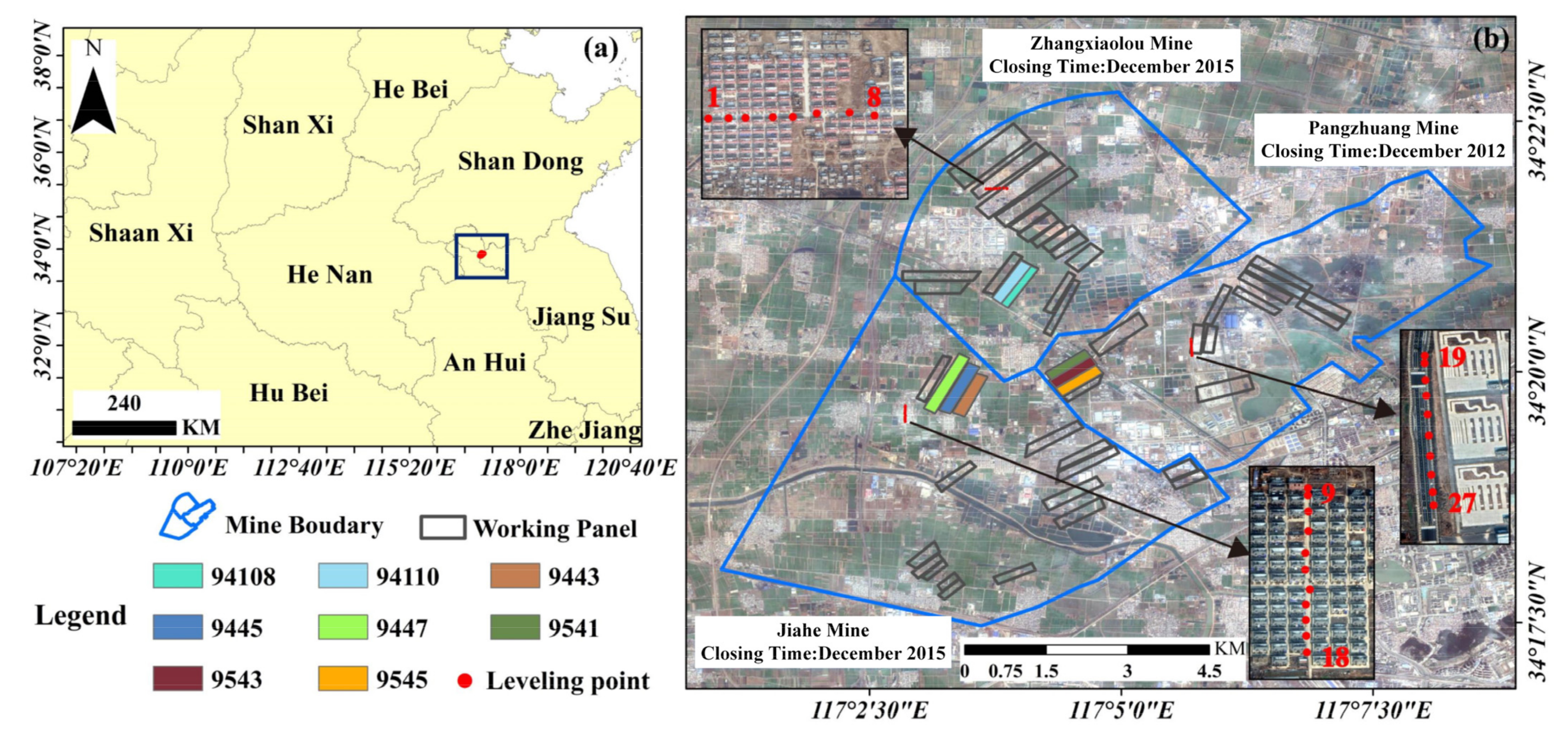
3.1. Study Area
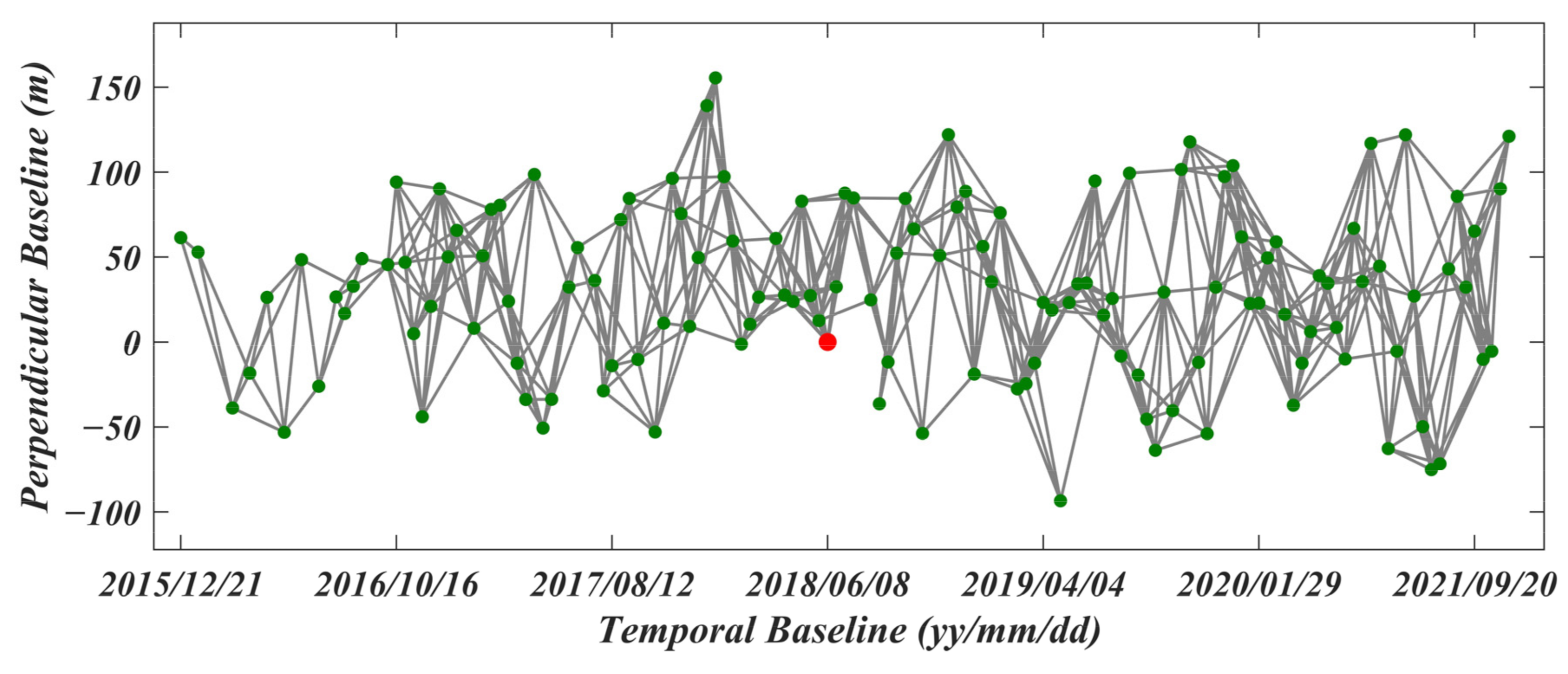
3.2. Data
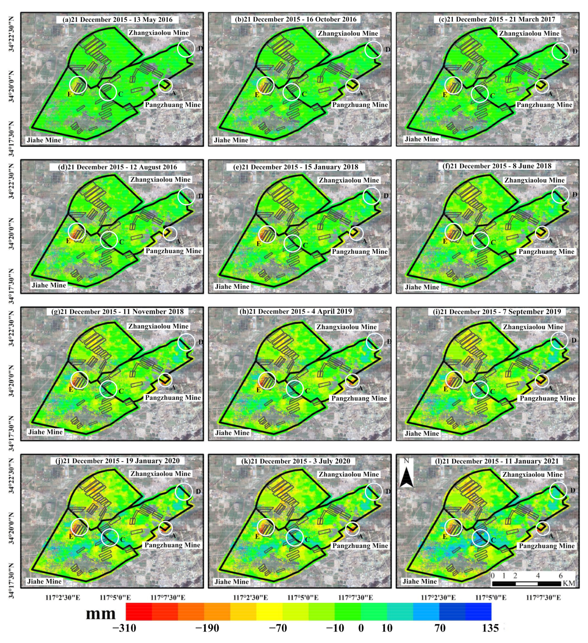
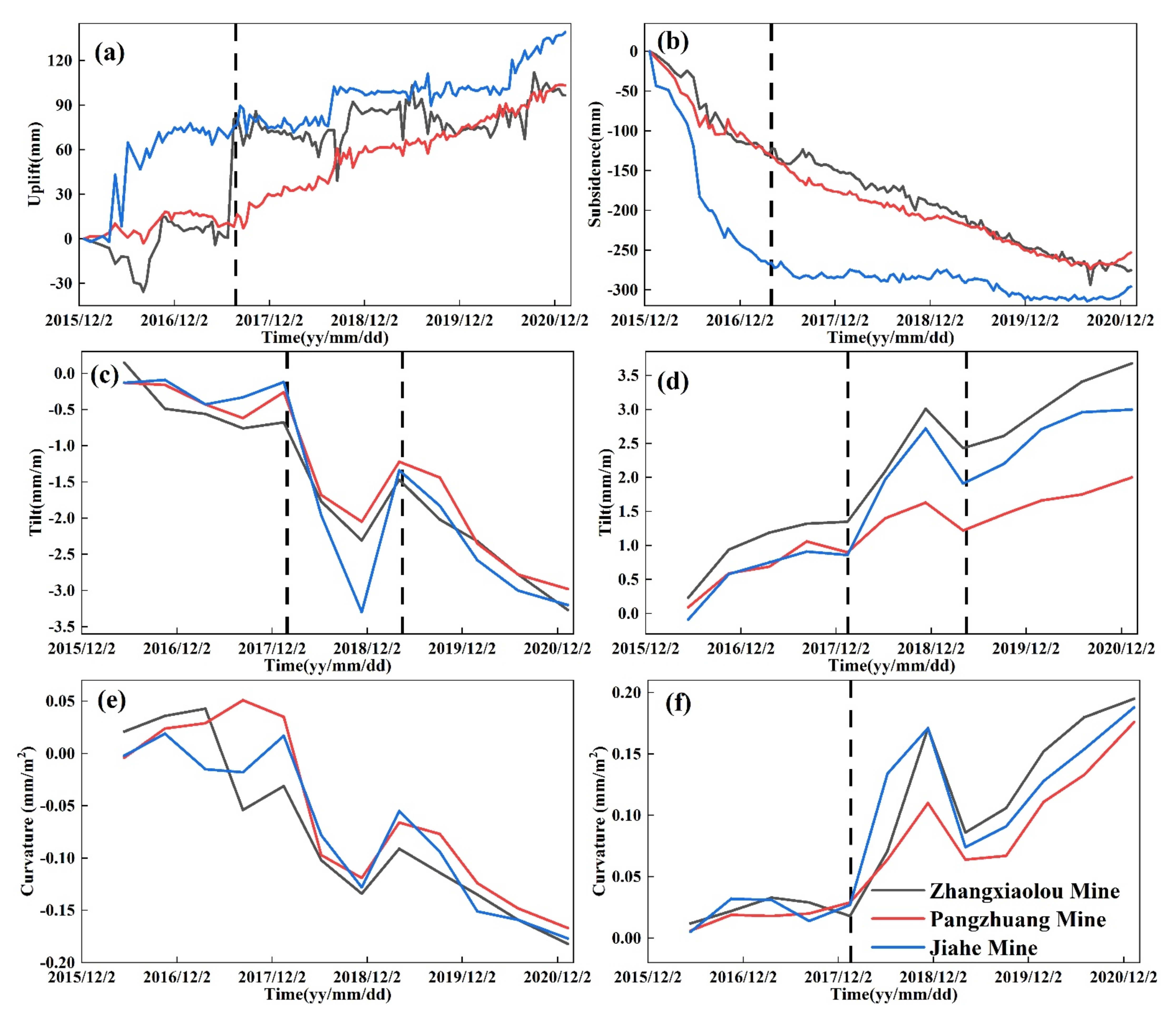
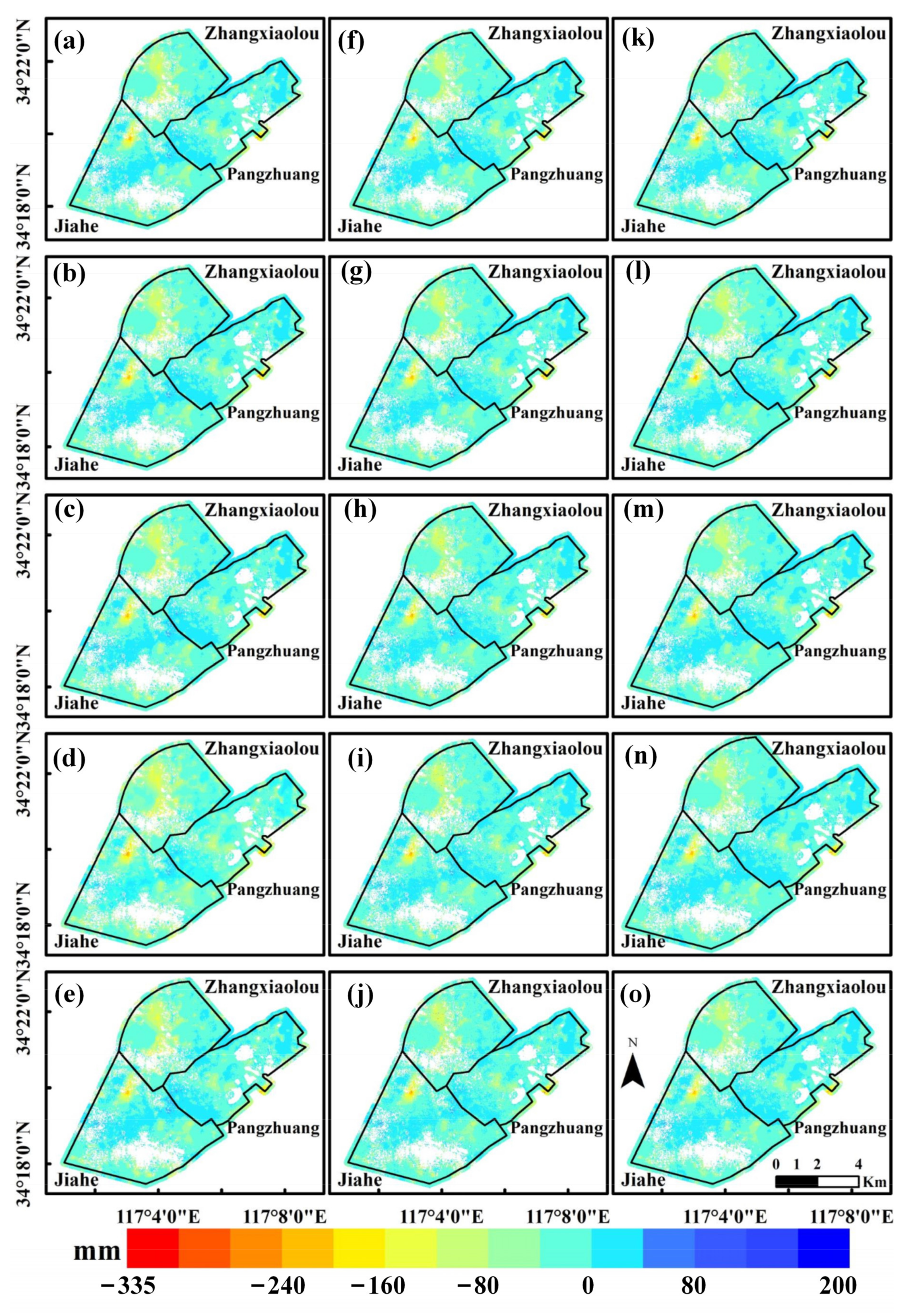
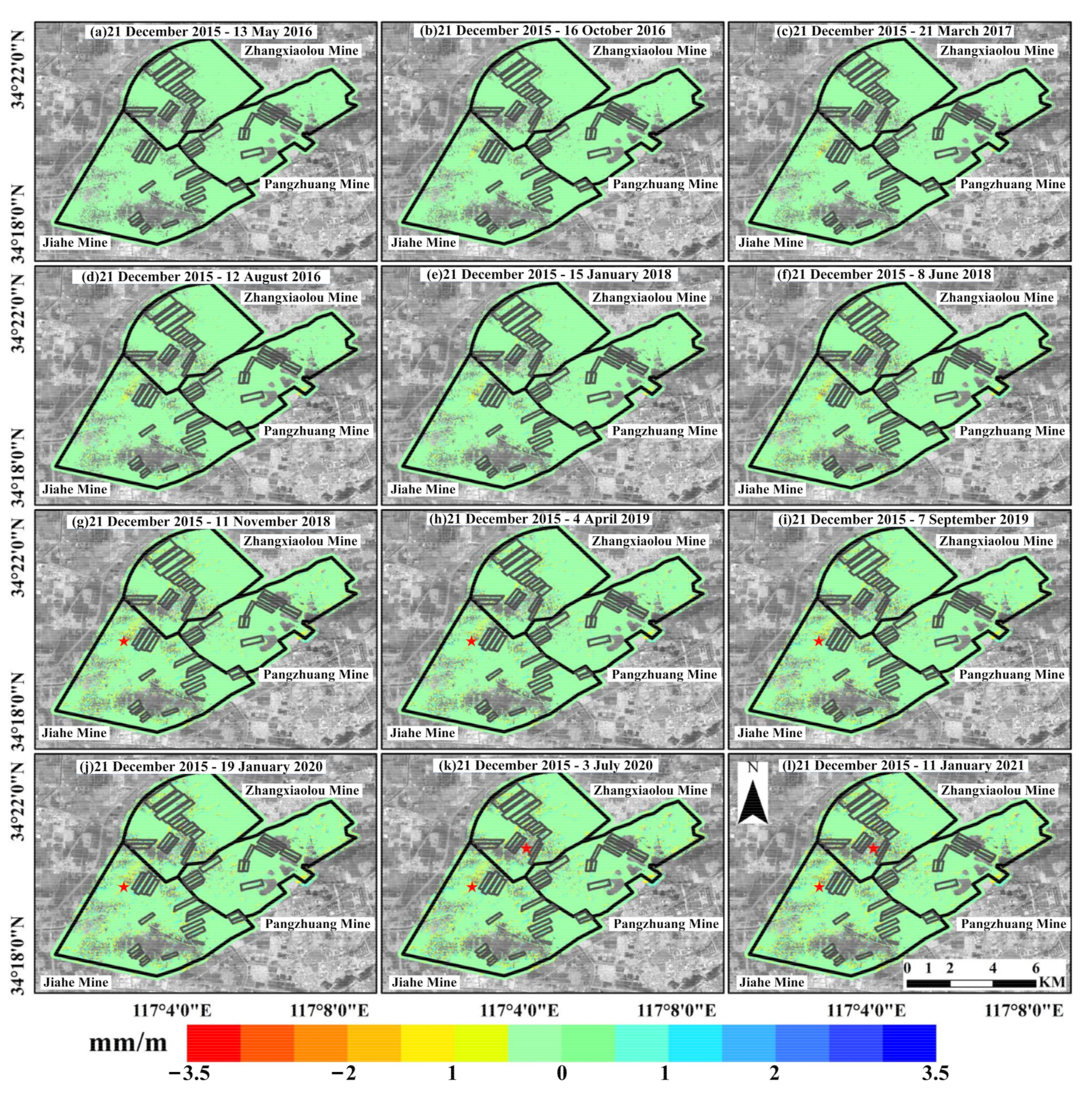
3.3. Analysis of Deformation Monitoring Results
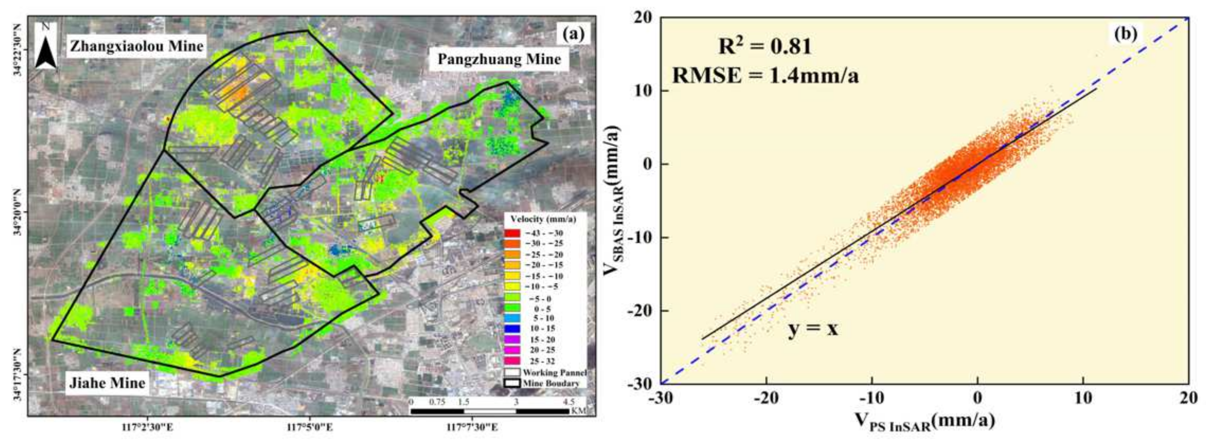
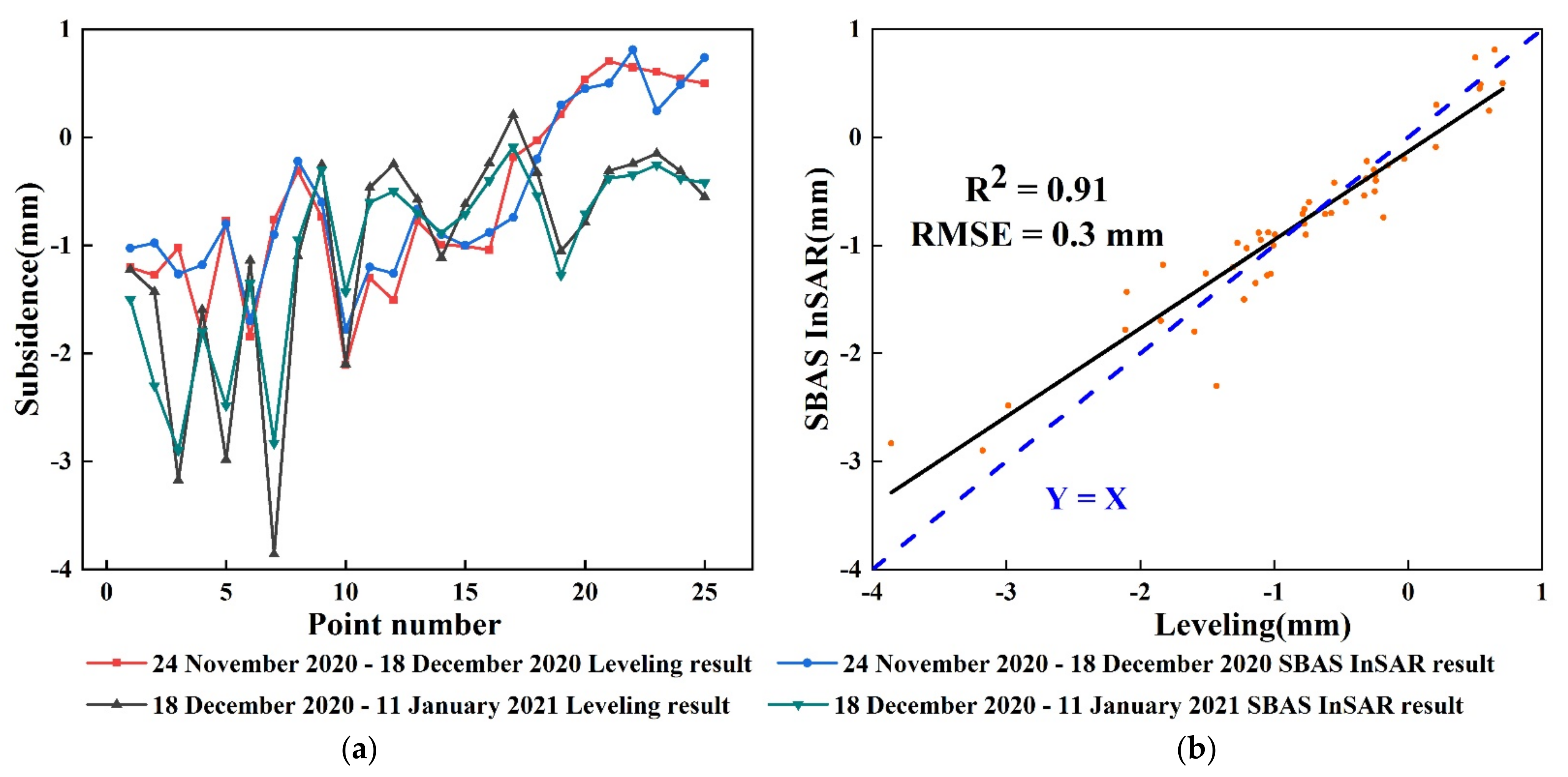
3.4. Data Accuracy Verification
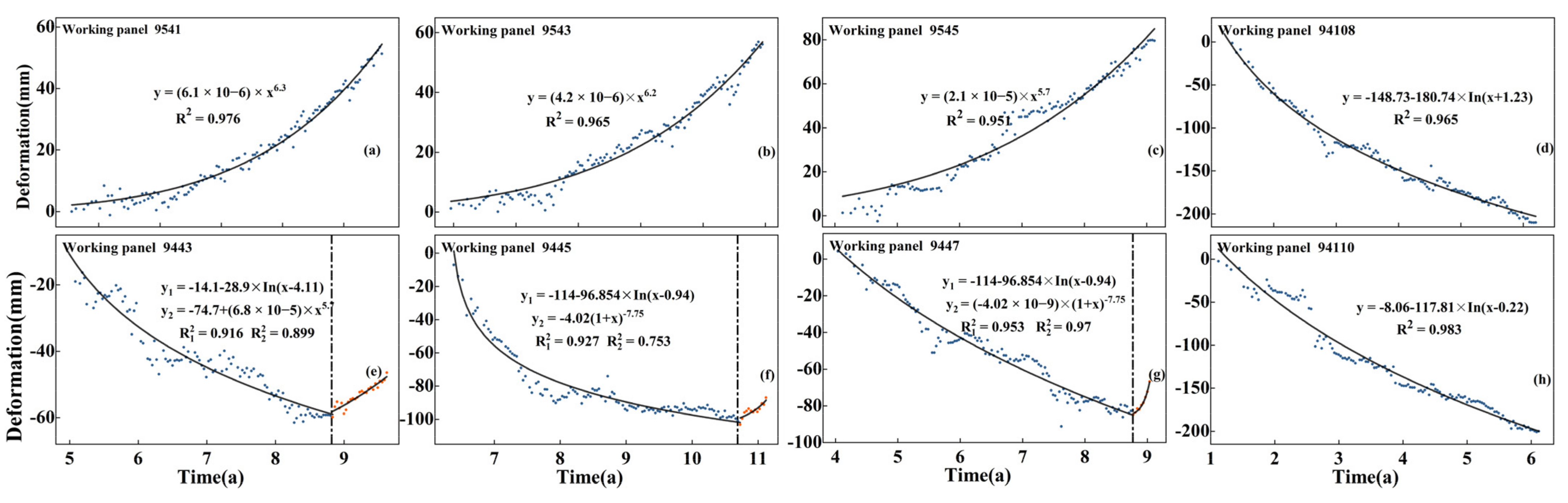
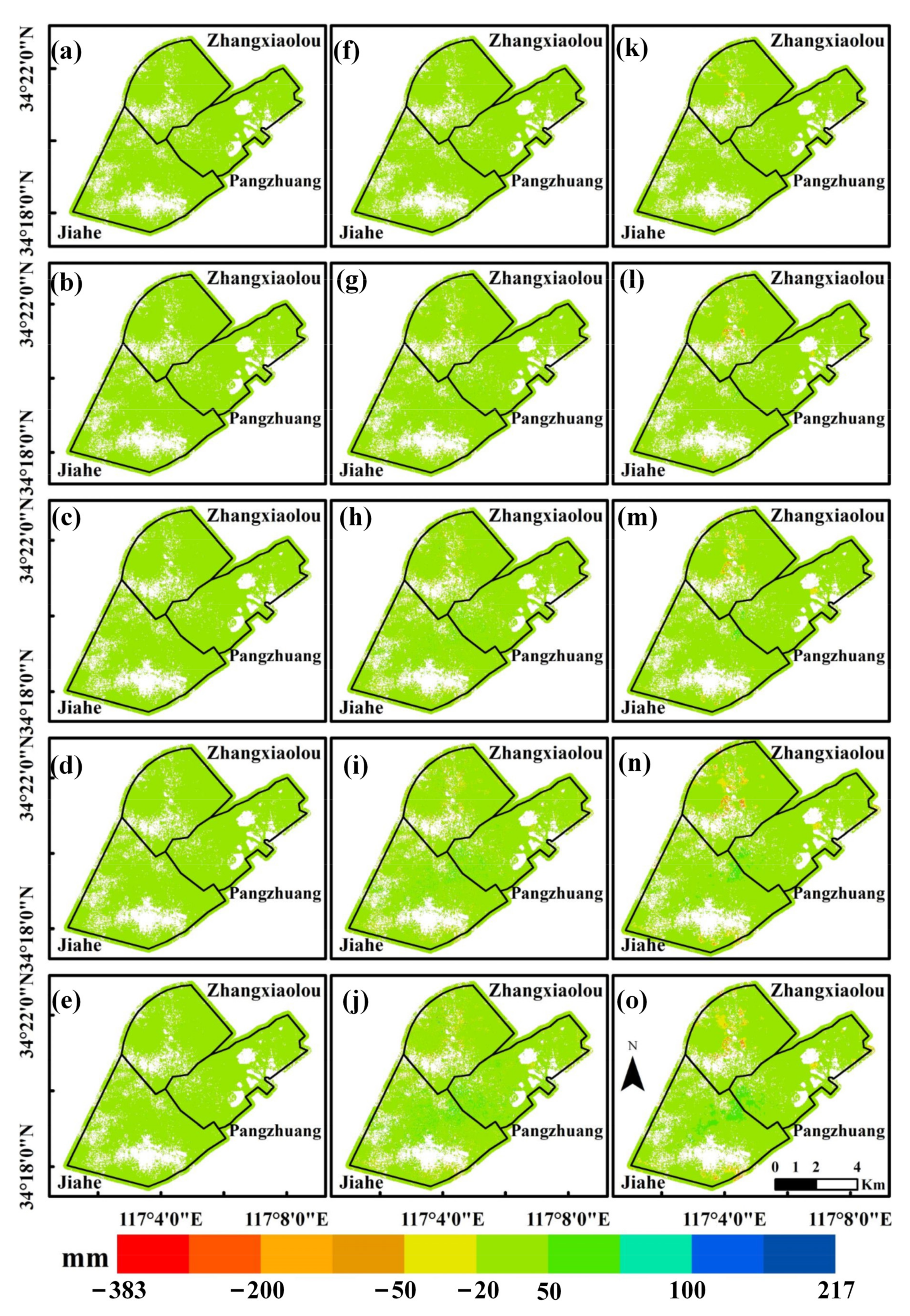
3.5. Subsidence Prediction Based on SBAS InSAR Results
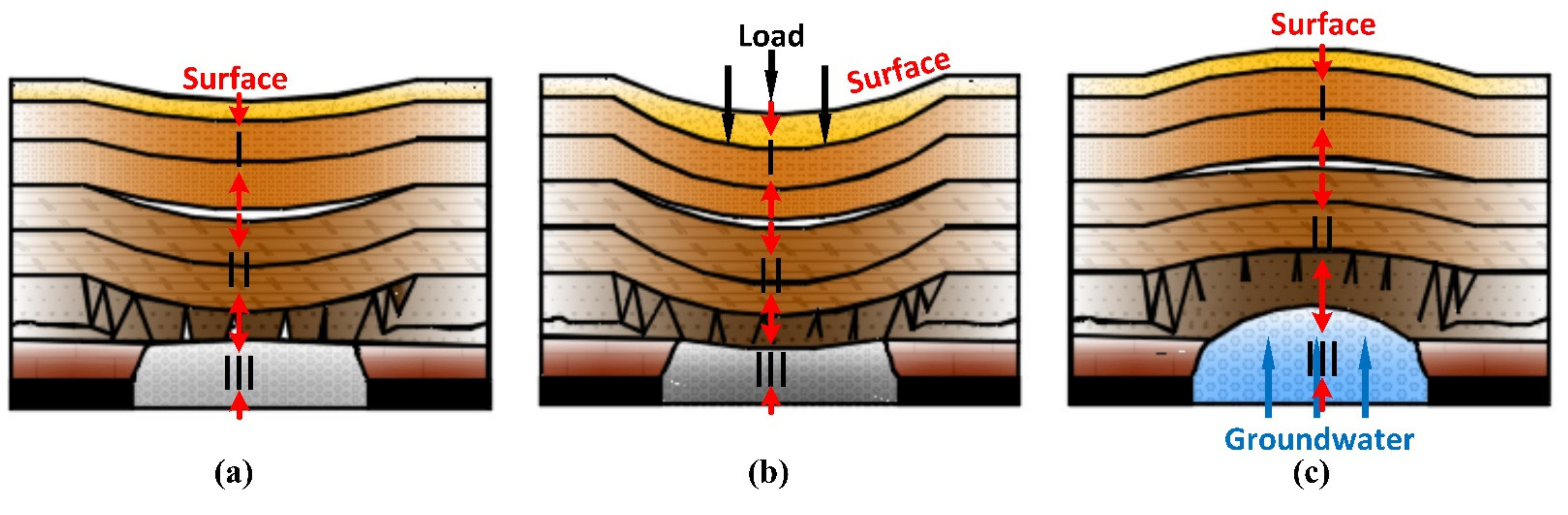
4. Discussion
5. Conclusions
Author Contributions
Funding
Institutional Review Board Statement
Informed Consent Statement
Data Availability Statement
Acknowledgments
Conflicts of Interest
References
- Fields, S. The earth’s open wounds: Abandoned and orphaned mines. Environ. Health Perspect. 2003, 111, A154–A161. [Google Scholar] [CrossRef] [Green Version]
- Unger, C.; Lechner, A.M.; Glenn, V.; Edraki, M.; Mulligan, D.R. Mapping and Prioritising Rehabilitation of Abandoned Mines in Australia. In Proceedings of the Life of Mine 2012, Maximising Mine Rehabilitation Outcomes, AusIMM/CMLR, Brisbane, Australia, 2012; The Australasian Institute of Mining and Metallurgy (AusIMM): Carlton North, VIC, Australia, 2012; pp. 259–266. [Google Scholar]
- Inventory of Closed Mining Waste Facilities (Updated January 2014). Available online: http://publications.environment-agency.gov.uk/ (accessed on 20 November 2017).
- Yan, L. How to transform abandoned coal mines into new ones? China Coal J. 2021, 8, 5. (In Chinese) [Google Scholar]
- Guéguen, Y.; Deffontaines, B.; Fruneau, B.; Al Heib, M.; de Michele, M.; Raucoules, D.; Guise, Y.; Planchenault, J. Monitoring residual mining subsidence of Nord/Pas-de-Calais coal basin from differential and Persistent Scatterer Interferometry (Northern France). J. Appl. Geophys. 2009, 69, 24–34. [Google Scholar] [CrossRef]
- Cuenca, M.C.; Hooper, A.J.; Hanssen, R.F. Surface deformation induced by water influx in the abandoned coal mines in Limburg, The Netherlands observed by satellite radar interferometry. J. Appl. Geophys. 2013, 88, 1–11. [Google Scholar] [CrossRef]
- Blachowski, J.; Kopeć, A.; Milczarek, W.; Owczarz, K. Evolution of Secondary Deformations Captured by Satellite Radar Interferometry: Case Study of an Abandoned Coal Basin in SW Poland. Sustainability 2019, 11, 884. [Google Scholar] [CrossRef] [Green Version]
- Zipf, R.K.; Mark, C. Design methods to control violent pillar failures in room-and-pillar mines. Trans. Inst. Min. Metall. Sect. A-Min. Ind. 1997, 106, A124–A132. [Google Scholar]
- Aydan, O. Crustal stress changes and characteristics of damage to geo-engineering structures induced by the Great East Japan Earthquake of 2011. Bull. Eng. Geol. Environ. 2015, 74, 1057–1070. [Google Scholar] [CrossRef]
- Chen, B.; Deng, K.; Fan, H.; Hao, M. Large-scale deformation monitoring in mining area by D-InSAR and 3D laser scanning technology integration. Int. J. Min. Sci. Technol. 2013, 23, 555–561. [Google Scholar] [CrossRef]
- Andrew, K.G.; Richard, M.G.; Howard, A.Z. Mapping small elevation changes over large areas: Differential radar interferometry. J. Geophys. Res. Solid Earth 1989, 94, 9183–9191. [Google Scholar] [CrossRef]
- Amelung, F.; Galloway, D.; Bell, J.W.; Zebker, H.A.; Laczniak, R.J. Sensing the ups and downs of Las Vegas: InSAR reveals structural control of land subsidence and aquifer-system deformation. Geology 1999, 27, 483–486. [Google Scholar] [CrossRef]
- Ferretti, A.; Prati, C.; Rocca, F. Nonlinear subsidence rate estimation using permanent scatterers in differential SAR interferometry. IEEE Trans. Geosci. Remote Sens. 2000, 38, 2202–2212. [Google Scholar] [CrossRef] [Green Version]
- Ferretti, A.; Prati, C.; Rocca, F. Permanent scatterers in SAR interferometry. IEEE Trans. Geosci. Remote Sens. 2001, 39, 8–20. [Google Scholar] [CrossRef]
- Berardino, P.; Fornaro, G.; Lanari, R.; Sansosti, E. A new algorithm for surface deformation monitoring based on small baseline differential SAR interferograms. IEEE Trans. Geosci. Remote Sens. 2002, 40, 2375–2383. [Google Scholar] [CrossRef] [Green Version]
- Chen, B.; Li, Z.; Yu, C.; Fairbairn, D.; Kang, J.; Hu, J.; Liang, L. Three-dimensional time-varying large surface displacements in coal exploiting areas revealed through integration of SAR pixel offset measurements and mining subsidence model. Remote Sens. Environ. 2020, 240, 111663. [Google Scholar] [CrossRef]
- Chen, B.; Mei, H.; Li, Z.; Wang, Z.; Yu, Y.; Yu, H. Retrieving Three-Dimensional Large Surface Displacements in Coal Mining Areas by Combining SAR Pixel Offset Measurements with an Improved Mining Subsidence Model. Remote Sens. 2021, 13, 2541. [Google Scholar] [CrossRef]
- Chen, B.; Deng, K.; Fan, H.; Yu, Y. Combining SAR interferometric phase and intensity information for monitoring of large gradient deformation in coal mining area. Eur. J. Remote Sens. 2015, 48, 701–717. [Google Scholar] [CrossRef] [Green Version]
- Zhao, C.-Y.; Zhang, Q.; Yang, C.; Zou, W. Integration of MODIS data and Short Baseline Subset (SBAS) technique for land subsidence monitoring in Datong, China. J. Geodyn. 2011, 52, 16–23. [Google Scholar] [CrossRef]
- Fan, H.; Xu, Q.; Hu, Z.; Du, S. Using temporarily coherent point interferometric synthetic aperture radar for land subsidence monitoring in a mining region of western China. J. Appl. Remote Sens. 2017, 11, 26003. [Google Scholar] [CrossRef]
- Dang, V.K.; Nguyen, T.D.; Dao, N.H.; Duong, T.L.; Dinh, X.V.; Weber, C. Land subsidence induced by underground coal mining at Quang Ninh, Vietnam: Persistent scatterer interferometric synthetic aperture radar observation using Sentinel-1 data. Int. J. Remote Sens. 2021, 42, 3563–3582. [Google Scholar] [CrossRef]
- Zhuang, N.; Yan, Y.; Chen, S.; Wang, H.; Shen, C. Multi-label learning based deep transfer neural network for facial attribute classification. Pattern Recognit. 2018, 80, 225–240. [Google Scholar] [CrossRef] [Green Version]
- Marcheggiani, D.; Titov, I. Encoding Sentences with Graph Convolutional Networks for Semantic Role Labeling. In Proceedings of the 2017 Conference on Empirical Methods in Natural Language Processing, Copenhagen, Denmark, 7–11 September 2017. [Google Scholar]
- Hinton, G.; Deng, L.; Yu, D.; Dahl, G.E.; Mohamed, A.-R.; Jaitly, N.; Senior, A.; Vanhoucke, V.; Nguyen, P.; Sainath, T.N.; et al. Deep Neural Networks for Acoustic Modeling in Speech Recognition: The Shared Views of Four Research Groups. IEEE Signal Process. Mag. 2012, 29, 82–97. [Google Scholar] [CrossRef]
- Rumelhart, D.E.; Hinton, G.E.; Williams, R.J. Learning representations by back-propagating errors. Nature 1986, 323, 533–536. [Google Scholar] [CrossRef]
- Gelenbe, E. Learning in the Recurrent Random Neural Network. Neural Comput. 1993, 5, 154–164. [Google Scholar] [CrossRef]
- Hochreiter, S.; Schmidhuber, J. Long short-term memory. Neural Comput. 1997, 9, 1735–1780. [Google Scholar] [CrossRef]
- Hanssen, R.F. Radar Interferometry: Data Interpretation and Error Analysis; Kluwer Academic: Dordrecht, The Netherlands, 2001. [Google Scholar]
- Gers, F.A.; Schmidhuber, J.; Cummins, F. Continual Prediction Using LSTM with Forget Gates; Springer: London, UK, 1999; pp. 133–138. [Google Scholar] [CrossRef]
- Schmidhuber, J. Gradient Flow in Recurrent Nets: The Difficulty of Learning Long-Term Dependencies; Wiley-IEEE Press: New York, NY, USA, 2001. [Google Scholar]
- Qing, X.; Niu, Y. Hourly day-ahead solar irradiance prediction using weather forecasts by LSTM. Energy 2018, 148, 461–468. [Google Scholar] [CrossRef]
- Li, Y.F.; Cao, H. Prediction for Tourism Flow based on LSTM Neural Network. Procedia Comput. Sci. 2018, 129, 277–283. [Google Scholar] [CrossRef]
- Kingma, D.; Ba, J. Adam: A Method for Stochastic Optimization. arXiv 2014, arXiv:1412.6980. [Google Scholar]
- Taguchi, G. Off-line and on-line quality control systems. In Proceedings of the International Conference on Quality, Tokyo, Japan, 6–12 September 1978; Volume 4, pp. 1–5. [Google Scholar]
- Fan, H.D.; Cheng, D.; Deng, K.Z.; Chen, B.Q.; Zhu, C.G. Subsidence monitoring using D-InSAR and probability integral prediction modelling in deep mining areas. Surv. Rev. 2015, 47, 438–445. [Google Scholar] [CrossRef]
- Zheng, M.; Zhang, H.; Deng, K.; Du, S.; Wang, L. Analysis of Pre- and Post-Mine Closure Surface Deformations in Western Xuzhou Coalfield From 2006 to 2018. IEEE Access 2019, 7, 124158–124172. [Google Scholar] [CrossRef]
- Costantini, M. A novel phase unwrapping method based on network programming. IEEE Trans. Geosci. Remote Sens. 1998, 36, 813–821. [Google Scholar] [CrossRef]
- Golub, G.H.; Loan, C. Matrix Computations: Matrix Computations; The Johns Hopkins University Press: Baltimore, MD, USA, 1996; pp. 49–79. [Google Scholar]
- Kratzsch, H. Mining Subsidence Engineering; Springer: Berlin/Heidelberg, Germany, 1983; pp. 62–89. [Google Scholar]
- State Bureau of Coal Industry. Regulations of Coal Pillar Design and Extraction for Buildings, Water Bodies Railways, Main Shafts and Roadways; Coal e Press: Beijing, China, 2000. (In Chinese) [Google Scholar]
- McKinley, S.; Levine, M. Cubic spline interpolation. Coll. Redw. 1998, 45, 1049–1060. [Google Scholar]
- Smola, A.J.; Schölkopf, B. A tutorial on support vector regression. Stat. Comput. 2004, 14, 199–222. [Google Scholar] [CrossRef] [Green Version]
- Palchik, V. Formation of fractured zones in overburden due to longwall mining. Environ. Earth Sci. 2003, 44, 28–38. [Google Scholar] [CrossRef]
- Peng, S.S.; Ma, W.M.; Zhong, W.L. Surface Subsidence Engineering; Society for Mining Metallurgy: New York, NY, USA, 1992; pp. 1–2. [Google Scholar]


| No. | Acquisition Date | Data Type | Perpendicular Baseline/m | Temporal Baseline/d |
|---|---|---|---|---|
| 1 | 21 December 2015 | SLC | 61.4 | 900 |
| 2 | 14 January 2016 | SLC | 52.9 | 876 |
| 3 | 2 March 2016 | SLC | −38.8 | 828 |
| 4 | 26 March 2016 | SLC | −18.3 | 804 |
| 5 | 19 April 2016 | SLC | 26.2 | 780 |
| 6 | 13 May 2016 | SLC | −53.1 | 756 |
| 7 | 6 June 2016 | SLC | 48.4 | 732 |
| 8 | 30 June 2016 | SLC | −26.1 | 708 |
| 9 | 24 July 2016 | SLC | 26.5 | 684 |
| 10 | 5 August 2016 | SLC | 16.7 | 672 |
| 11 | 17 August 2016 | SLC | 32.8 | 660 |
| 12 | 29 August 2016 | SLC | 49.0 | 648 |
| 13 | 4 October 2016 | SLC | 45.5 | 612 |
| 14 | 16 October 2016 | SLC | 94.2 | 600 |
| 59 | 8 June 2018 | SLC | 0 | 0 |
| 130 | 12 November 2020 | SLC | 32.3 | 888 |
| 131 | 24 November 2020 | SLC | 65.2 | 900 |
| 132 | 6 December 2020 | SLC | −10.2 | 912 |
| 133 | 18 December 2020 | SLC | −5.4 | 924 |
| 134 | 30 December 2020 | SLC | 90.2 | 936 |
| 135 | 11 January 2021 | SLC | 121.1 | 948 |
| Symbol | Factor | Level | |||
|---|---|---|---|---|---|
| 1 | 2 | 3 | 4 | ||
| A | Number of iterations | 100 | 200 | 300 | 400 |
| B | Number of hidden units | 100 | 200 | 300 | 400 |
| C | Learning rate | 0.001 | 0.0025 | 0.005 | 0.01 |
| D | Number of hidden layers | 1 | 2 | 3 | 4 |
| No. | Factor | RMSE (mm) | Time (s) | |||
|---|---|---|---|---|---|---|
| Iterations | Hidden Units | Learning Rate | Hidden Layers | |||
| 1 | 100 | 100 | 0.001 | 1 | 2.26 | 40.1 |
| 2 | 100 | 200 | 0.0025 | 2 | 2.02 | 59.5 |
| 3 | 100 | 300 | 0.005 | 3 | 2.87 | 81.6 |
| 4 | 100 | 400 | 0.01 | 4 | 6.3 | 137.5 |
| 5 | 200 | 100 | 0.0025 | 3 | 3.01 | 149.8 |
| 6 | 200 | 200 | 0.001 | 4 | 3.06 | 209.2 |
| 7 | 200 | 300 | 0.01 | 1 | 2.98 | 59.5 |
| 8 | 200 | 400 | 0.005 | 2 | 2.85 | 137.3 |
| 9 | 300 | 100 | 0.005 | 4 | 4.12 | 284.3 |
| 10 | 300 | 200 | 0.01 | 3 | 4.63 | 236.4 |
| 11 | 300 | 300 | 0.001 | 2 | 2.4 | 157.2 |
| 12 | 300 | 400 | 0.0025 | 1 | 2.38 | 105.1 |
| 13 | 400 | 100 | 0.01 | 2 | 3.97 | 205.3 |
| 14 | 400 | 200 | 0.005 | 1 | 3.25 | 122.4 |
| 15 | 400 | 300 | 0.0025 | 4 | 4.05 | 350.3 |
| 16 | 400 | 100 | 0.001 | 3 | 2.92 | 385.3 |
| Mine | Working Panel | Mining Termination Time | The Ratio of Mining Depth to Extraction Thickness | Length–Width Ratio of Working Panel |
|---|---|---|---|---|
| Pangzhuang Mine | 9541 | June 2008 | 315 | 5.56 |
| 9543 | February 2007 | 326 | 4.64 | |
| 9545 | December 2005 | 335 | 4.41 | |
| Jiahe Mine | 9443 | June 2011 | 435 | 7.31 |
| 9445 | December 2009 | 461 | 5.48 | |
| 9447 | January 2012 | 618 | 5.13 | |
| Zhangxiaolou Mine | 94110 | December 2014 | 585 | 4.85 |
| 94108 | November 2014 | 639 | 8.3 |
Publisher’s Note: MDPI stays neutral with regard to jurisdictional claims in published maps and institutional affiliations. |
© 2022 by the authors. Licensee MDPI, Basel, Switzerland. This article is an open access article distributed under the terms and conditions of the Creative Commons Attribution (CC BY) license (https://creativecommons.org/licenses/by/4.0/).
Share and Cite
Chen, B.; Yu, H.; Zhang, X.; Li, Z.; Kang, J.; Yu, Y.; Yang, J.; Qin, L. Time-Varying Surface Deformation Retrieval and Prediction in Closed Mines through Integration of SBAS InSAR Measurements and LSTM Algorithm. Remote Sens. 2022, 14, 788. https://doi.org/10.3390/rs14030788
Chen B, Yu H, Zhang X, Li Z, Kang J, Yu Y, Yang J, Qin L. Time-Varying Surface Deformation Retrieval and Prediction in Closed Mines through Integration of SBAS InSAR Measurements and LSTM Algorithm. Remote Sensing. 2022; 14(3):788. https://doi.org/10.3390/rs14030788
Chicago/Turabian StyleChen, Bingqian, Hao Yu, Xiang Zhang, Zhenhong Li, Jianrong Kang, Yang Yu, Jiale Yang, and Lu Qin. 2022. "Time-Varying Surface Deformation Retrieval and Prediction in Closed Mines through Integration of SBAS InSAR Measurements and LSTM Algorithm" Remote Sensing 14, no. 3: 788. https://doi.org/10.3390/rs14030788
APA StyleChen, B., Yu, H., Zhang, X., Li, Z., Kang, J., Yu, Y., Yang, J., & Qin, L. (2022). Time-Varying Surface Deformation Retrieval and Prediction in Closed Mines through Integration of SBAS InSAR Measurements and LSTM Algorithm. Remote Sensing, 14(3), 788. https://doi.org/10.3390/rs14030788