
The Role of Remote Sensing Data and Methods in a Modern Approach to Fertilization in Precision Agriculture


Abstract
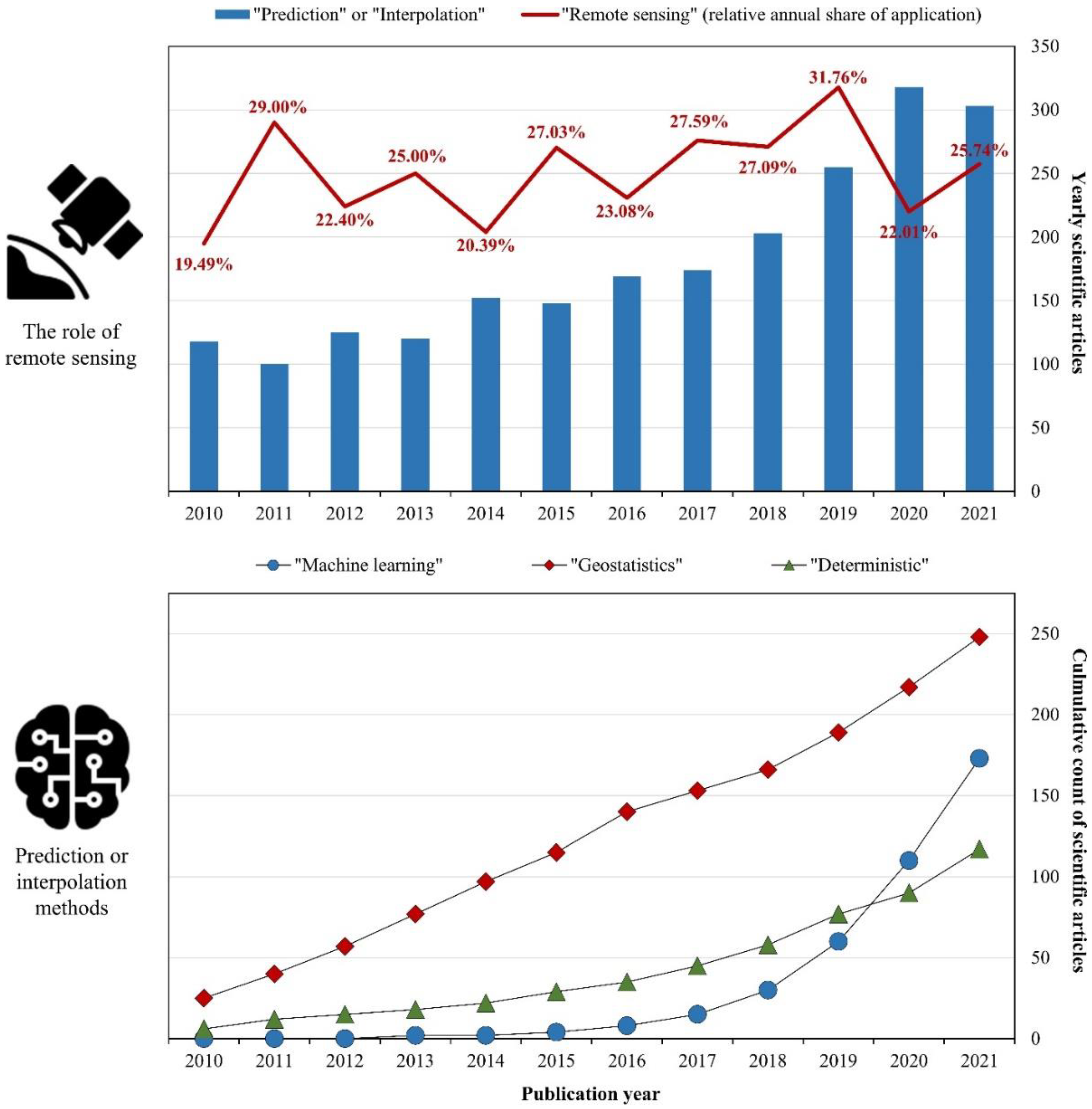
1. Introduction
2. Integration of Geoinformation Technologies with Agronomic Principles of Precision Fertilization
3. Conventional Approach to Fertilization in Precision Agriculture
3.1. Geostatistical Spatial Interpolation Methods
3.2. Deterministic Spatial Interpolation Methods
4. Modern Approach to Fertilization in Precision Agriculture
4.1. Remote Sensing Data
- (1)
- various indices for an improved description of the earth’s surface (e.g., water, vegetation, soil) based on multispectral images or
- (2)
- various derivatives of the digital elevation models such as slope, curvature, or flow accumulation analysis.
4.2. Modern Remote Sensing Methods for Optimal Fertilization in Precision Agriculture
- (1)
- Multivariate regressions based on various remote sensing data and
- (2)
- Machine and deep learning methods for predictions.
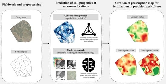
5. A Representative Overview of Modern and Conventional Approaches for Fertilization in Precision Agriculture
6. Conclusions
Author Contributions
Funding
Data Availability Statement
Acknowledgments
Conflicts of Interest
References
- Ray, D.K.; Ramankutty, N.; Mueller, N.D.; West, P.C.; Foley, J.A. Recent Patterns of Crop Yield Growth and Stagnation. Nat. Commun. 2012, 3, 1293. [Google Scholar] [CrossRef] [PubMed]
- Radočaj, D.; Jurišić, M.; Gašparović, M.; Plaščak, I.; Antonić, O. Cropland Suitability Assessment Using Satellite-Based Biophysical Vegetation Properties and Machine Learning. Agronomy 2021, 11, 1620. [Google Scholar] [CrossRef]
- Sela, S.; van Es, H.M.; Moebius-Clune, B.N.; Marjerison, R.; Kneubuhler, G. Dynamic Model-Based Recommendations Increase the Precision and Sustainability of N Fertilization in Midwestern US Maize Production. Comput. Electron. Agric. 2018, 153, 256–265. [Google Scholar] [CrossRef]
- Jurišić, M.; Radočaj, D.; Plaščak, I.; Rapčan, I. A Comparison of Precise Fertilization Prescription Rates to a Conventional Approach Based on the Open Source Gis Software. Poljoprivreda 2021, 27, 52–59. [Google Scholar] [CrossRef]
- Pogrzeba, M.; Rusinowski, S.; Krzyżak, J. Macroelements and Heavy Metals Content in Energy Crops Cultivated on Contaminated Soil under Different Fertilization—Case Studies on Autumn Harvest. Environ. Sci. Pollut. Res. 2018, 25, 12096–12106. [Google Scholar] [CrossRef]
- Bogunovic, I.; Pereira, P.; Brevik, E.C. Spatial Distribution of Soil Chemical Properties in an Organic Farm in Croatia. Sci. Total Environ. 2017, 584–585, 535–545. [Google Scholar] [CrossRef]
- Vizzari, M.; Santaga, F.; Benincasa, P. Sentinel 2-Based Nitrogen VRT Fertilization in Wheat: Comparison between Traditional and Simple Precision Practices. Agronomy 2019, 9, 278. [Google Scholar] [CrossRef]
- Zha, H.; Miao, Y.; Wang, T.; Li, Y.; Zhang, J.; Sun, W.; Feng, Z.; Kusnierek, K. Improving Unmanned Aerial Vehicle Remote Sensing-Based Rice Nitrogen Nutrition Index Prediction with Machine Learning. Remote Sens. 2020, 12, 215. [Google Scholar] [CrossRef]
- Lemaire, G.; Sinclair, T.; Sadras, V.; Bélanger, G. Allometric Approach to Crop Nutrition and Implications for Crop Diagnosis and Phenotyping. A Review. Agron. Sustain. Dev. 2019, 39, 27. [Google Scholar] [CrossRef]
- Nogueira Martins, R.; Magalhaes Valente, D.S.; Fim Rosas, J.T.; Souza Santos, F.; Lima Dos Santos, F.F.; Nascimento, M.; Campana Nascimento, A.C. Site-Specific Nutrient Management Zones in Soybean Field Using Multivariate Analysis: An Approach Based on Variable Rate Fertilization. Commun. Soil Sci. Plant Anal. 2020, 51, 687–700. [Google Scholar] [CrossRef]
- Zhang, L.; Yang, L.; Ma, T.; Shen, F.; Cai, Y.; Zhou, C. A Self-Training Semi-Supervised Machine Learning Method for Predictive Mapping of Soil Classes with Limited Sample Data. Geoderma 2021, 384, 114809. [Google Scholar] [CrossRef]
- Tu, J.; Yang, G.; Qi, P.; Ding, Z.; Mei, G. Comparative Investigation of Parallel Spatial Interpolation Algorithms for Building Large-Scale Digital Elevation Models. Peerj Comput. Sci. 2020, 6, e263. [Google Scholar] [CrossRef] [PubMed]
- Papadopoulos, A.; Kalivas, D.; Hatzichristos, T. GIS Modelling for Site-Specific Nitrogen Fertilization towards Soil Sustainability. Sustainability 2015, 7, 6684–6705. [Google Scholar] [CrossRef]
- Maes, W.H.; Steppe, K. Perspectives for Remote Sensing with Unmanned Aerial Vehicles in Precision Agriculture. Trends Plant Sci. 2019, 24, 152–164. [Google Scholar] [CrossRef] [PubMed]
- Lamb, D.W.; Brown, R.B. PA—Precision Agriculture: Remote-Sensing and Mapping of Weeds in Crops. J. Agric. Eng. Res. 2001, 78, 117–125. [Google Scholar] [CrossRef]
- Segarra, J.; Buchaillot, M.L.; Araus, J.L.; Kefauver, S.C. Remote Sensing for Precision Agriculture: Sentinel-2 Improved Features and Applications. Agronomy 2020, 10, 641. [Google Scholar] [CrossRef]
- Deng, L.; Mao, Z.; Li, X.; Hu, Z.; Duan, F.; Yan, Y. UAV-Based Multispectral Remote Sensing for Precision Agriculture: A Comparison between Different Cameras. ISPRS J. Photogramm. Remote Sens. 2018, 146, 124–136. [Google Scholar] [CrossRef]
- Xie, Q.; Dash, J.; Huete, A.; Jiang, A.; Yin, G.; Ding, Y.; Peng, D.; Hall, C.C.; Brown, L.; Shi, Y.; et al. Retrieval of Crop Biophysical Parameters from Sentinel-2 Remote Sensing Imagery. Int. J. Appl. Earth Obs. Geoinf. 2019, 80, 187–195. [Google Scholar] [CrossRef]
- Skakun, S.; Kalecinski, N.I.; Brown, M.G.L.; Johnson, D.M.; Vermote, E.F.; Roger, J.-C.; Franch, B. Assessing Within-Field Corn and Soybean Yield Variability from WorldView-3, Planet, Sentinel-2, and Landsat 8 Satellite Imagery. Remote Sens. 2021, 13, 872. [Google Scholar] [CrossRef]
- Aragon, B.; Houborg, R.; Tu, K.; Fisher, J.B.; McCabe, M. CubeSats Enable High Spatiotemporal Retrievals of Crop-Water Use for Precision Agriculture. Remote Sens. 2018, 10, 1867. [Google Scholar] [CrossRef]
- Houborg, R.; McCabe, M.F. High-Resolution NDVI from Planet’s Constellation of Earth Observing Nano-Satellites: A New Data Source for Precision Agriculture. Remote Sens. 2016, 8, 768. [Google Scholar] [CrossRef]
- Gašparović, M.; Zrinjski, M.; Barković, Đ.; Radočaj, D. An Automatic Method for Weed Mapping in Oat Fields Based on UAV Imagery. Comput. Electron. Agric. 2020, 173, 105385. [Google Scholar] [CrossRef]
- De Castro, A.I.; Torres-Sánchez, J.; Peña, J.M.; Jiménez-Brenes, F.M.; Csillik, O.; López-Granados, F. An Automatic Random Forest-OBIA Algorithm for Early Weed Mapping between and within Crop Rows Using UAV Imagery. Remote Sens. 2018, 10, 285. [Google Scholar] [CrossRef]
- Chlingaryan, A.; Sukkarieh, S.; Whelan, B. Machine Learning Approaches for Crop Yield Prediction and Nitrogen Status Estimation in Precision Agriculture: A Review. Comput. Electron. Agric. 2018, 151, 61–69. [Google Scholar] [CrossRef]
- Danner, M.; Berger, K.; Wocher, M.; Mauser, W.; Hank, T. Efficient RTM-Based Training of Machine Learning Regression Algorithms to Quantify Biophysical & Biochemical Traits of Agricultural Crops. ISPRS J. Photogramm. Remote Sens. 2021, 173, 278–296. [Google Scholar] [CrossRef]
- Jimenez, A.F.; Ortiz, B.; Bondesan, L.; Morata, G.; Damianidis, D. Evaluation of Two Recurrent Neural Network Methods for Prediction of Irrigation Rate and Timing. Trans. Asabe 2020, 63, 1327–1348. [Google Scholar] [CrossRef]
- Bhatt, R.; Sanjay-Swami. Soil Fertility Status of Ratte Khera Farm of Punjab Agricultural University, Punjab, India. J. Environ. Biol. 2020, 41, 1665–1675. [Google Scholar] [CrossRef]
- De Zorzi, P.; Barbizzi, S.; Belli, M.; Mufato, R.; Sartori, G.; Stocchero, G. Soil Sampling Strategies: Evaluation of Different Approaches. Appl. Radiat. Isot. 2008, 66, 1691–1694. [Google Scholar] [CrossRef]
- Radočaj, D.; Jug, I.; Vukadinović, V.; Jurišić, M.; Gašparović, M. The Effect of Soil Sampling Density and Spatial Autocorrelation on Interpolation Accuracy of Chemical Soil Properties in Arable Cropland. Agronomy 2021, 11, 2430. [Google Scholar] [CrossRef]
- Dong, W.; Wu, T.; Luo, J.; Sun, Y.; Xia, L. Land Parcel-Based Digital Soil Mapping of Soil Nutrient Properties in an Alluvial-Diluvia Plain Agricultural Area in China. Geoderma 2019, 340, 234–248. [Google Scholar] [CrossRef]
- Gia Pham, T.; Kappas, M.; Van Huynh, C.; Hoang Khanh Nguyen, L. Application of Ordinary Kriging and Regression Kriging Method for Soil Properties Mapping in Hilly Region of Central Vietnam. ISPRS Int. J. Geo-Inf. 2019, 8, 147. [Google Scholar] [CrossRef]
- Šiljeg, A.; Lozić, S.; Šiljeg, S. The Accuracy of Deterministic Models of Interpolation in the Process of Generating a Digital Terrain Model—The Example of the Vrana Lake Nature Park. Teh. Vjesn.-Tech. Gaz. 2015, 22, 853–863. [Google Scholar] [CrossRef][Green Version]
- Mirás-Avalos, J.M.; Fandiño, M.; Rey, B.J.; Dafonte, J.; Cancela, J.J. Zoning of a Newly-Planted Vineyard: Spatial Variability of Physico-Chemical Soil Properties. Soil Syst. 2020, 4, 62. [Google Scholar] [CrossRef]
- Shaddad, S.M.; Buttafuoco, G.; Castrignanò, A. Assessment and Mapping of Soil Salinization Risk in an Egyptian Field Using a Probabilistic Approach. Agronomy 2020, 10, 85. [Google Scholar] [CrossRef]
- Hengl, T. Finding the Right Pixel Size. Comput. Geosci. 2006, 32, 1283–1298. [Google Scholar] [CrossRef]
- Liu, Y.; Chen, Y.; Wu, Z.; Wang, B.; Wang, S. Geographical Detector-Based Stratified Regression Kriging Strategy for Mapping Soil Organic Carbon with High Spatial Heterogeneity. Catena 2021, 196, 104953. [Google Scholar] [CrossRef]
- Chen, S.; Arrouays, D.; Leatitia Mulder, V.; Poggio, L.; Minasny, B.; Roudier, P.; Libohova, Z.; Lagacherie, P.; Shi, Z.; Hannam, J.; et al. Digital Mapping of GlobalSoilMap Soil Properties at a Broad Scale: A Review. Geoderma 2022, 409, 115567. [Google Scholar] [CrossRef]
- Song, X.-D.; Liu, F.; Wu, H.-Y.; Cao, Q.; Zhong, C.; Yang, J.-L.; Li, D.-C.; Zhao, Y.-G.; Zhang, G.-L. Effects of Long-Term K Fertilization on Soil Available Potassium in East China. Catena 2020, 188, 104412. [Google Scholar] [CrossRef]
- Román Dobarco, M.; Orton, T.G.; Arrouays, D.; Lemercier, B.; Paroissien, J.-B.; Walter, C.; Saby, N.P.A. Prediction of Soil Texture Using Descriptive Statistics and Area-to-Point Kriging in Region Centre (France). Geoderma Reg. 2016, 7, 279–292. [Google Scholar] [CrossRef]
- Dad, J.M.; Shafiq, M.U. Spatial Distribution of Soil Organic Carbon in Apple Orchard Soils of Kashmir Himalaya, India. Carbon Manag. 2021, 12, 485–498. [Google Scholar] [CrossRef]
- Zhang, J.; Wang, Y.; Qu, M.; Chen, J.; Yang, L.; Huang, B.; Zhao, Y. Source Apportionment of Soil Nitrogen and Phosphorus Based on Robust Residual Kriging and Auxiliary Soil-Type Map in Jintan County, China. Ecol. Indic. 2020, 119, 106820. [Google Scholar] [CrossRef]
- Della Chiesa, S.; Genova, G.; la Cecilia, D.; Niedrist, G. Phytoavailable Phosphorus (P2O5) and Potassium (K2O) in Topsoil for Apple Orchards and Vineyards, South Tyrol, Italy. J. Maps 2019, 15, 555–562. [Google Scholar] [CrossRef]
- Bogunovic, I.; Kisic, I.; Mesic, M.; Percin, A.; Zgorelec, Z.; Bilandžija, D.; Jonjic, A.; Pereira, P. Reducing Sampling Intensity in Order to Investigate Spatial Variability of Soil PH, Organic Matter and Available Phosphorus Using Co-Kriging Techniques. A Case Study of Acid Soils in Eastern Croatia. Arch. Agron. Soil Sci. 2017, 63, 1852–1863. [Google Scholar] [CrossRef]
- Wang, Y.; Xiao, Z.; Aurangzeib, M.; Zhang, X.; Zhang, S. Effects of Freeze-Thaw Cycles on the Spatial Distribution of Soil Total Nitrogen Using a Geographically Weighted Regression Kriging Method. Sci. Total Environ. 2021, 763, 142993. [Google Scholar] [CrossRef] [PubMed]
- Sidorova, V.A.; Zhukovskii, E.E.; Lekomtsev, P.V.; Yakushev, V.V. Geostatistical Analysis of the Soil and Crop Parameters in a Field Experiment on Precision Agriculture. Eurasian Soil Sci. 2012, 45, 783–792. [Google Scholar] [CrossRef]
- Nourzadeh, M.; Mahdian, M.H.; Malakouti, M.J.; Khavazi, K. Investigation and Prediction Spatial Variability in Chemical Properties of Agricultural Soil Using Geostatistics. Arch. Agron. Soil Sci. 2012, 58, 461–475. [Google Scholar] [CrossRef]
- Radočaj, D.; Jurišić, M.; Antonić, O. Determination of Soil C:N Suitability Zones for Organic Farming Using an Unsupervised Classification in Eastern Croatia. Ecol. Indic. 2021, 123, 107382. [Google Scholar] [CrossRef]
- Attorre, F.; Alfo, M.; De Sanctis, M.; Francesconi, F.; Bruno, F. Comparison of Interpolation Methods for Mapping Climatic and Bioclimatic Variables at Regional Scale. Int. J. Climatol. 2007, 27, 1825–1843. [Google Scholar] [CrossRef]
- Wang, W.; Cai, L.; Peng, P.; Gong, Y.; Yang, X. Soil Sampling Spacing Based on Precision Agriculture Variable Rate Fertilization of Pomegranate Orchard. Commun. Soil Sci. Plant Anal. 2021, 52, 2445–2461. [Google Scholar] [CrossRef]
- Betzek, N.M.; de Souza, E.G.; Bazzi, C.L.; Schenatto, K.; Gavioli, A.; Graziano Magalhaes, P.S. Computational Routines for the Automatic Selection of the Best Parameters Used by Interpolation Methods to Create Thematic Maps. Comput. Electron. Agric. 2019, 157, 49–62. [Google Scholar] [CrossRef]
- Tziachris, P.; Metaxa, E.; Papadopoulos, F.; Papadopoulou, M. Spatial Modelling and Prediction Assessment of Soil Iron Using Kriging Interpolation with PH as Auxiliary Information. ISPRS Int. J. Geo-Inf. 2017, 6, 283. [Google Scholar] [CrossRef]
- Xu, Y.; Wang, X.; Bai, J.; Wang, D.; Wang, W.; Guan, Y. Estimating the Spatial Distribution of Soil Total Nitrogen and Available Potassium in Coastal Wetland Soils in the Yellow River Delta by Incorporating Multi-Source Data. Ecol. Indic. 2020, 111, 106002. [Google Scholar] [CrossRef]
- Dash, P.K.; Panigrahi, N.; Mishra, A. Identifying Opportunities to Improve Digital Soil Mapping in India: A Systematic Review. Geoderma Reg. 2022, 28, e00478. [Google Scholar] [CrossRef]
- Ploner, A.; Dutter, R. New Directions in Geostatistics. J. Stat. Plan. Inference 2000, 91, 499–509. [Google Scholar] [CrossRef]
- Oliver, M.A.; Webster, R. A Tutorial Guide to Geostatistics: Computing and Modelling Variograms and Kriging. Catena 2014, 113, 56–69. [Google Scholar] [CrossRef]
- Wang, K.; Zhang, C.; Li, W. Comparison of Geographically Weighted Regression and Regression Kriging for Estimating the Spatial Distribution of Soil Organic Matter. GIScience Remote Sens. 2012, 49, 915–932. [Google Scholar] [CrossRef]
- Jurišić, M.; Radočaj, D.; Krčmar, S.; Plaščak, I.; Gašparović, M. Geostatistical Analysis of Soil C/N Deficiency and Its Effect on Agricultural Land Management of Major Crops in Eastern Croatia. Agronomy 2020, 10, 1996. [Google Scholar] [CrossRef]
- Pardo-Iguzquiza, E.; Dowd, P.A. Comparison of Inference Methods for Estimating Semivariogram Model Parameters and Their Uncertainty: The Case of Small Data Sets. Comput. Geosci. 2013, 50, 154–164. [Google Scholar] [CrossRef]
- Australia Government. A Review of Spatial Interpolation Methods for Environmental Scientists; Geoscience Australia: Canberra, Australia, 2008.
- Robinson, T.P.; Metternicht, G. Testing the Performance of Spatial Interpolation Techniques for Mapping Soil Properties. Comput. Electron. Agric. 2006, 50, 97–108. [Google Scholar] [CrossRef]
- Bărbulescu, A.; Șerban, C.; Indrecan, M.-L. Computing the Beta Parameter in IDW Interpolation by Using a Genetic Algorithm. Water 2021, 13, 863. [Google Scholar] [CrossRef]
- Xie, Y.; Chen, T.; Lei, M.; Yang, J.; Guo, Q.; Song, B.; Zhou, X. Spatial Distribution of Soil Heavy Metal Pollution Estimated by Different Interpolation Methods: Accuracy and Uncertainty Analysis. Chemosphere 2011, 82, 468–476. [Google Scholar] [CrossRef] [PubMed]
- Voltz, M.; Webster, R. A Comparison of Kriging, Cubic Splines and Classification for Predicting Soil Properties from Sample Information. J. Soil Sci. 1990, 41, 473–490. [Google Scholar] [CrossRef]
- Bahri, F.M.Z.; Sharples, J.J. Sensitivity of the Empirical Mode Decomposition to Interpolation Methodology and Data Non-Stationarity. Environ. Model. Assess. 2019, 24, 437–456. [Google Scholar] [CrossRef]
- Hengl, T.; de Jesus, J.M.; MacMillan, R.A.; Batjes, N.H.; Heuvelink, G.B.M.; Ribeiro, E.; Samuel-Rosa, A.; Kempen, B.; Leenaars, J.G.B.; Walsh, M.G.; et al. SoilGrids1km—Global Soil Information Based on Automated Mapping. PLoS ONE 2014, 9, e105992. [Google Scholar] [CrossRef] [PubMed]
- Hengl, T.; de Jesus, J.M.; Heuvelink, G.B.M.; Gonzalez, M.R.; Kilibarda, M.; Blagotić, A.; Shangguan, W.; Wright, M.N.; Geng, X.; Bauer-Marschallinger, B.; et al. SoilGrids250m: Global Gridded Soil Information Based on Machine Learning. PLoS ONE 2017, 12, e0169748. [Google Scholar] [CrossRef] [PubMed]
- Nussbaum, M.; Spiess, K.; Baltensweiler, A.; Grob, U.; Keller, A.; Greiner, L.; Schaepman, M.E.; Papritz, A. Evaluation of Digital Soil Mapping Approaches with Large Sets of Environmental Covariates. SOIL 2018, 4, 1–22. [Google Scholar] [CrossRef]
- Sun, X.-L.; Wang, Y.; Wang, H.-L.; Zhang, C.; Wang, Z.-L. Digital Soil Mapping Based on Empirical Mode Decomposition Components of Environmental Covariates. Eur. J. Soil Sci. 2019, 70, 1109–1127. [Google Scholar] [CrossRef]
- Shahbazi, F.; Hughes, P.; McBratney, A.B.; Minasny, B.; Malone, B.P. Evaluating the Spatial and Vertical Distribution of Agriculturally Important Nutrients—Nitrogen, Phosphorous and Boron—In North West Iran. Catena 2019, 173, 71–82. [Google Scholar] [CrossRef]
- Fathololoumi, S.; Vaezi, A.R.; Alavipanah, S.K.; Ghorbani, A.; Saurette, D.; Biswas, A. Improved Digital Soil Mapping with Multitemporal Remotely Sensed Satellite Data Fusion: A Case Study in Iran. Sci. Total Environ. 2020, 721, 137703. [Google Scholar] [CrossRef]
- John, K.; Abraham Isong, I.; Michael Kebonye, N.; Okon Ayito, E.; Chapman Agyeman, P.; Marcus Afu, S. Using Machine Learning Algorithms to Estimate Soil Organic Carbon Variability with Environmental Variables and Soil Nutrient Indicators in an Alluvial Soil. Land 2020, 9, 487. [Google Scholar] [CrossRef]
- Hengl, T.; Miller, M.A.E.; Križan, J.; Shepherd, K.D.; Sila, A.; Kilibarda, M.; Antonijević, O.; Glušica, L.; Dobermann, A.; Haefele, S.M.; et al. African Soil Properties and Nutrients Mapped at 30 m Spatial Resolution Using Two-Scale Ensemble Machine Learning. Sci. Rep. 2021, 11, 6130. [Google Scholar] [CrossRef] [PubMed]
- Poggio, L.; de Sousa, L.M.; Batjes, N.H.; Heuvelink, G.B.M.; Kempen, B.; Ribeiro, E.; Rossiter, D. SoilGrids 2.0: Producing Soil Information for the Globe with Quantified Spatial Uncertainty. SOIL 2021, 7, 217–240. [Google Scholar] [CrossRef]
- Guo, L.; Sun, X.; Fu, P.; Shi, T.; Dang, L.; Chen, Y.; Linderman, M.; Zhang, G.; Zhang, Y.; Jiang, Q.; et al. Mapping Soil Organic Carbon Stock by Hyperspectral and Time-Series Multispectral Remote Sensing Images in Low-Relief Agricultural Areas. Geoderma 2021, 398, 115118. [Google Scholar] [CrossRef]
- Zhang, Z.; Ding, J.; Zhu, C.; Chen, X.; Wang, J.; Han, L.; Ma, X.; Xu, D. Bivariate Empirical Mode Decomposition of the Spatial Variation in the Soil Organic Matter Content: A Case Study from NW China. Catena 2021, 206, 105572. [Google Scholar] [CrossRef]
- Radocaj, D.; Obhodas, J.; Jurisic, M.; Gasparovic, M. Global Open Data Remote Sensing Satellite Missions for Land Monitoring and Conservation: A Review. Land 2020, 9, 402. [Google Scholar] [CrossRef]
- Gasparović, M.; Dobrinić, D. Comparative Assessment of Machine Learning Methods for Urban Vegetation Mapping Using Multitemporal Sentinel-1 Imagery. Remote Sens. 2020, 12, 1952. [Google Scholar] [CrossRef]
- El Hajj, M.; Baghdadi, N.; Zribi, M.; Bazzi, H. Synergic Use of Sentinel-1 and Sentinel-2 Images for Operational Soil Moisture Mapping at High Spatial Resolution over Agricultural Areas. Remote Sens. 2017, 9, 1292. [Google Scholar] [CrossRef]
- Uddin, K.; Matin, M.A.; Meyer, F.J. Operational Flood Mapping Using Multi-Temporal Sentinel-1 SAR Images: A Case Study from Bangladesh. Remote Sens. 2019, 11, 1581. [Google Scholar] [CrossRef]
- Gasparovic, M.; Klobucar, D. Mapping Floods in Lowland Forest Using Sentinel-1 and Sentinel-2 Data and an Object-Based Approach. Forests 2021, 12, 553. [Google Scholar] [CrossRef]
- Balenzano, A.; Mattia, F.; Satalino, G.; Lovergine, F.P.; Palmisano, D.; Peng, J.; Marzahn, P.; Wegmuller, U.; Cartus, O.; Dabrowska-Zielinska, K.; et al. Sentinel-1 Soil Moisture at 1 Km Resolution: A Validation Study. Remote Sens. Environ. 2021, 263, 112554. [Google Scholar] [CrossRef]
- Zeraatpisheh, M.; Garosi, Y.; Reza Owliaie, H.; Ayoubi, S.; Taghizadeh-Mehrjardi, R.; Scholten, T.; Xu, M. Improving the Spatial Prediction of Soil Organic Carbon Using Environmental Covariates Selection: A Comparison of a Group of Environmental Covariates. CATENA 2022, 208, 105723. [Google Scholar] [CrossRef]
- Erler, A.; Riebe, D.; Beitz, T.; Loehmannsroeben, H.-G.; Gebbers, R. Soil Nutrient Detection for Precision Agriculture Using Handheld Laser-Induced Breakdown Spectroscopy (LIBS) and Multivariate Regression Methods (PLSR, Lasso and GPR). Sensors 2020, 20, 418. [Google Scholar] [CrossRef] [PubMed]
- Das, K.; Twarakavi, N.; Khiripet, N.; Chattanrassamee, P.; Kijkullert, C. A Machine Learning Framework for Mapping Soil Nutrients with Multi-Source Data Fusion. In Proceedings of the 2021 IEEE International Geoscience and Remote Sensing Symposium IGARSS, Brussels, Belgium, 11–16 July 2021; pp. 3705–3708. [Google Scholar]
- Qiu, Z.; Ma, F.; Li, Z.; Xu, X.; Ge, H.; Du, C. Estimation of Nitrogen Nutrition Index in Rice from UAV RGB Images Coupled with Machine Learning Algorithms. Comput. Electron. Agric. 2021, 189, 106421. [Google Scholar] [CrossRef]
- Selige, T.; Boehner, J.; Schmidhalter, U. High Resolution Topsoil Mapping Using Hyperspectral Image and Field Data in Multivariate Regression Modeling Procedures. Geoderma 2006, 136, 235–244. [Google Scholar] [CrossRef]
- Paustian, M.; Theuvsen, L. Adoption of Precision Agriculture Technologies by German Crop Farmers. Precis. Agric. 2017, 18, 701–716. [Google Scholar] [CrossRef]
- Zhang, L.; Zhang, L.; Du, B. Deep Learning for Remote Sensing Data A Technical Tutorial on the State of the Art. IEEE Geosci. Remote Sens. Mag. 2016, 4, 22–40. [Google Scholar] [CrossRef]
- Lary, D.J.; Alavi, A.H.; Gandomi, A.H.; Walker, A.L. Machine Learning in Geosciences and Remote Sensing. Geosci. Front. 2016, 7, 3–10. [Google Scholar] [CrossRef]
- Zhu, X.X.; Tuia, D.; Mou, L.; Xia, G.-S.; Zhang, L.; Xu, F.; Fraundorfer, F. Deep Learning in Remote Sensing: A Comprehensive Review and List of Resources. IEEE Geosci. Remote Sens. Mag. 2017, 5, 8–36. [Google Scholar] [CrossRef]
- Maxwell, A.E.; Warner, T.A.; Fang, F. Implementation of Machine-Learning Classification in Remote Sensing: An Applied Review. Int. J. Remote Sens. 2018, 39, 2784–2817. [Google Scholar] [CrossRef]
- Chatziantoniou, A.; Petropoulos, G.P.; Psomiadis, E. Co-Orbital Sentinel 1 and 2 for LULC Mapping with Emphasis on Wetlands in a Mediterranean Setting Based on Machine Learning. Remote Sens. 2017, 9, 1259. [Google Scholar] [CrossRef]
- Zhang, C.; Sargent, I.; Pan, X.; Li, H.; Gardiner, A.; Hare, J.; Atkinson, P.M. Joint Deep Learning for Land Cover and Land Use Classification. Remote Sens. Environ. 2019, 221, 173–187. [Google Scholar] [CrossRef]
- Sibanda, M.; Mutanga, O.; Rouget, M. Examining the Potential of Sentinel-2 MSI Spectral Resolution in Quantifying above Ground Biomass across Different Fertilizer Treatments. ISPRS J. Photogramm. Remote Sens. 2015, 110, 55–65. [Google Scholar] [CrossRef]
- Basso, B.; Fiorentino, C.; Cammarano, D.; Schulthess, U. Variable Rate Nitrogen Fertilizer Response in Wheat Using Remote Sensing. Precis. Agric. 2016, 17, 168–182. [Google Scholar] [CrossRef]
- Ge, Y.; Zhang, J.; Zhang, L.; Yang, M.; He, J. Long-Term Fertilization Regimes Affect Bacterial Community Structure and Diversity of an Agricultural Soil in Northern China. J. Soils Sediments 2008, 8, 43–50. [Google Scholar] [CrossRef]
- Ye, H.; Lu, C.; Lin, Q. Investigation of the Spatial Heterogeneity of Soil Microbial Biomass Carbon and Nitrogen under Long-Term Fertilizations in Fluvo-Aquic Soil. PLoS ONE 2019, 14, e0209635. [Google Scholar] [CrossRef]
- Hengl, T.; MacMillan, R.A. Predictive Soil Mapping with R.; OpenGeoHub Foundation: Wageningen, The Netherlands, 2019; ISBN 978-0-359-30635-0. [Google Scholar]
- Olaya, V. Chapter 6 Basic Land-Surface Parameters. In Developments in Soil Science; Geomorphometry; Hengl, T., Reuter, H.I., Eds.; Elsevier: Amsterdam, The Netherlands, 2009; Volume 33, pp. 141–169. [Google Scholar]
- Freeman, T.G. Calculating Catchment Area with Divergent Flow Based on a Regular Grid. Comput. Geosci. 1991, 17, 413–422. [Google Scholar] [CrossRef]
- Conrad, O.; Bechtel, B.; Bock, M.; Dietrich, H.; Fischer, E.; Gerlitz, L.; Wehberg, J.; Wichmann, V.; Boehner, J. System for Automated Geoscientific Analyses (SAGA) v. 2.1.4. Geosci. Model Dev. 2015, 8, 1991–2007. [Google Scholar] [CrossRef]
- Rouse, J.; Haas, R.H.; Schell, J.A.; Deering, D.W. Monitoring Vegetation Systems in the Great Plains with ERTS. NASA Spec. Publ. 1974, 351, 309. [Google Scholar]
- Huete, A.; Didan, K.; Miura, T.; Rodriguez, E.P.; Gao, X.; Ferreira, L.G. Overview of the Radiometric and Biophysical Performance of the MODIS Vegetation Indices. Remote Sens. Environ. 2002, 83, 195–213. [Google Scholar] [CrossRef]
- Hunt, E.R.; Cavigelli, M.; Daughtry, C.S.T.; Mcmurtrey, J.E.; Walthall, C.L. Evaluation of Digital Photography from Model Aircraft for Remote Sensing of Crop Biomass and Nitrogen Status. Precis. Agric. 2005, 6, 359–378. [Google Scholar] [CrossRef]
- Deng, Y.; Wu, C.; Li, M.; Chen, R. RNDSI: A Ratio Normalized Difference Soil Index for Remote Sensing of Urban/Suburban Environments. Int. J. Appl. Earth Obs. Geoinf. 2015, 39, 40–48. [Google Scholar] [CrossRef]
- Escadafal, R. Remote Sensing of Arid Soil Surface Color with Landsat Thematic Mapper. Adv. Space Res. 1989, 9, 159–163. [Google Scholar] [CrossRef]
- Jin, S.; Sader, S.A. Comparison of Time Series Tasseled Cap Wetness and the Normalized Difference Moisture Index in Detecting Forest Disturbances. Remote Sens. Environ. 2005, 94, 364–372. [Google Scholar] [CrossRef]


| Selected Soil Properties | Number of Samples (Study Area) | Country | Conventional Methods | R2 Accuracy Range | Reference |
|---|---|---|---|---|---|
| potassium | 4266 (2,190,000 km2) | China | kriging with external drift | 0.247–0.290 | [38] |
| clay, silt, sand | 1842 (34,151 km2) | France | CK, RK | 0.460–0.780 (RK) 0.440–0.710 (CK) | [39] |
| SOC, pH, EC, bulk density | 1044 (15,948 km2) | India | OK, IDW, EBK | 0.928–0.941 (OK) 0.712–0.773 (IDW) | [40] |
| total nitrogen, phosphorous | 259 (975 km2) | China | OK, RK | 0.570–0.700 (RK) 0.510–0.680 (OK) | [41] |
| phosphorous, potassium | 16,000 (245 km2) | Italy | OK | 0.300–0.320 | [42] |
| SOC | 242 (141 km2) | China | OK, RK | 0.166–0.263 (RK) 0.004–0.142 (OK) | [36] |
| pH, phosphorous, SOM | 1004 (80.8 km2) | Croatia | IDW, OK, CK, spline | 0.533–0.689 (OK) 0.504–0.672 (IDW) | [43] |
| phosphorous, potassium | 160 (8.2 km2) | Croatia | OK, IDW | 0.759–0.794 (IDW) 0.713–0.743 (OK) | [29] |
| total nitrogen | 912 (1.9 km2) | China | GWR | 0.670–0.925 | [44] |
| phosphorous, potassium | 296 (1.2 km2) | Croatia | OK, IDW | 0.631–0.733 (OK) 0.400–0.693 (IDW) | [4] |
| pH, CEC, clay, EC, phosphorous, potassium | 149 (0.2 km2) | Spain | OK | 0.089–0.596 | [33] |
| pH, EC, SOM, phosphorous, potassium | 66 (0.003 km2) | Egypt | IK, PK | 0.706 (PK) 0.533 (IK) | [34] |
| Soil Properties | Prediction Methods | Multispectral/ Hyperspectral Images | DEM/ Radar Images | Reference |
|---|---|---|---|---|
| SOC, pH, sand, silt, clay, bulk density, CEC, coarse fragments | regression kriging, multiple linear regression, multinomial logistic regression | MODIS | SRTM | [65] |
| SOC, pH, sand, silt, clay, bulk density, CEC, coarse fragments | random forest, gradient boosting, neural networks | MODIS | SRTM | [66] |
| clay, silt, gravel, pH, SOM, bulk density, effective CEC | random forest, boosted regression trees | Landsat 7, SPOT5 | custom DEM | [67] |
| SOC, pH, clay, CEC | multiple linear regression, regression kriging | / | custom DEM | [68] |
| nitrogen, phosphorous, boron | random forest, cubist model | Landsat 8 | custom DEM | [69] |
| SOM, pH, SOC, total nitrogen, phosphorous, potassium | random forest, artificial neural network, co-kriging | GF-2 | SRTM | [30] |
| SOC, sand, CCE | random forest, cubist model | Landsat 8 | Alos AW3D | [70] |
| SOC | random forest, artificial neural networks, multiple linear regression | Landsat 8 | ASTER | [71] |
| SOC, sand, silt, clay, pH, calcium, potassium, nitrogen, phosphorous, etc. | two-scale ensemble machine learning | Sentinel-2, Landsat 8, MODIS, PROBA-V, SM2RAIN | Sentinel-1, AW3D | [72] |
| SOC, total nitrogen, pH, sand, silt, clay, bulk density, CEC, coarse fragments | recursive feature elimination, quantile random forest | Landsat 8, MODIS | EarthEnv-DEM90 | [73] |
| SOC, bulk density | partial least square regression, extreme learning machine | Sentinel-2, Landsat 8, Headwall-Hyperspec | / | [74] |
| SOM | random forest | Sentinel-2 | custom DEM | [75] |
| Soil Property | Average (mg 100 g–1) | Value Range (mg 100 g–1) | CV | SK | KT | Shapiro–Wilk Test | Moran’s I | |
|---|---|---|---|---|---|---|---|---|
| W | p | |||||||
| phosphorous pentoxide (P2O5) | 23.2 | 8.9–41.0 | 0.364 | 0.587 | –0.592 | 0.941 | 0.0005 | 0.209 |
| potassium oxide (K2O) | 26.1 | 17.2–50.5 | 0.253 | 1.517 | 3.092 | 0.877 | < 0.0001 | 0.124 |
| Data Source | Environmental Segment | Covariate | Reference |
|---|---|---|---|
| digital elevation model (EU-DEM v1.1) | morphometry | slope | [99] |
| aspect | |||
| total curvature | |||
| convergence index | |||
| hydrology | flow accumulation | [100] | |
| topographic wetness index | [101] | ||
| multispectral satellite images (Landsat 8, sensed on 15th September 2021) | vegetation | normalized difference vegetation index (NDVI) | [102] |
| enhanced vegetation index (EVI) | [103] | ||
| normalized green-red vegetation index (NGRDI) | [104] | ||
| soil | normalized difference soil index (NDSI) | [105] | |
| brightness index (BI) | [106] | ||
| moisture | normalized difference moisture index (NDMI) | [107] |
Publisher’s Note: MDPI stays neutral with regard to jurisdictional claims in published maps and institutional affiliations. |
© 2022 by the authors. Licensee MDPI, Basel, Switzerland. This article is an open access article distributed under the terms and conditions of the Creative Commons Attribution (CC BY) license (https://creativecommons.org/licenses/by/4.0/).
Share and Cite
Radočaj, D.; Jurišić, M.; Gašparović, M. The Role of Remote Sensing Data and Methods in a Modern Approach to Fertilization in Precision Agriculture. Remote Sens. 2022, 14, 778. https://doi.org/10.3390/rs14030778
Radočaj D, Jurišić M, Gašparović M. The Role of Remote Sensing Data and Methods in a Modern Approach to Fertilization in Precision Agriculture. Remote Sensing. 2022; 14(3):778. https://doi.org/10.3390/rs14030778
Chicago/Turabian StyleRadočaj, Dorijan, Mladen Jurišić, and Mateo Gašparović. 2022. "The Role of Remote Sensing Data and Methods in a Modern Approach to Fertilization in Precision Agriculture" Remote Sensing 14, no. 3: 778. https://doi.org/10.3390/rs14030778
APA StyleRadočaj, D., Jurišić, M., & Gašparović, M. (2022). The Role of Remote Sensing Data and Methods in a Modern Approach to Fertilization in Precision Agriculture. Remote Sensing, 14(3), 778. https://doi.org/10.3390/rs14030778