Marine Mixed Layer Height Detection Using Ship-Borne Coherent Doppler Wind Lidar Based on Constant Turbulence Threshold

Abstract

Marine mixed layer height (MLH) detection using a ship-borne coherent Doppler wind lidar (CDWL) based on a constant turbulent kinetic energy dissipation rate (TKEDR) threshold is realized and experimentally demonstrated. The MLH can be retrieved from the TKEDR estimated by the CDWL via setting an appropriate threshold. Here, the value of threshold is determined by a reference MLH retrieved from aerosol backscattered signal. The threshold of 10⁻⁴ m² s⁻³ is found to be applicable in retrieving both inland and marine MLHs. In the experiments, to validate the reliability of the constant threshold, the MLH diurnal cycles at inland and marine sites are retrieved by using a ground-based CDWL. The MLH retrieval result at the marine site shows good agreement with radiosonde-derived MLH. After that, by using a ship-borne CDWL, the marine MLH along the ship’s route in South China Sea is successfully detected in real time.

1. Introduction

The mixed layer (ML), also known as the convective boundary layer, is the lower part of the atmospheric boundary layer (ABL) which is directly influenced by the Earth’s surface and responds to surface forcing with a timescale of about an hour [1]. Mixed layer height (MLH) is defined as the height of ML top. Below the ML top, the heat, moisture, pollutants, and small gas constituents are mixed in the vertical. Therefore, the MLH is one of the key parameters in the boundary layer parameterization of weather and air quality models [2,3]. In particular, the marine ML is important to marine low cloud process and material exchange between the ocean and low atmosphere; thus, the marine MLH is critical to successful climate simulation [4] and accurate air–sea surface flux parameterization [5].

The material mixing in the ML is driven by convective turbulence; thus, the MLH can be retrieved from turbulence intensity, which is usually characterized by the vertical wind velocity variance or turbulent kinetic energy dissipation rate (TKEDR). To retrieve the MLH, the turbulence intensity should first be estimated. Numerous instruments have been used for turbulence intensity estimations. Traditionally, an in situ technique measures the point-wise data using radiosondes mounted on balloons [6]. Recently, a remote-sensing technique is developed to measure the data profile from the ground to stratosphere using sodars, radars, or lidars [7,8]. Among these, coherent Doppler wind lidar (CDWL) is one of the most promising instruments thanks to its high precision, high range resolution, and strong immunity to electromagnetic interference [9,10,11,12,13,14,15].

The turbulence intensity estimated by the CDWL can be used as a tracer to retrieve MLH because there is usually a decrease in turbulence intensity profile at the ML top [16]. Based on this characteristic, a threshold method with rapidity and low uncertainty is developed. For an appropriate threshold of vertical wind velocity variance which represents the vertical component of turbulence kinetic energy, the variance is larger than the threshold below the MLH and vice versa. Note that the value of variance threshold varies from different locations. For example, the optimum variance thresholds in Hefei and Bejing, China are 0.06 and 0.1 m² s⁻², respectively [11,17]. The value is found to vary with convective turbulence intensity. A larger value of 0.3 m² s⁻² is optimum for a strong convective boundary layer over a tropical rain forest, while a smaller value of 0.04 m² s⁻² is optimum for a marine boundary layer due to its weak convection [18,19].

As an attractive alternative, the MLH is also able to be retrieved by setting an appropriate TKEDR threshold because TKEDR represents the conversion of turbulent kinetic energy to heat. For the TKEDR estimated by structure function algorithm, the optimum threshold at inland site has been determined as 10⁻⁴ m² s⁻³ in Siberia, Russia [20]. It is worth noting that the value of TKEDR threshold at the marine site has not been investigated.

In this work, to investigate the applicability of the inland optimum TKEDR threshold in retrieving marine MLH, ground-based experiments are conducted at both inland and marine sites. After that, a ship-borne experiment is carried out to realize marine MLH detection. If not specified, LST (local standard time, LST = UTC + 8) is used.

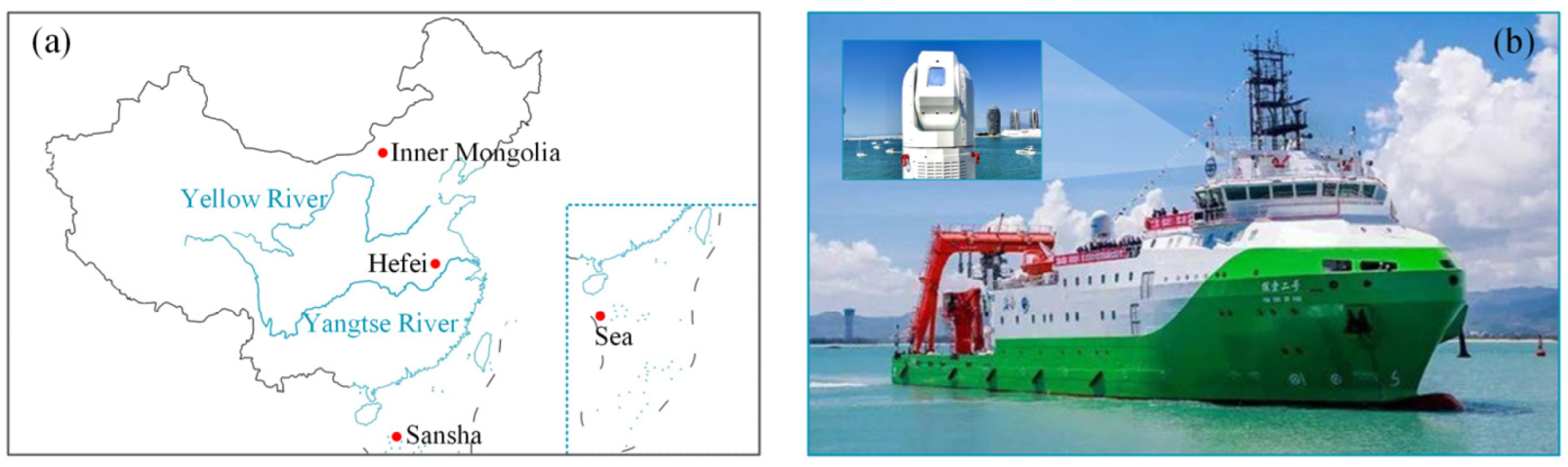
2. Sites, Instruments, and Data

As shown in Figure 1a, the ground-based experiment sites are Xilingole grassland, Inner Mongolia (43°54′N, 115°58′E), University of Science and Technology of China, Hefei (31°50′N, 117°15′E), and Yongxing island, Sansha (16°50′N, 112°20′E). Inner Mongolia and Hefei are inland sites, while Sansha is a marine site. Moreover, the ship-borne experiment site is in the sea (16°25′N, 110°16′E). Figure 1b shows the picture of ship-borne CDWL.

2.1. Coherent Doppler Wind Lidar

An all-fiber micro-pulse CDWL operating at a wavelength of 1548 nm is used [9]. The pulse energy and repetition frequency are 100 µJ and 10 kHz, respectively. The CDWL is operated in a velocity azimuth display (VAD) scanning mode to measure the radial wind velocity along laser beam. It is a conical scanning by a laser beam around the vertical axis with a fixed elevation angle. The elevation angle and azimuth angle resolution are set to 60° and 5°, respectively. The radial range resolution is set to 30 m/60 m in the range of 0–2.5 km/2.5–5.5 km. The period of one scan is about 144 s.

After one scan, the carrier-to-noise ratio (CNR), wind vector, and TKEDR profiles are measured simultaneously. In detail, for every radial measurement, the aerosol backscatter signal is mixed with a local oscillator, obtaining a Doppler signal. The ratio of the Doppler signal power to noise power over the entire spectral bandwidth is the CNR [9]. Then, the wind vector is determined from the sine dependence of radial wind velocity versus azimuth angle [21]. Finally, the TKEDR is estimated by fitting the azimuth structure function of radial wind velocity to a model prediction [22].

2.2. Radiosonde

A radiosonde (GTS1 digital device) is used to measure meteorological parameters, including the relative humidity (RH). The measurement is performed routinely at Zhongsha Islands Meteorological Observation Station, which is close to Sansha. The radiosonde is mounted on a balloon and launched twice a day at 0715 and 1915 LST. The vertical range resolution is about 10 m.

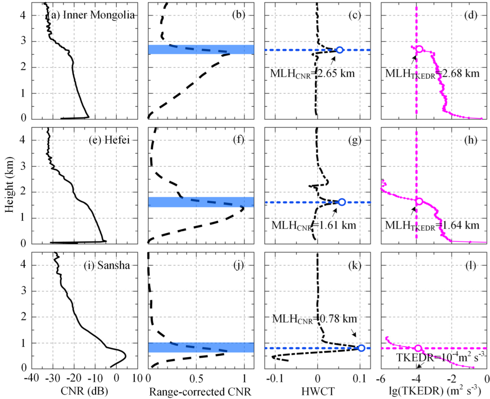
3. Determination of TKEDR Threshold for Retrieving MLH

The MLH can be retrieved from both the aerosol concentration and turbulence intensity. The MLH retrieval results based on aerosol and turbulence are coincident at noon [23]; thus, the MLH retrieval result based on aerosol at noon can be used as a reference to determine the turbulence intensity threshold for retrieving MLH.

The CNR, which is a measure of aerosol backscattered signal, represents aerosol concentration. There is usually a sharp decrease in CNR profile at the ML top because the aerosol concentration in the ML is much higher than that in the free atmosphere. Here, the Haar wavelet covariance transform (HWCT) of CNR is calculated to locate the MLH. The Haar function is defined as [24]:

$$h\left(\frac{z-b}{a}\right)=\{\begin{array}{c}+1, b-a/2\le z\le b\\ -1,b\le z\le b+a/2\\ 0,elsewhere\end{array}$$

(1)

where $z$ is height, $a$ is function dilation, and $b$ is center position. The covariance transform of the function is defined as:

$$W_f\left(a,b\right)=\frac{1}{a}{\int }_{z_b}^{z_t}f\left(z\right)h\left(\frac{z-b}{a}\right)dz$$

(2)

where $f\left(z\right)$ is range-corrected CNR, and $z_b$ and $z_t$ are the bottom height and top height of selected range. For a given dilation $a$, the height of the maximum of local maximums in $W_f\left(a,b\right)$ is the MLH. Moreover, at a well-mixed layer top, there is an entrainment zone where materials are not fully mixed, resulting in a decrease in turbulence intensity. Since the turbulence intensity can be characterized by TKEDR, the MLH is also able to be located via setting an appropriate TKEDR threshold.

Figure 2a–d show the determination process of TKEDR threshold in Inner Mongolia. Figure 2a–c show CNR-related profiles at noon, including CNR measured by CDWL, normalized range-corrected CNR and its HWCT. Figure 2d shows the TKEDR profile measured by CDWL at the same time. To locate the MLH, the CNR is multiplied by the square of range and normalized in a selected range of 0–5 km to obtain the normalized range-corrected CNR at first. Then, its HWCT is calculated according to Equation (2) with a dilation of 250 m. As seen in the blue-shaded area in Figure 2b, there is a sharp decrease in the range-corrected CNR profile. As the range-corrected CNR decreases, its HWCT increases rapidly, resulting in a local maximum. The local maximum height signed by a blue dotted line in Figure 2c is the MLH. Finally, an MLH_CNR of 2.65 km is obtained, which is denoted by a blue circle.

Here, the MLH_CNR is used to determine the value of the TKEDR threshold. Since Inner Mongolia is an inland site, the inland optimum TKEDR threshold of 10⁻⁴ m² s⁻³ is preset and signed by a pink dotted line in Figure 2d. As a result, an MLH_TKEDR of 2.68 km is obtained and denoted by a pink circle. One can see that the MLH_TKEDR agrees well with the MLH_CNR; thus, the threshold preset here is appropriate. Figure 2e–h show the threshold determination at the other inland site (Hefei). The threshold of 10⁻⁴ m² s⁻³ is still appropriate because the obtained MLH_TKEDR of 1.64 km agrees well with the MLH_CNR of 1.61 km. In particular, the threshold determination at the marine site (Sansha) is shown in Figure 2i–l. Since the MLH_CNR is 0.78 km, the MLH_TKEDR is preset as 0.78 km. As a result, the threshold of 10⁻⁴ m² s⁻³ is determined. The results indicate that the inland optimum TKEDR threshold is applicable in retrieving marine MLH.

4. Inland and Marine MLH Detections Using Ground-Based CDWL

The TKEDR threshold method is good at tracing the MLH development and descent processes in the transition periods, including nighttime–daytime and daytime–nighttime. Therefore, it is possible to trace the MLH diurnal evolution. In the ground-based experiments, the MLH diurnal cycles at the inland and marine sites are successfully retrieved. To validate the accuracy of the MLH retrieval result at the marine site, radiosonde-derived MLH is given as a reference.

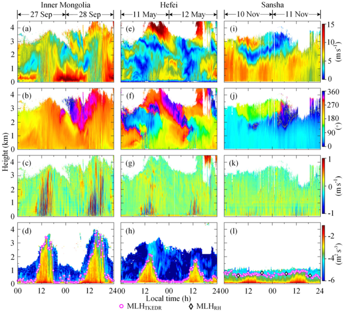
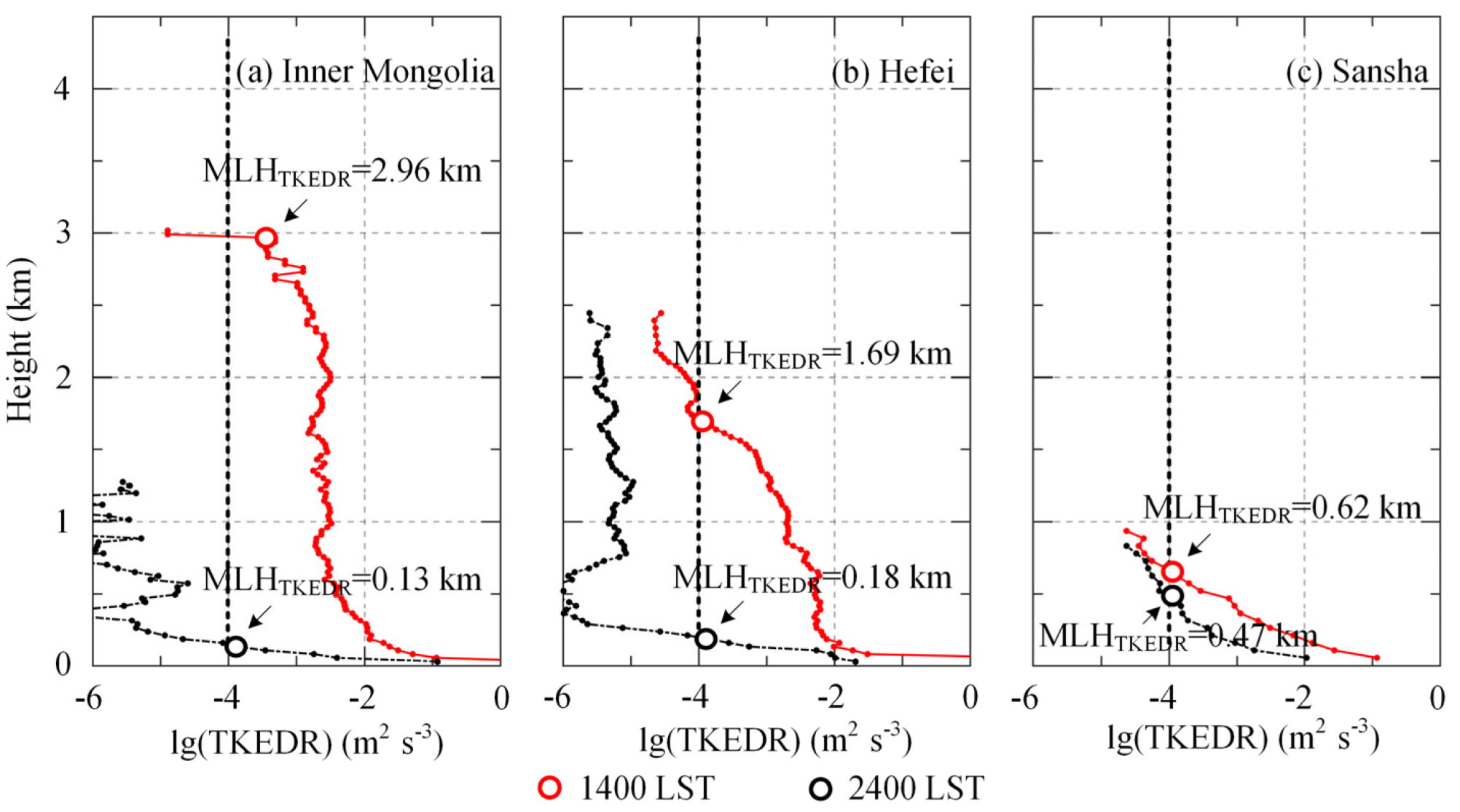
4.1. MLH Diurnal Cycles at the Inland and Marine Sites

Figure 3 shows the two-day ground-based CDWL measurement results and MLH retrieval result. Figure 3a–h show the results at the inland sites (Inner Mongolia and Hefei). The CDWL measurement results include horizontal wind speed, horizontal wind direction, vertical wind speed, and TKEDR. The MLH retrieval result is MLH_TKEDR, which is drawn as pink circle above the TKEDR in Figure 3d,h. There are two significant diurnal cycles in both the TKEDR and MLH. This diurnal cycle is caused by the indirect forcing of solar radiation via the transport process between the ground and atmosphere [1]. Turbulence is one of the important transport processes. After sunrise, the ground surface temperature increases rapidly. The heat is then transmitted to the atmosphere, resulting in an unstable atmosphere stratification. It promotes the generation and development of convective turbulence, and the turbulence intensity reaches its peak at about 1400 LST. The convection is also can be seen in Figure 3c,g with the violent vertical wind. After sunset, the ground surface temperature is gradually lower than the atmosphere temperature due to surface radiative cooling, resulting in a stable stratification with weak turbulence. The MLH diurnal cycle varies with the turbulence diurnal cycle because the MLH is defined by the turbulence intensity. Additionally, the MLH maximum is at about 1400 LST.

The results at the marine site (Sansha) are shown in Figure 3i–l. It is worth noting that compared to Inner Mongolia and Hefei, the convective vertical wind and turbulence are not violent, as shown in Figure 3k,l. Additionally, the diurnal cycle in the MLH is not significant, as shown in Figure 3l. In addition, the MLH retrieval result is distributed mostly over 0.5–1 km. A reasonable explanation is that the sea surface temperature varies slowly due to the large volume and high heat capacity of seawater, thus reducing the impact of solar radiation on the turbulence diurnal cycle. To provide a reference, the MLH_RH retrieved from the RH profile measured by the radiosonde is given [16], which is drawn as a black diamond above the TKEDR in Figure 3l. The MLH_RH shows good agreement with the MLH_TKEDR, validating that the constant TKEDR threshold determined in Section 3 is reliable.

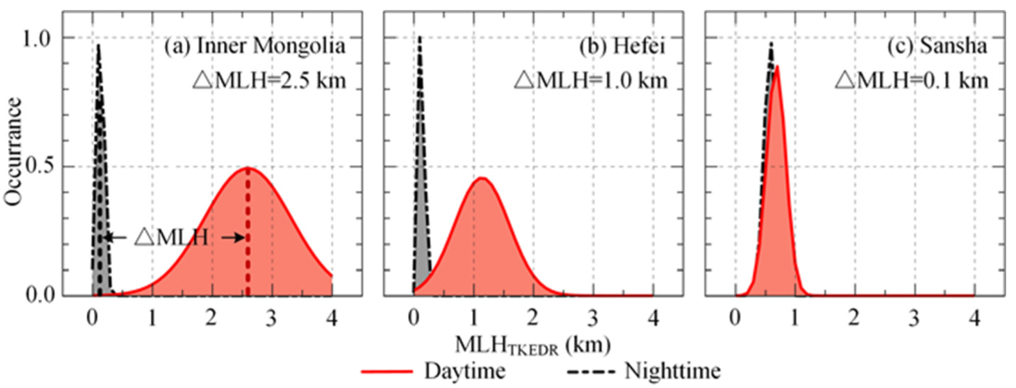
4.2. Comparison of MLH Diurnal Variations over the Inland and Marine Sites

To analyze the MLH diurnal variation, the MLH retrieval results are classified into two conditions of daytime and nighttime [25]. Here, the two conditions are distinguished by the gap between the MLH retrieval results based on aerosol and turbulence. The condition changes from nighttime into daytime when the gap is less than a specified value [11]. The daytime turns into the nighttime again when the gap is larger than the value. A specified value of 500 m is used in Inner Mongolia as the MLH maximum is 3–4 km.

Figure 4 shows a case comparison of the MLH retrieval results at noon and midnight. The TKEDR profiles at noon and midnight on the same day are drawn as a red line and black dash-dotted line, respectively. The red circle and the black circle denote the corresponding MLH retrieval results based on the constant TKEDR threshold. The differences between the MLH retrieval results at noon and midnight in Inner Mongolia, Hefei, and Sansha are 2.83, 1.51, and 0.15 km, respectively. It highlights that the MLH diurnal variation at the marine site (Sansha) is relatively small in this case.

To further compare the MLH diurnal variations over the inland and marine sites, the statistical distributions of MLH retrieval results during ten clear days are performed. As shown in Figure 5, the red line and the black dash-dotted line denote the Gaussian fits of the distributions of MLH retrieval results in daytime and nighttime, respectively. △MLH denotes the difference between the two Gaussian centers. The △MLH in Sansha is 0.1 km, which is much smaller than the △MLH of 2.5 km in Inner Mongolia and the △MLH of 1.0 km in Hefei. The results indicate that the MLH diurnal variation at the marine site (Sansha) is smaller regardless of MLH maximum during this observation.

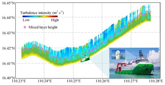
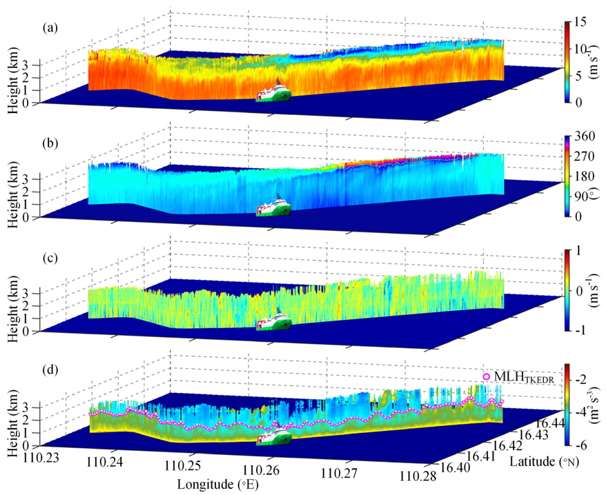
5. Marine MLH Detection Using Ship-Borne CDWL

After validating the reliability of the constant TKEDR threshold, to realize marine MLH detection, the ship-borne experiment was carried out on 05 February 2020 in the west of South China Sea by using a ship-borne CDWL.

The horizontal wind speed, horizontal wind direction, vertical wind speed, TKEDR and its MLH retrieval result along the ship’s route from 16.41°N, 110.23°E to 16.44°N, 110.28°E are measured by the ship-borne CDWL and shown in Figure 6. From Figure 6a, one can see that the wind above the sea surface is uniformly strong due to the less friction at smooth sea underlying surface. From Figure 6b, it can be seen that the wind comes mainly from the northeast because the northeasterly wind is prevalent in South China Sea in winter [26]. The vertical wind and turbulence are shown in Figure 6c,d, respectively. Weak convection can be seen above the sea surface. Based on the constant TKEDR threshold, the marine MLH is successfully detected along the ship’s route in real time, which is drawn as pink circle above the TKEDR in Figure 6d. The MLH detection result is distributed over 1–2 km.

6. Conclusions

Marine MLH detection along the ship’s route is achieved and demonstrated by using a ship-borne CDWL. Before the ship-borne experiment, ground-based experiments are conducted at both inland and marine sites. The optimum TKEDR threshold for retrieving inland and marine MLHs is determined as a constant value of 10⁻⁴ m² s⁻³. The reliability of the constant threshold is then validated at the marine site. During the ground-based observation, the MLH diurnal variation at the marine site is found to be smaller than that at the inland sites in the case of clear day regardless of MLH maximum. In the future, the seasonal comparison of MLH maximums over the inland and marine sites is expected to be performed after long-term observation. Furthermore, using the ship-borne marine MLH detection here, it will be possible to evaluate and improve marine MLH simulation.

References

1. Stull, R.B. An Introduction to Boundary Layer Meteorology; Kluwer Academic Publishers: Dordrecht, The Netherlands, 1988. [Google Scholar]
2. Li, Z.Q.; Zhang, Y.; Shao, J.; Li, B.S.; Hong, J.; Liu, D.; Li, D.H.; Wei, P.; Li, W.; Li, L.; et al. Remote sensing of atmospheric particulate mass of dry PM2.5 near the ground: Method validation using ground-based measurements. Remote Sens. Environ. 2016, 173, 59–68. [Google Scholar] [CrossRef]
3. Zong, L.; Yang, Y.J.; Gao, M.; Wang, H.; Wang, P.; Zhang, H.L.; Wang, L.L.; Ning, G.C.; Liu, C.; Li, Y.B.; et al. Large-scale synoptic drivers of co-occurring summertime ozone and PM 2.5 pollution in eastern China. Atmos. Chem. Phys. 2021, 21, 9105–9124. [Google Scholar] [CrossRef]
4. Luo, T.; Wang, Z.E.; Zhang, D.M.; Chen, B. Marine boundary layer structure as observed by A-train satellites. Atmos. Chem. Phys. 2016, 16, 5891–5903. [Google Scholar] [CrossRef] [Green Version]
5. Sahlée, E.; Smedman, A.S.; Hogstrom, U. Influence of the boundary layer height on the global air–sea surface fluxes. Clim. Dyn. 2009, 33, 33–44. [Google Scholar] [CrossRef]
6. Wildmann, N.; Bodini, N.; Lundquist, J.K.; Bariteau, L.; Wagner, J. Estimation of turbulence dissipation rate from Doppler wind lidars and in situ instrumentation for the Perdigão 2017 campaign. Atmos. Meas. Tech. 2019, 12, 6401–6523. [Google Scholar] [CrossRef] [Green Version]
7. Kohma, M.; Sato, K.; Tomikawa, Y.; Nishimura, K.; Sato, T. Estimate of turbulent energy dissipation rate from the VHF radar and radiosonde observations in the Antarctic. J. Geophys. Res. 2019, 124, 2976–2993. [Google Scholar] [CrossRef] [Green Version]
8. Sathe, A.; Mann, J. A review of turbulence measurements using ground-based wind lidars. Atmos. Meas. Tech. 2013, 6, 3147–3167. [Google Scholar] [CrossRef] [Green Version]
9. Wang, C.; Xia, H.Y.; Shangguan, M.J.; Wu, Y.B.; Wang, L.; Zhao, L.J.; Qiu, J.W.; Zhang, R.J. 1.5 μm polarization coherent lidar incorporating time-division multiplexing. Opt. Express 2017, 25, 20663–20674. [Google Scholar] [CrossRef] [Green Version]
10. Zhang, Y.P.; Wu, Y.B.; Xia, H.Y. Spatial resolution enhancement of coherent Doppler wind lidar using differential correlation pair technique. Opt. Lett. 2021, 46, 5550–5553. [Google Scholar] [CrossRef]
11. Wang, C.; Jia, M.J.; Xia, H.Y.; Wu, Y.B.; Wei, T.W.; Shang, X.; Yang, C.Y.; Xue, X.H.; Dou, X.K. Relationship analysis of PM2.5 and boundary layer height using an aerosol and turbulence detection lidar. Atmos. Meas. Tech. 2019, 12, 3303–3315. [Google Scholar] [CrossRef] [Green Version]
12. Wang, L.; Qiang, W.; Xia, H.Y.; Wei, T.W.; Yuan, J.L.; Jiang, P. Robust Solution for Boundary Layer Height Detections with Coherent Doppler Wind Lidar. Adv. Atmos. Sci. 2021, 38, 1920–1928. [Google Scholar] [CrossRef]
13. Wei, T.W.; Xia, H.Y.; Hu, J.J.; Wang, C.; Shangguan, M.J.; Wang, L.; Jia, M.J.; Dou, X.K. Simultaneous wind and rainfall detection by power spectrum analysis using a VAD scanning coherent Doppler lidar. Opt. Express 2019, 27, 31235–31245. [Google Scholar] [CrossRef] [PubMed]
14. Yuan, J.L.; Xia, H.Y.; Wei, T.W.; Wang, L.; Yue, B.; Wu, Y.B. Identifying cloud, precipitation, windshear, and turbulence by deep analysis of the power spectrum of coherent Doppler wind lidar. Opt. Express 2020, 28, 37406–37418. [Google Scholar] [CrossRef] [PubMed]
15. Jia, M.J.; Yuan, J.L.; Wang, C.; Xia, H.Y.; Wu, Y.B.; Zhao, L.J.; Wei, T.W.; Wu, J.F.; Wang, L.; Gu, S.Y. Long-live High Frequency Gravity Waves in Atmospheric Boundary Layer: Observations and Simulations. Atmos. Chem. Phys. 2019, 19, 15431–15446. [Google Scholar] [CrossRef] [Green Version]
16. Li, H.; Yang, Y.; Hu, X.M.; Huang, Z.W.; Wang, G.Y.; Zhang, B.D.; Zhang, T.J. Evaluation of retrieval methods of daytime convective boundary layer height based on lidar data. J. Geophys. Res. 2017, 122, 4578–4593. [Google Scholar] [CrossRef]
17. Huang, M.; Gao, Z.Q.; Miao, S.G.; Chen, F.; LeMone, M.A.; Li, J.; Hu, F.; Wang, L.L. Estimate of boundary-layer depth over Beijing, China, using Doppler lidar data during SURF-2015. Bound.-Layer Meteorol. 2017, 162, 503–522. [Google Scholar] [CrossRef] [Green Version]
18. Pearson, G.; Davies, F.; Collier, C. Remote sensing of the tropical rain forest boundary layer using pulsed Doppler lidar. Atmos. Chem. Phys. 2010, 10, 5891–5901. [Google Scholar] [CrossRef] [Green Version]
19. Tucker, S.C.; Senff, C.J.; Weickmann, A.M.; Brewer, W.A.; Banta, R.M.; Sandberg, S.P.; Law, D.C.; Hardesty, R.M. Doppler Lidar Estimation of Mixing Height Using Turbulence, Shear, and Aerosol Profiles. J. Atmos. Ocean. Technol. 2009, 26, 673–688. [Google Scholar] [CrossRef]
20. Banakh, V.A.; Smalikho, I.N.; Falits, A.V. Estimation of the height of the turbulent mixing layer from data of Doppler lidar measurements using conical scanning by a probe beam. Atmos. Meas. Tech. 2021, 14, 1511–1524. [Google Scholar] [CrossRef]
21. Banakh, V.A.; Brewer, A.; Pichugina, E.L.; Smalikho, I.N. Measurements of wind velocity and direction with coherent Doppler lidar in conditions of a weak echo signal. Atmos. Ocean. Opt. 2010, 23, 381–388. [Google Scholar] [CrossRef]
22. Banakh, V.A.; Smalikho, I.N. Lidar studies of wind turbulence in the stable atmospheric boundary layer. Remote Sens. 2018, 10, 1219. [Google Scholar] [CrossRef] [Green Version]
23. Dang, R.; Yang, Y.; Hu, X.; Wang, Z.; Zhang, S. A Review of Techniques for Diagnosing the Atmospheric Boundary Layer Height (ABLH) Using Aerosol Lidar Data. Remote Sens. 2019, 11, 1590. [Google Scholar] [CrossRef] [Green Version]
24. Brooks, I.M. Finding boundary layer top: Application of a wavelet covariance transform to lidar backscatter profiles. J. Atmos. Ocean. Technol. 2003, 20, 1092–1105. [Google Scholar] [CrossRef] [Green Version]
25. Coen, M.C.; Praz, C.; Haefele, A.; Ruffieux, D.; Kaufmann, P.; Calpini, B. Determination and climatology of the planetary boundary layer height above the Swiss plateau by in situ and remote sensing measurements as well as by the COSMO-2 model. Atmos. Chem. Phys. 2014, 14, 13205–13221. [Google Scholar] [CrossRef] [Green Version]
26. Wang, G.H.; Su, J.L.; Ding, Y.H.; Chen, D.K. Tropical cyclone genesis over the South China Sea. J. Mar. Syst. 2007, 68, 318–326. [Google Scholar] [CrossRef]
Figure 1. (a) Map of the ground-based experiment sites (Inner Mongolia, Hefei, and Sansha) and the ship-borne experiment site (sea). (b) Picture of ship-borne CDWL.
Remotesensing 14 00745 g001
Figure 2. (a) CNR, (b) normalized range-corrected CNR and its (c) HWCT, (d) lg(TKEDR) profiles at 1202 LST on 27 September 2019 in Inner Mongolia. (eh) is at 1208 LST on 12 May 2019 in Hefei. (il) is at 1209 LST on 10 November 2018 in Sansha. Blue circle and pink circle denote the MLHs retrieved from CNR and TKEDR, respectively.
Remotesensing 14 00745 g002
Figure 3. (a) Horizontal wind speed, (b) horizontal wind direction, (c) vertical wind speed, (d) lg(TKEDR) and its MLH retrieval result measured by ground-based CDWL during 27–28 September 2019 in Inner Mongolia. (eh) is 11–12 May 2019 in Hefei. (il) is 10–11 November 2018 in Sansha. Horizontal wind direction is defined as 0° for northerly wind, rotating clockwise. Negative vertical wind speed denotes rising wind. Pink circle and black diamond denote CDWL-derived MLHTKEDR and radiosonde-derived MLHRH, respectively.
Remotesensing 14 00745 g003
Figure 4. lg(TKEDR) profiles and their MLHTKEDR at 1400 LST (red circle) and 2400 LST (black circle) on (a) 27 September 2019 in Inner Mongolia, (b) 11 May 2019 in Hefei, and (c) 10 November 2018 in Sansha.
Remotesensing 14 00745 g004
Figure 5. Statistical distributions of MLHTKEDR in daytime (red line) and nighttime (dash-dotted line) during (a) 21–30 September 2019 in Inner Mongolia, (b) 09–18 May 2019 in Hefei, and (c) 05–14 November 2018 in Sansha.
Remotesensing 14 00745 g005
Figure 6. (a) Horizontal wind speed, (b) horizontal wind direction, (c) vertical wind speed, (d) lg(TKEDR) and its MLH retrieval result measured by ship-borne CDWL along the ship’s route in the Sea. Pink circle denotes MLHTKEDR.
Remotesensing 14 00745 g006
Publisher’s Note: MDPI stays neutral with regard to jurisdictional claims in published maps and institutional affiliations.