Multiscale Feature Fusion Network Incorporating 3D Self-Attention for Hyperspectral Image Classification

Abstract

In recent years, the deep learning-based hyperspectral image (HSI) classification method has achieved great success, and the convolutional neural network (CNN) method has achieved good classification performance in the HSI classification task. However, the convolutional operation only works with local neighborhoods, and is effective in extracting local features. It is difficult to capture interactive features over long distances, which affects the accuracy of classification to some extent. At the same time, the data from HSI have the characteristics of three-dimensionality, redundancy, and noise. To solve these problems, we propose a 3D self-attention multiscale feature fusion network (3DSA-MFN) that integrates 3D multi-head self-attention. 3DSA-MFN first uses different sized convolution kernels to extract multiscale features, samples the different granularities of the feature map, and effectively fuses the spatial and spectral features of the feature map. Then, we propose an improved 3D multi-head self-attention mechanism that provides local feature details for the self-attention branch, and fully exploits the context of the input matrix. To verify the performance of the proposed method, we compare it with six current methods on three public datasets. The experimental results show that the proposed 3DSA-MFN achieves competitive classification and highlights the HSI classification task.

1. Introduction

A hyperspectral image is a combination of imaging and spectroscopy to obtain high-dimensional spatial and spectral information simultaneously. Since ground features have different characteristics in different dimensions, their dense spectral dimensions provide good conditions for the accurate classification of ground features. Therefore, hyperspectral images have a wide range of applications in agricultural production, environmental and climate detection, urban development, and military security [1,2,3,4,5,6,7,8]. In the early days, conventional machine learning classification methods were used to classify hyperspectral images [9,10,11,12,13,14,15,16], such as the K-nearest neighbor algorithm (KNN) [9], support vector machine (SVM) [10,11], and random forest (RF) [12], which are unable to automatically learn deep features and rely on prior expert knowledge, making effective feature extraction difficult for datasets with high-order nonlinear distributions.

In recent years, HSI classification methods based on deep learning have become increasingly popular. Because deep learning can extract deep abstract features effectively, it has gradually replaced the previous classification model with manually created features. Deep learning uses an end-to-end learning strategy which greatly improves the performance of HSI classification. Chen et al. [17] proposed a deep belief network (DBN), that combines spectrum-space finite elements and classification to improve the accuracy of HSI classification. Zhao et al. [18] constructed a spatial-spectral joint feature set and used a stacked sparse autoencoder (SAE) to extract image features. Deng et al. [19] proposed a unified deep network using a hierarchical stacked sparse autoencoder (SSAE) network to extract the deep joint spectral features. Since these methods compress the spatial dimension into a vector, they ignore the spatial correlation and local consistency of the HSI, which often results in the loss of spatial information.

Subsequently, two-dimensional convolutional neural networks have been introduced to the HSI task. Cao et al. [20] integrated spectral and spatial information into a unified Bayesian framework and used convolutional neural networks to learn the posterior distribution. Hao et al. [21] used a three-layer Super Resolution convolutional neural network to create high-resolution images and then constructed an unsupervised triple convolutional network (TCNN). Pan et al. [22] proposed an end-to-end segmentation method that can directly label each pixel. Li et al. [23] used two two-dimensional convolutional neural networks to extract spectral, local spatial, and global spatial features simultaneously. To adaptively learn the fusion weights of spectral spatial features from two parallel streams, a fusion scheme with hierarchic regularization and smooth normalization fusion was proposed. Yang et al. [24] proposed an HSI classification model using spatial background and spectral correlation. These methods improve the classification performance of HSI to a certain extent; however, since the two-dimensional convolution kernel cannot use the context between the spectral cores, spectral spatial information is easily lost.

To solve this problem, some studies introduced the attention mechanism into the HSI classification task, and chose to extract the spectral and spatial features separately. Sun et al. [25] proposed a spectral-spatial attention network (SSAN), used to extract the information from the HSI. In this approach, characteristic spectral-spatial features are captured in the attention area of the cube while the influence of interfering pixels is suppressed. Zhu et al. [26] proposed a dual-attention boost residual frequency-doubling network. In feature extraction, the high -and low-frequency components are convolved separately, and dual self-attention is used to output the feature map. It is improved to obtain a refined feature map. Zhu et al. [27] proposed an end-to-end residual spectrum and spatial attention network, that directly processed the original three-dimensional data, and used dual attention modules for adaptive feature refinement for spectral spatial feature learning. Li et al. [28] designed a spatial-spectral attention block (S2A) to simultaneously capture the long-term interdependence of spatial and spectral data through similarity assessment. Qing et al. [29] proposed a multiscale residual network model with an attention mechanism (MSRN). The model uses an improved residual network and a spatial–spectral attention module to extract hyperspectral image information from different scales multiple times and fully integrate and extract the spatial spectral features of the image. In addition, some studies have used 3-dimensional convolutional nerves, which can better utilize the contextual information of the bands between spectra for HSI classification [30,31,32,33,34,35]. Lu et al. [30] proposed a new multi-scale spatial spectrum residual network (CSMS-SSRN) based on three-dimensional channels and spatial attention, which continuously learns the spectrum and space from the respective residual blocks through different three-dimensional convolution kernels features. Tang et al. [32] proposed a three-dimensional convolutional frequency multiplication space-spectral attention network (3DOC-SSAN) that can simultaneously mine spatial information from both high and low frequencies and simultaneously acquire spectral information. Farooque et al. [33] proposed a residual network (SSCRN) based on end-to-end spectral space three-dimensional ConvLSTM-CNN, that combines three-dimensional ConvLSTM and three-dimensional CNN to process spectral and spatial information, respectively. Lu et al. [34] proposed a three-dimensional cascaded spectrum-spatial element attention network (3D-CSSEAN), in which two attention modules can focus on the main spectral features and meaningful spatial features. Yin et al. [35] used a three-dimensional convolutional neural network and bidirectional long short-term memory network (Bi-LSTM) based on band grouping for HSI classification.

Although the convolution operation has the advantages of spatial locality and shared weights, it has also achieved great advantages in the HSI classification task. However, it is difficult to model long-distance dependencies using the convolutional neural network, and is difficult to capture the global feature representation. Since multi-head self-attention can capture long-distance interactions well, the transformer module with multi-head self-attention has been applied to the HSI classification task in many works. He et al. [36] proposed a HSI-BERT model with a global receptive domain. This model supports dynamic input regions without considering the spatial distance between pixels, and directly captures the global dependencies between pixels. Qing et al. [37] proposed an end-to-end transformer model called SAT-Net, which uses a spectral attention and self-attention mechanism to extract the spectral and spatial features of HSI and capture the long-distance continuous spectrum relation. He et al. [38] explored the spatial transformation network (STN), and Zhong et al. [39] proposed a spectrum-spatial transformer network (SSTN) consisting of a spatial attention module and spectrum correlation module. Gao et al. [40] combined the transformer and CNN and used the stage model to extract coarse -and fine-grained feature representations at different scales of implication.

Inspired by the above methods, to fully exploit the joint spectral-spatial information essential for the HSI classification, we propose a multiscale feature fusion network that incorporates 3D self-attention for HSI classification tasks. The network first uses convolution kernels of different sizes for multiscale feature extraction and adds the feature results extracted from different branches to perform effective feature fusion. Then, the proposed 3DCOV_attention block is used multiple times to improve the feature extraction of the obtained feature map, while modeling the global dependency relationship, performing comprehensive feature extraction from local to global, and improving the local receptive field while capturing long-distance interactions. At the end, the output feature map is flattened and converted into a one-dimensional vector, successively passed through several fully connected layers, to finally output the classification result.

The main contributions of this work are as follows:

• We propose a multiscale feature fusion module to sample the different granularities of the feature map and effectively fuse the spatial and spectral features of the feature map.
• We propose an improved 3D multi-head self-attention module that provides local feature details for self-attention branches while fully utilizing the context of the input matrix.
• We propose a 3DCOV_attention block which combines convolutional mapping that extracts local features, with self-attention feature mapping that can be globally dependent, and improving the feature extraction capabilities of the entire network.
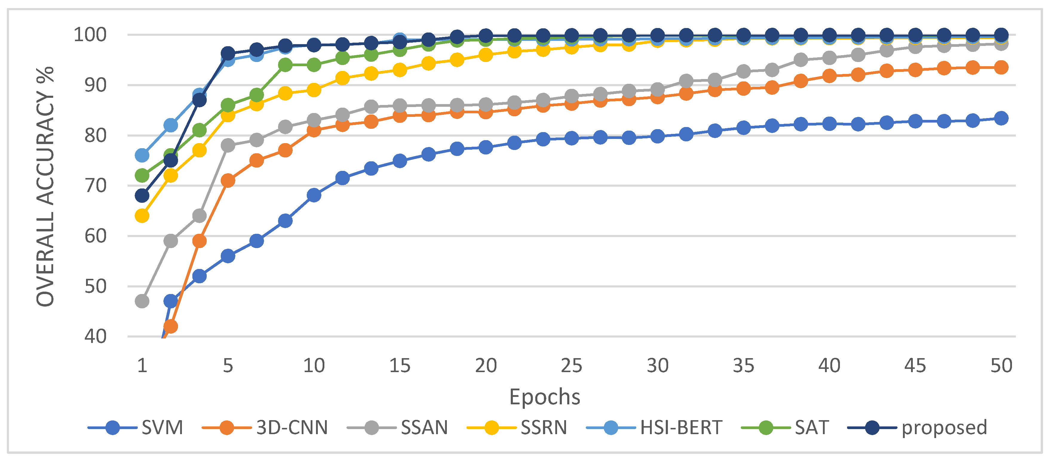
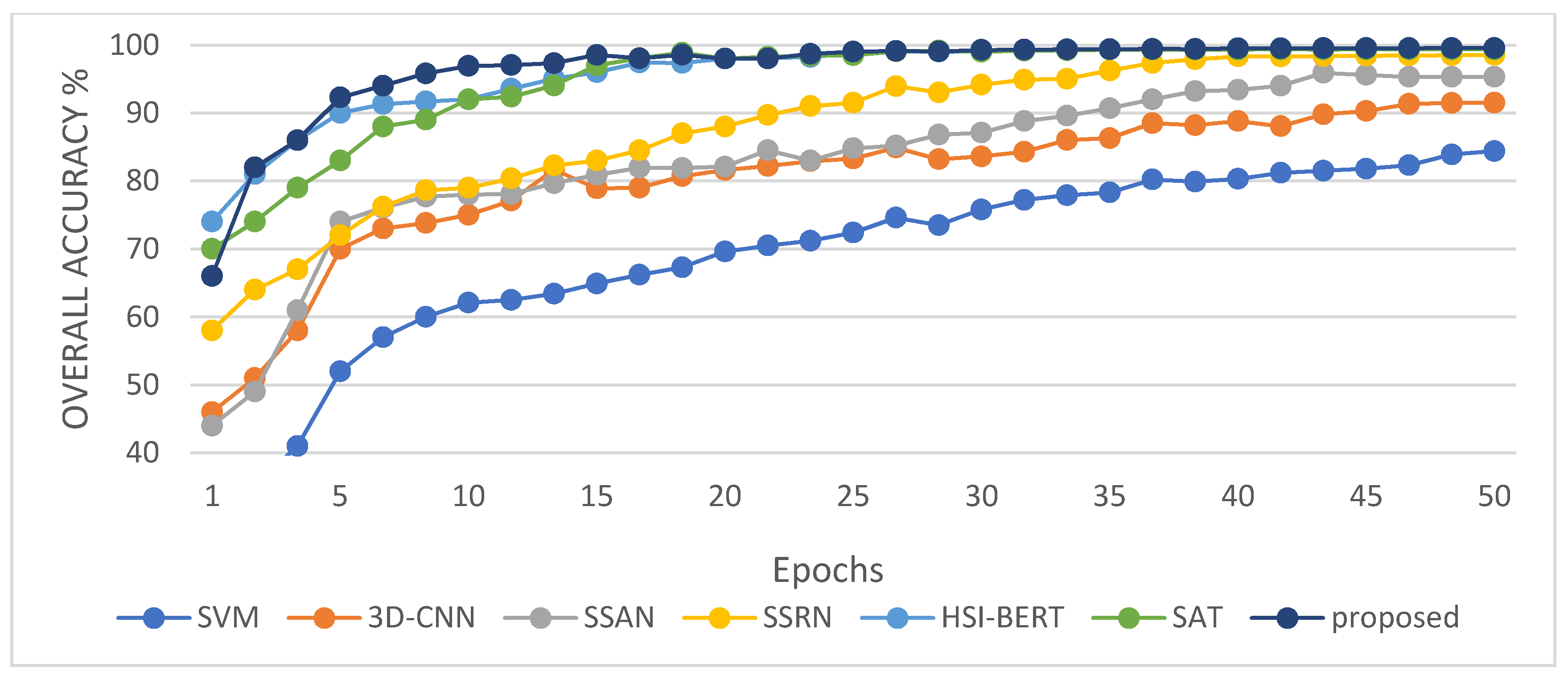
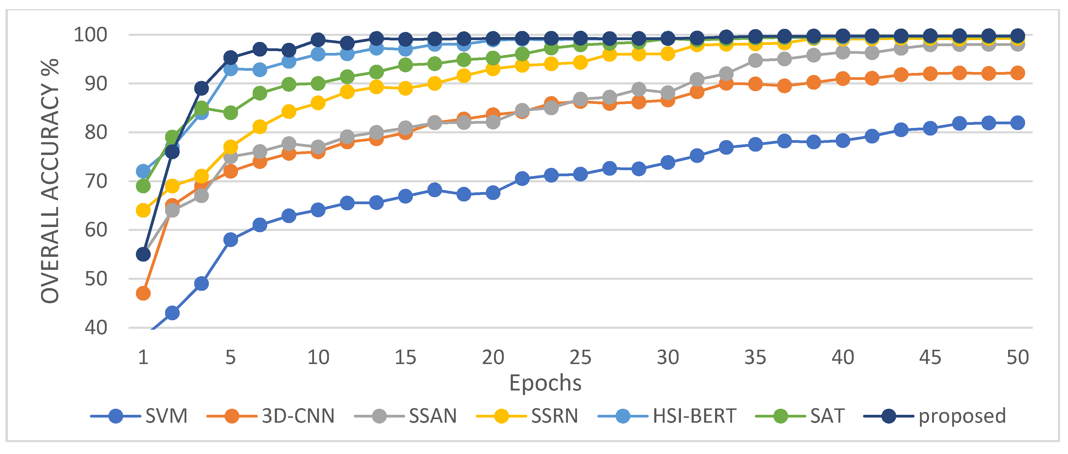
• Experimental evaluation of the HSI classification against six current methods highlights the effectiveness of the proposed 3DSA-MFN model.

The remainder of this study is organized as follows. In the second section the proposed 3DSA-MFN, multi-scale feature fusion module, improved 3D self-attention, 3DCOV_attention, and other modules, and the corresponding loss function are presented in detail. The third section presents the ablation and comparative experiments. The fourth section summarizes this article.

2. Materials and Methods

In this section, we first introduce the proposed 3DSA-MFN network, then explain the multiscale feature fusion module and the improved 3D multi-head self-attention module, and then present the 3DCOV_attention module in detail and explain the formula derivation. Finally, the loss function and optimization method of the network framework are presented.

2.1. Overview of the Proposed Model

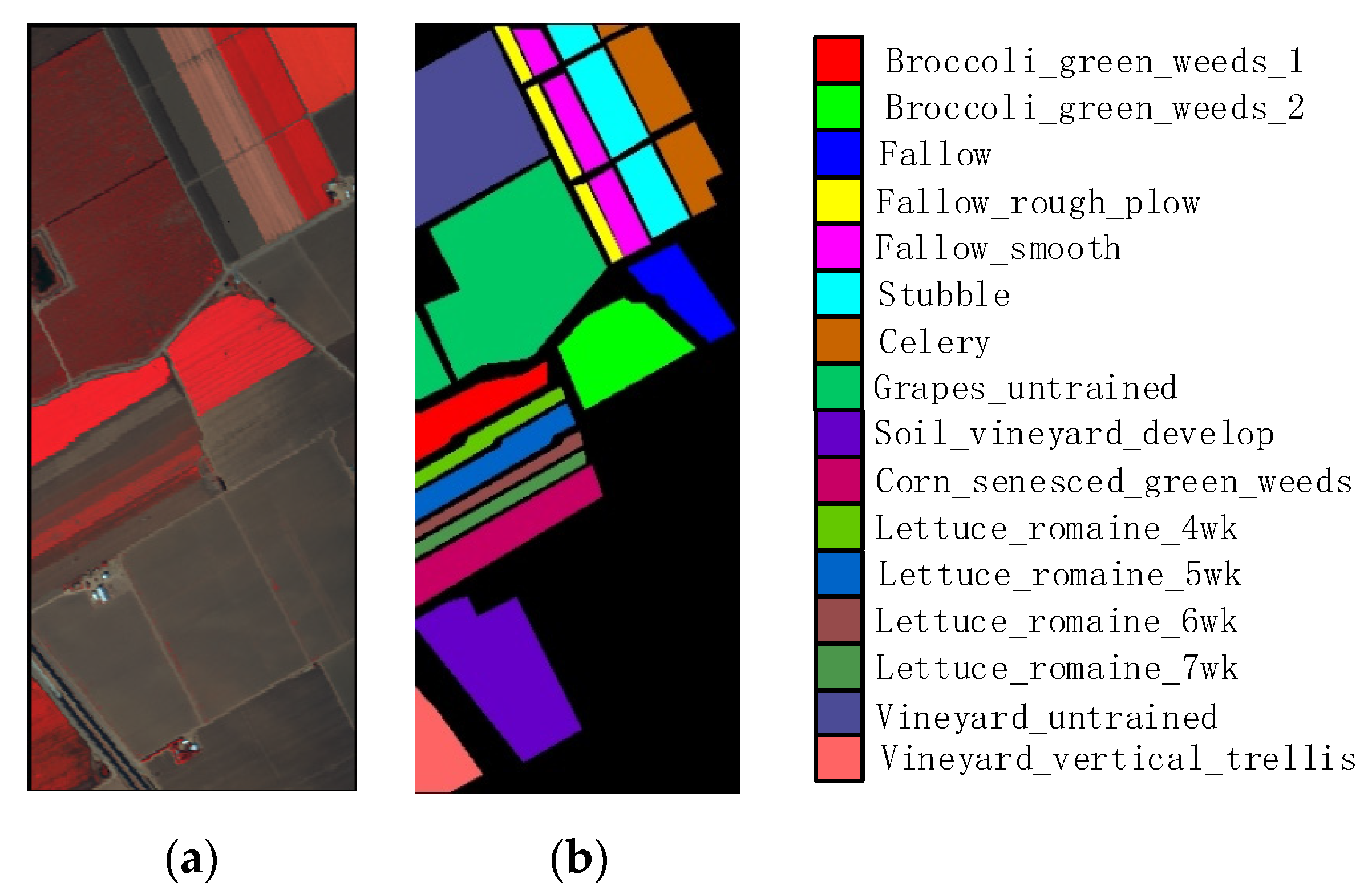
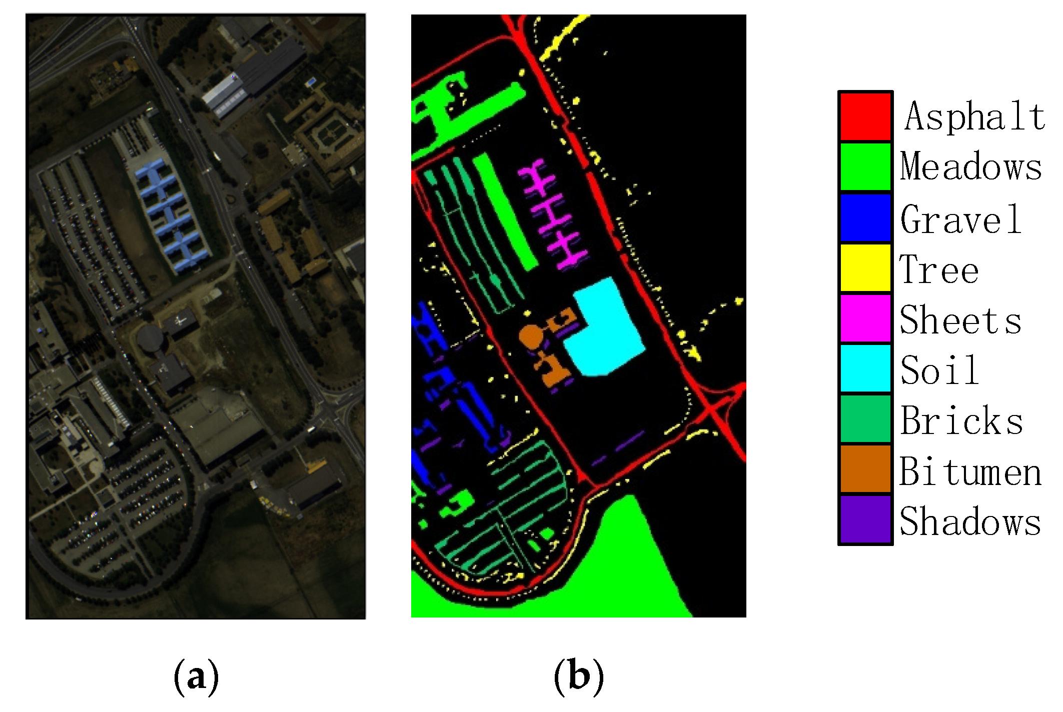
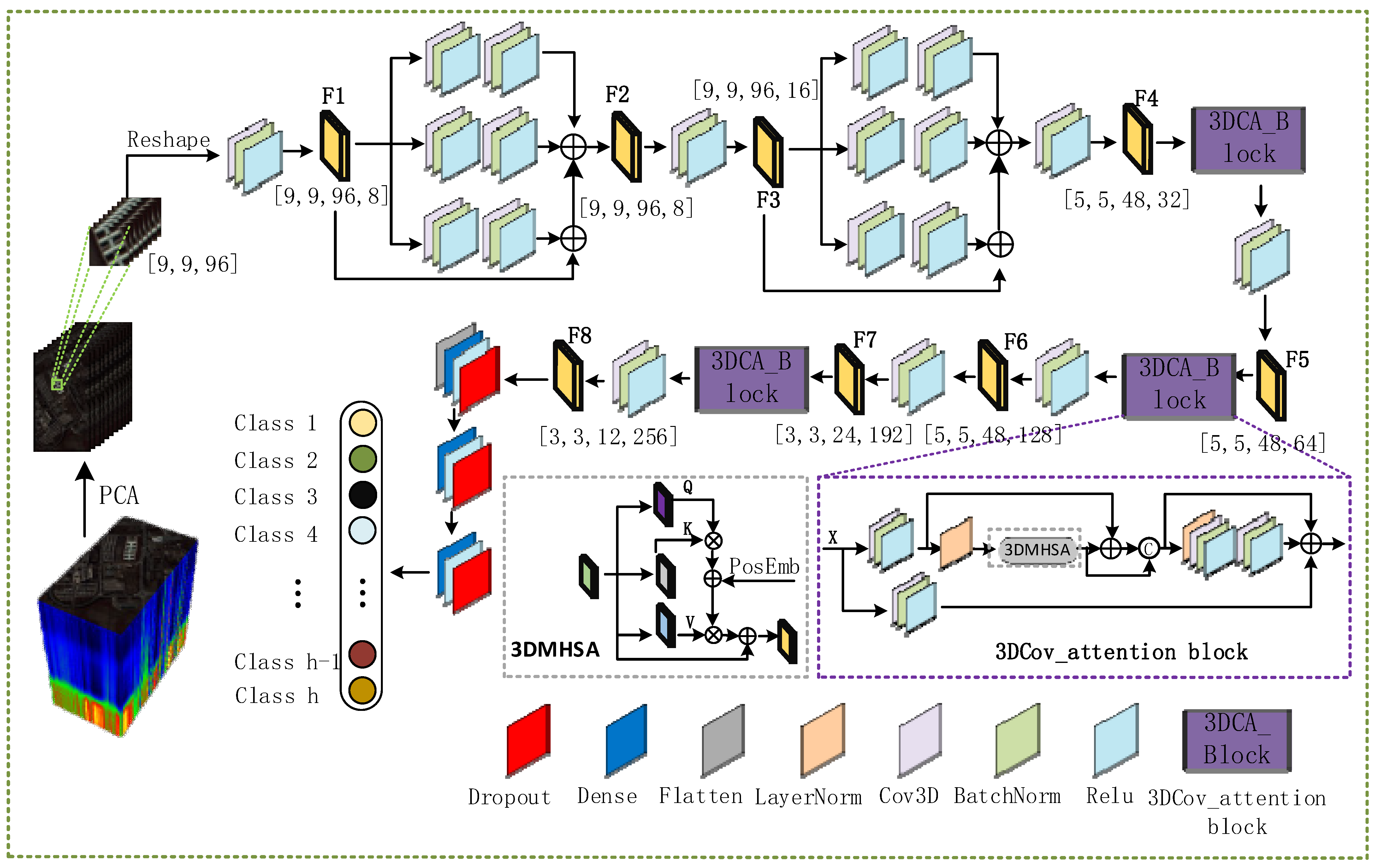
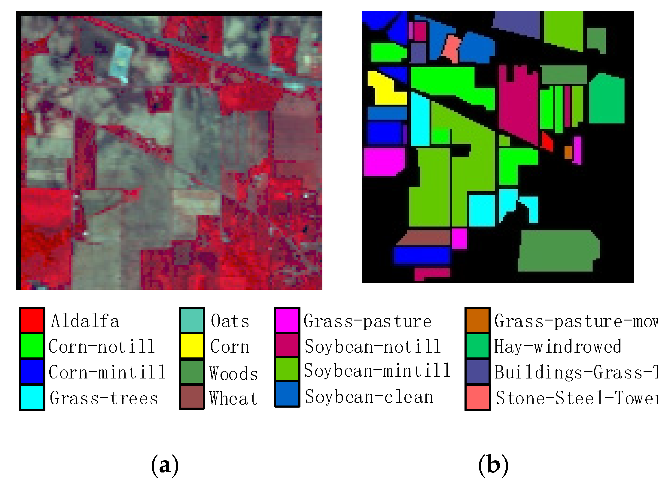
Since hyperspectral data is three-dimensional, and the number of spectra is usually tens or hundreds, extremely high resolution can better determine the characteristics of ground objects. However, the collection of extremely high-resolution images often contains a large amount of noise, and redundant data will affect the results of hyperspectral classification. We first applied the Principal Component Analysis (PCA) algorithm to the original hyperspectral data. Following a linear transformation strategy, the noise and redundant bands were removed while reducing the dimensionality of the data. Then, a 9 × 9 size window was used to process the reduced data. Data of the corresponding size were obtained as a sample, and the sample was randomly divided into a training set, a test set, and a verification set. We first passed the processed data samples through two multiscale feature fusion modules to extract the features of the hyperspectral image while reducing the shape of the feature map and increasing the number of feature maps. Then, we continuously passed the output feature map through three 3DCOV_attention modules to further extract the hyperspectral image features while modeling the global dependencies. At the same time, we used the 3D convolution from step 2 in different 3DCOV_attention modules to change the feature map shape. Finally, the output feature map was passed through multiple fully connected layers to output the final classification result. These parts are presented in detail in later sections. The overall process is shown in Figure 1.

Specifically, after processing the original data by the PCA algorithm and a 9 × 9 window, multiple data with a size of {9, 9, 96} were obtained. We first expand the dimensions to fit the data format to the 3D volume-product neural network; the size of the expanded feature map is {9, 9, 96, 1}. The expanded feature map is first passed through a CBR block with a convolution kernel of 3 × 3 × 3, a step size of 1 × 1 × 1, and a filter of 8 (CBR block refers to 3D convolutional neural network, BatchNorm, and ReLU activation function modules are executed sequentially), and the feature map F1 of size {9, 9, 96, 8}, then input F1 into a multi-scale feature fusion module, and add the three feature maps and F1 to obtain the feature map F2 of size {9, 9, 96, 8}. Pass F2 through a CBR block with a convolution kernel of 3 × 3 × 3, a step size of 1 × 1 × 1, and a filter of 16 to further increase the number of feature maps and obtain Feature map F3 of size {9, 9, 96, 16}. Similar to the conversion of feature map F1 to feature map F2, feature map F3 obtains a feature map of the same size ({9, 9, 96, 16}) after the multi-scale feature fusion module and passes it through a convolution kernel into 1 × 1 × 1, a step size of 2 × 2 × 2, and a CBR block with a filter of 32 to obtain a feature map F4 with a size of {5, 5, 48, 32}. After F4 passes through a 3DCOV_attention module that does not change the shape of the feature map, it passes through a CBR block with a convolution kernel of 1 × 1 × 1, a step size of 1 × 1 × 1, and a filter of 64 to obtain a size of {5, 5, 48, 64}. The feature map F5 to feature map F6 is the same as the operation of feature map F4 to feature map F5. From F5, we obtain a feature map F6 of size {5, 5, 48, 128}. F6 first passes through a CBR block with a convolution kernel of 1 × 1 × 1, step size of 2 × 2 × 2, and filter of 192 to obtain the feature map F7({5, 5, 48, 64}). F7 goes through after the 3DCOV_attention module, passes a CBR block with a convolution kernel of 1 × 1 × 1, a step size of 1 × 1 × 2, and a filter of 256 to obtain the feature map F8({3, 3, 12, 256}). Finally, after the flattening operation, F8 is converted into a one-dimensional vector, and then passed through the fully connected module of size 256 and 128 (dropout is 0.5). Finally, the classification result is output.

2.2. Multi-Scale Feature Fusion Module

Many studies have shown that the feature information extracted in different scales is different, and the feature extraction in a single scale often misses some feature information. Therefore, many methods use multiscale feature extraction to improve the feature extraction capability of the network. Szegedy et al. [41] proposed a module called Inception, which contains four parallel branch structures: 1 × 1 convolution, 3 × 3 convolution, 5 × 5 convolution, and 3 × 3 maximum pooling. This module performs feature extraction and pooling at different scales to obtain multiple scales of information. Finally, the features are superimposed and output, and the sparse matrix is clustered into denser submatrices to improve the computational performance. Chen et al. [42] proposed a network called Deeplab V3, which added a multi-scale feature extraction module ASPP [42] and parallel sampling of the given input with different sampling rates of the whole convolution at the end of its feature extraction network which is equivalent in the context of multiple scale image acquisition. Zhao et al. [43] proposed a pyramid pool module and pyramid scene analysis network. The acquired feature layer was divided into grids of different sizes, and each grid was internally averaged. The aggregation of contextual information in different areas is realized, which improves the ability to obtain global information. Chen et al. [44] created a multibranch network and frequently merged branch features of different scales to obtain multiscale features. 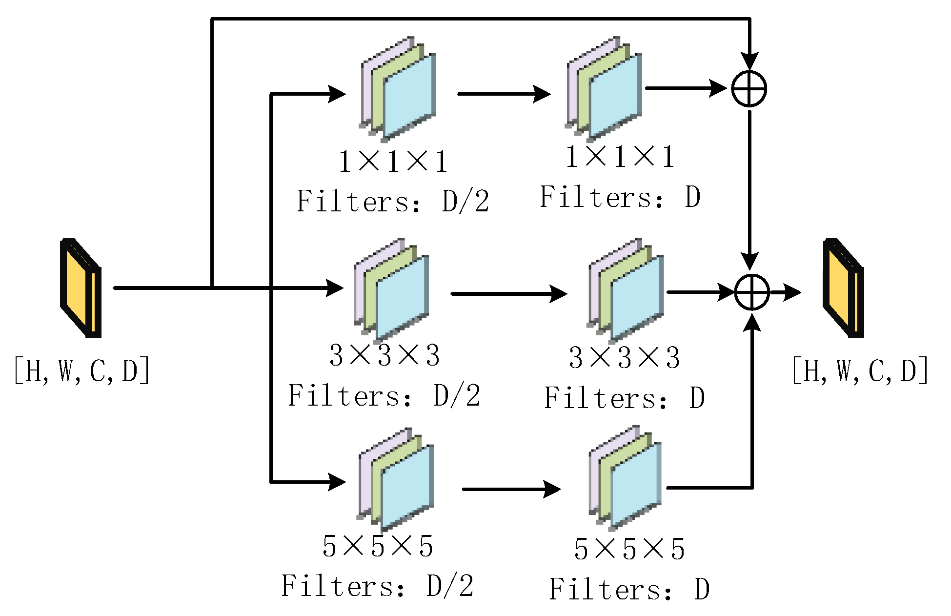Inspired by the above methods, we propose a multiscale feature-fusion module, as shown in Figure 2. We use convolution kernels of different sizes for multiscale feature extraction on the input feature map, and finally add the feature results extracted from different branches to the output, sample the different granularities of the feature map, and fuse the spatial and spectral features of the feature map effectively.

When we input the feature map of size {H, W, C, D}, the feature map is first sent to the CBR of the convolution kernel size of 1 × 1 × 1, 3 × 3 × 3, and 5 × 5 × 5 in the module (execute 3D convolution, BatchNorm, and Relu activation functions in sequence), the filters are D/2, and the feature map of size {H, W, C, D/2} is obtained. The obtained feature maps were sent to the CBR modules with convolution kernel sizes of 1 × 1 × 1, 3 × 3 × 3, and 5 × 5 × 5, respectively, and the filters were D. At this time, three feature maps of sizes {H, W, C, D} were obtained, and finally, the three results were added to the input to obtain the final output feature map.

2.3. Improved 3D Multi-Headed Self-Attention

The attention mechanism originally refers to the fact that people pay more attention to interesting information while ignoring less important information. Bahdanauet et al. [45] first applied the attention mechanism to the field of natural language processing, and subsequently self-attention has been used in many studies in the field of machine translation and natural language processing [46,47,48,49]. Attention has also been applied in the field of computer vision. Dosovitskiy et al. [50] cut the original image into patches of different sizes and then sent the cut region into a transformer block consisting of multi-headed self-attention and other structures to extract features for image classification. Touvron et al. [51] added a feedforward network (FFN) on top of a multi-head self-attention layer and introduced a specific teacher-student strategy for image classification tasks. For the target detection task, Zhu et al. [52] proposed a variable attention module, and Carion et al. [53] proposed a new design for object detection systems based on transformers and bipartite matching loss for direct set prediction. In the segmentation task, Zheng et al. [54] and others employed a pure transformer module with multi-headed self-attention as a component and established a global context.

However, these designs on the one hand, project the image patch onto the vector, resulting in a loss of local detail [55]. In a CNN, the convolution kernel slides on overlapping feature maps, which provides the opportunity to retain detailed local features. Therefore, the CNN branch can continuously provide local feature details to the self-attention branch. On the other hand, the existing self-attention directly obtains the attention matrix of Q and K at each spatial position (see the next paragraph for a detailed definition). Ignoring the contextual relationship between adjacent K matrices [56], after using the CNN operation, the local spatial context can be further captured and the semantic ambiguity in the attention mechanism can be reduced [57]. Therefore, in this study, we used a three-dimensional convolutional neural network operation with a convolution kernel of size 1 × 1 × 1 to replace the linear projection operation in the above method. The convolution kernel has overlapping sliding in the input feature map, and retains the detailed local features of the feature map, but on the other hand, makes full use of the context information between the input matrix K.

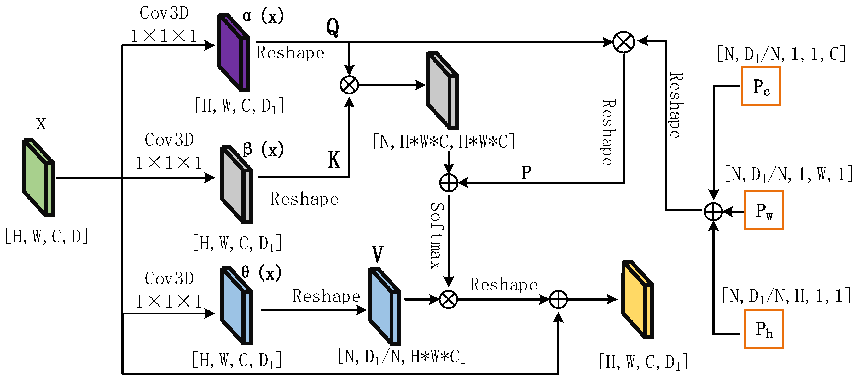
Specifically, we define the input feature map $\mathrm{x}\mathsf{ϵ}{\mathbb{R}}^{\mathrm{H}\times \mathrm{W}\times \mathrm{C}\times \mathrm{D}}$, where H and W represent the length and width of the feature map, respectively, C represents the number of spectra of the feature map (number of channels), and D represents the feature map quantity. We first map the input feature map to three feature spaces a $\left(\mathrm{x}\right)\mathsf{ϵ}{\mathbb{R}}^{\mathrm{H}\times \mathrm{W}\times \mathrm{C}\times \mathrm{D}1}$, $\mathsf{\beta }\left(\mathrm{x}\right)\mathsf{ϵ}{\mathbb{R}}^{\mathrm{H}\times \mathrm{W}\times \mathrm{C}\times \mathrm{D}1}$ and $\theta \left(\mathrm{x}\right)\mathsf{ϵ}{\mathbb{R}}^{\mathrm{H}\times \mathrm{W}\times \mathrm{C}\times \mathrm{D}1}$, and then reshape the feature maps in the a(x), β(x) and θ(x) spaces to obtain three matrices Q, K and V, respectively, as shown in Equation (1):

$$\{\begin{array}{c}\mathrm{Q}=\mathrm{Reshape}\left(\mathrm{Cov3D}\left(\mathrm{x}\right)\right)\\ \mathrm{K}=\mathrm{Reshape}\left(\mathrm{Cov3D}\left(\mathrm{x}\right)\right)\\ \mathrm{V}=\mathrm{Reshape}\left(\mathrm{Cov3D}\left(\mathrm{x}\right)\right)\end{array}$$

(1)

Cov3D represents a three-dimensional convolutional layer with a convolution kernel size of 1 × 1 × 1, and $\mathrm{Reshape}(·)$ represents a reshaping operation on the shape of the obtained feature map.

Then, we perform the inner product operation on Q and ${\mathrm{K}}^{\mathrm{T}}$, match sequence Q with K, obtain the attention map, and obtain the attention score. The attention score of each pixel represents the relationship between each pixel and the target feature. The attention is not sensitive to the order of the input vector. Like [58,59], we add a relative position bias P here. Then, the attention map is standardized to the attention weight using the softmax function. Subsequently, we aggregate all the values of V, use the attention weight to calculate the output of the final attention matrix, and perform the Reshape operation to the final output, as shown in Equation (2).

$$3\mathrm{DMHSA}\left(\mathrm{Q},\mathrm{K},\mathrm{V}\right)=\mathrm{Reshape}\left(\mathrm{Softmax}\left(\mathrm{Q}·{\mathrm{K}}^{\mathrm{T}}+\mathrm{P}\right)\mathrm{V}\right)$$

(2)

As shown in Figure 3, P is obtained by adding three random position codes, where the H, W, C, and Q matrices are the same. After performing the reshape operation, the position codes are multiplied by the Q matrix to obtain the position code P.

Given the feature map x of the shape {H, W, C, D}, we first pass through three convolution kernels of size 1 × 1 × 1 and a three-dimensional convolution of step size of 1 × 1 × 1 to obtain three A feature maps with a shape of {H, W, C, D}. After performing the reshape operation on them, we obtain three matrices Q, K, and V with sizes {N, D/N, H*W*C}, where the context information and local feature details are preserved, and N is the number of heads. Then, the matrices Q and K are multiplied to obtain an attention matrix of size {N, H*W*C, H*W*C }. To confirm the position information between images, we introduce position coding information here. Initialize three matrices with sizes {N, D/N, H, 1,1}, {N, D/N, 1, W,1}, {N, D/N, 1, 1,C}. It should be noted that H, W, and C here are the H, W, and C of Q matrix. As shown in Figure 3, we first add the three position matrices to obtain a matrix of size {N, D/N, H, W, C}, perform the reshaping operation, and multiply it by the Q matrix to obtain the final position coding matrix P. The position coding matrix P is added to the attention matrix, and multiplied by matrix V after the Softmax activation function to output a matrix of shape {N, D/N, H*W*C }. After performing the reshaping operation, the output is a feature map of size {H, W, C, D}.

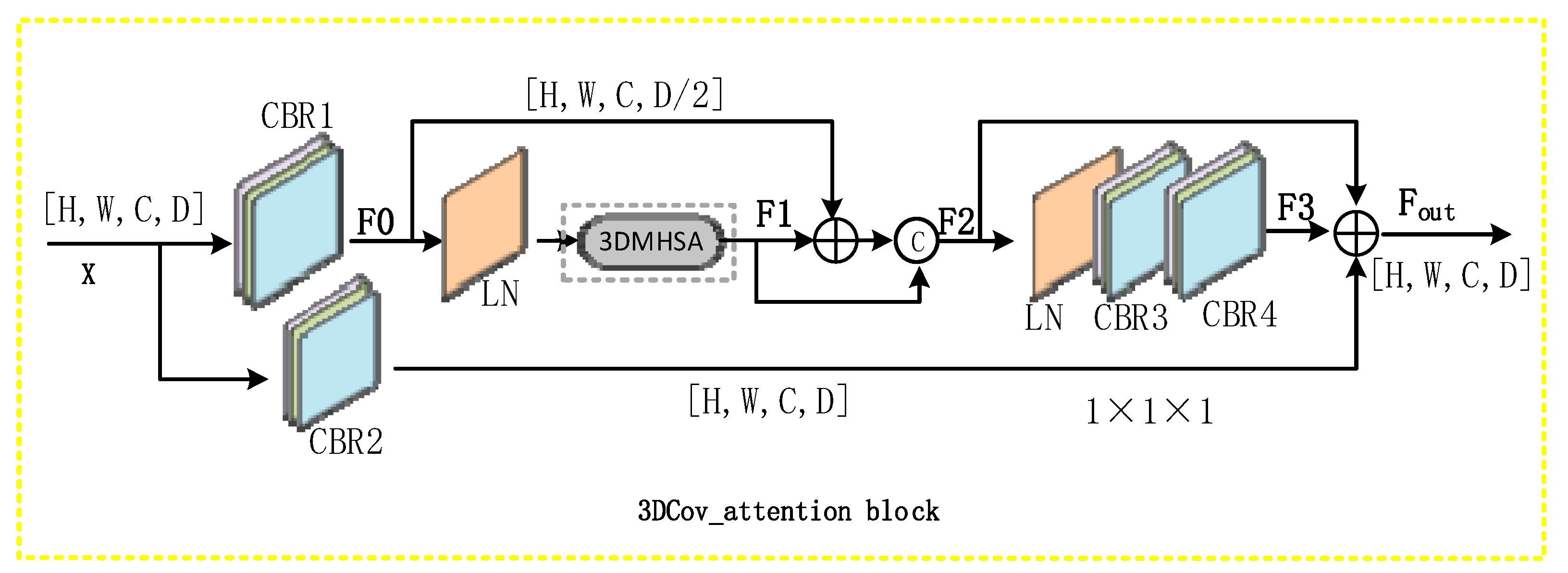
2.4. DCOV_Attention Block

In convolutional neural networks (CNN), the convolution operation is based on discrete convolution operators. It has the properties of spatial locality and variance, such as translation and shared weights. It is now widely used in computer vision tasks [60,61,62,63]. However, the convolution operation only works in the local neighborhood and is effective in extracting local features. In turn, the limited receptive domain hinders the modeling of global dependencies, and it is difficult to capture the global representation, resulting in the loss of global features. However, since self-attention can capture interactions over long distances, it is widely used in computer vision. Currently, many methods combine self-attention and convolution operations [64,65,66,67,68,69,70]. Srinivas et al. [64] used global self-attention instead of spatial convolution in the last three bottleneck blocks of the ResNet. Graham et al. [67] proposed a CNN and transformer hybrid neural network. At the front end of the proposed method, a convolutional neural network was used to first extract image features, and then a self-attention module was used to produce global dependencies. Wang et al. [70] proposed a pyramid vision transformer which could improve the performance of many downstream tasks. Inspired by the above methods, we applied it to a three-dimensional convolutional neural network and used a 3D self-attention mechanism to improve the convolution. We created a 3DCOV_attention block, that combines the convolution map that extracts local features with the self-attention feature map which can establish a global dependency to enhance the local receptive field while capturing interactions over a long distance. As shown in Figure 4, the entire module consists of three-dimensional convolution, BatchNorm, activation function (Relu), LayerNorm, concatenate, 3DMHSA, and other components, as shown in Equation (3).

$$\{\begin{array}{c}\mathrm{F}0=\mathrm{CB}{\mathrm{R}}_1\left(\mathrm{x}\right)\\ \mathrm{F}1=3\mathrm{DMHSA}\left(\mathrm{LN}\left(\mathrm{F}0\right)\right)\\ \mathrm{F}2=\mathrm{Con}\left(\mathrm{F}1,\mathrm{F}1+F0\right)\\ \mathrm{F}3=\mathrm{CB}{\mathrm{R}}_4\left(\mathrm{CB}{\mathrm{R}}_3\left(\mathrm{LN}\left(\mathrm{F}2\right)\right)\right)\\ {\mathrm{F}}_{\mathrm{out}}=\mathrm{CB}{\mathrm{R}}_2\left(\mathrm{x}\right)+\mathrm{F}2+\mathrm{F}3\end{array}$$

(3)

The CBR module performs three-dimensional convolution, BatchNorm, and activation function (Relu), among others, sequentially. The size of the convolution kernel of three-dimensional convolution in $\mathrm{CB}{\mathrm{R}}_1$ and $\mathrm{CB}{\mathrm{R}}_2$ is 3 × 3 × 3, and the step size of is 1 × 1 × 1. the size of the convolution kernel of the three-dimensional convolution in $\mathrm{C}\mathrm{B}{\mathrm{R}}_3$ and $\mathrm{C}\mathrm{B}{\mathrm{R}}_4$ is 1 × 1 × 1, and the step size is 1 × 1 × 1. LN stands for LayerNorm operation, $\mathrm{Con}$ stands for the concatenation operation, and 3DMHSA stands for 3D multi-head self-attention (Figure 3).

If the size of the input feature map x is {H, W, C, D}, we first reduce the dimensions of the feature map through the $\mathrm{CB}{\mathrm{R}}_1$ module. Without affecting the classification performance of the module, we reduce the calculation amount of the 3DMHSA module, and obtain the feature map F0 with size {H, W, C, D/2}. Then, we successively pass the feature map F0 through the LN and 3DMHSA modules to obtain a feature map F1 with size {H, W, C, D/2}. Then, we merge F0 and F1, and then perform the splicing operation with F1 to obtain a feature map F2 with size {H, W, C, D}. While we changed the shape of the feature map, we increased the receptive field of the entire module and introduced the residuals. The poor connectivity avoids problems such as gradient dissipation. Then, the feature map F2 is successively passed through the $\mathrm{LN}$, $\mathrm{CB}{\mathrm{R}}_3$, and $\mathrm{CB}{\mathrm{R}}_4$ modules to obtain a feature map F3 with a size of {H, W, C, D}, which improves the feature extraction ability of the network, and finally passes through the $\mathrm{CB}{\mathrm{R}}_2$ the feature map of the module is added with the feature map F2 and the feature map F3, and the final output size is the {H, W, C, D} feature map ${\mathrm{F}}_{\mathrm{out}}$. The feature information of the feature map is aggregated, and a large distance between the images is created. The dependency to note here is that the Cov_attention block does not change the shape of the input feature map (the input and output feature maps are equal in size).

2.5. Loss Function

The cross-entropy loss function is often used in multi-label classification models. To optimize the proposed model (3DSA-MFN), we used cross-entropy as the loss function of the HSI classification task, which is defined as follows:

$$\mathrm{Loss}=-\frac{1}{\mathrm{M}}{\displaystyle \sum }_{\mathrm{m}=1}^{\mathrm{M}}{\displaystyle \sum }_{c=1}^C{\mathrm{y}}_{\mathrm{c}}^{\mathrm{m}}\log {\widehat{\mathrm{y}}}_{\mathrm{c}}^{\mathrm{m}}$$

(4)

where M is the number of samples in each batch, C is the number of feature types in the training samples, y is the real feature label, and $\widehat{\mathrm{y}}$ is the predicted label.

3. Experiments, Results, and Discussion

In this section, we first introduce three widely used public datasets, and then introduce the experimental settings. Subsequently, some hyperparameters that affect the experimental results were analyzed. Finally, quantitative and qualitative experiments and analysis were conducted using the proposed model and other recent methods.

3.1. Data Set Description

For our experiments, we used three widely used public datasets: Salinas scene (SA), Indian Pines (IN), and Pavia University (PU). These datasets featured a variety of locations. Types of objects, image data obtained from forests, farmlands, university towns, and other locations Detailed information is provided in

Table 1. Datasets employed during trials.

Data	Sensor	Wavelength (nm)	Spatial Size (Pixel)s	Spectral Size	No of Classes	Labeled Samples	Spatial Resolution (m)
SA	AVIRIS	400–2500	512 × 217	224	16	54,129	3.7
IN	AVIRIS	400–2500	145 × 145	200	16	10,249	20
UP	ROSIS	430–860	610 × 340	103	9	42,776	1.3

.

3.1.1. The Salinas (SA) Dataset

The Salinas scene (SA) dataset is an HSI collected by an airborne visible/infrared imaging spectrometer (AVIRIS) sensor on farmland in Salinas, California, United States. It contains 224 spectral bands with wavelengths ranging from 400 to 2500 nm. Each HSI had a size of 512 × 217 pixels and a spatial resolution of 3.7 m/pixel. The dataset has 54,129 labeled pixels and 16 feature types (e.g., fallow and celery). The pseudo color image and corresponding ground truth map are shown in Figure 5, and the ratios of the training and test samples are listed in

Table 2. Training and testing samples for the SA Dataset.

No	Class	Training	Testing	Total
1	Broccoli_green_weeds_1	402	1607	2009
2	Broccoli_green_weeds_2	744	2982	3726
3	Fallow	394	1582	1976
4	Fallow_rough_plow	278	1116	1394
5	Fallow_smooth	536	2142	2678
6	Stubble	792	3167	3959
7	Celery	716	2863	3579
8	Grapes_untrained	2254	9017	11,271
9	Soil_vineyard_develop	1240	4963	6203
10	Corn_senesced_green_weeds	656	2622	3278
11	Lettuce_romaine_4wk	214	854	1068
12	Lettuce_romaine_5wk	386	1541	1927
13	Lettuce_romaine_6wk	182	734	916
14	Lettuce_romaine_7wk	214	856	1070
15	Vineyard_untrained	1454	5814	7268
16	Vineyard_vertical_trellis	360	1447	1807
	Total	10,822	43,307	54,129

.

3.1.2. The Indian Pines (IN) Dataset

The Indian Pines (IN) dataset was collected using the AVIRIS sensor in northwestern Indiana, United States, with a spectral resolution of 400–2500 nm. It contains 224 spectral bands. In the experiment, 200 spectral bands were used and 24 water absorption bands were discarded. It includes an HSI of 145 × 145 pixels and a spatial resolution of 20 m/pixel, with 10,249 labeled pixels, covering 16 object categories (including corn and oats). Pseudo color and ground real images are shown in Figure 6. The ratios of the training and test samples are presented in

Table 3. Training and testing samples for the IN Dataset.

No.	Class	Training	Testing	Total
1	Alfalfa	8	38	46
2	Corn-no till	284	1144	1428
3	Corn-min till	166	664	830
4	Corn	46	191	237
5	Grass/pasture	146	584	730
6	Grass/tress	96	387	483
7	Grass/pasture-mowed	6	22	28
8	Hay-windrowed	94	384	478
9	Soybeans-no till	194	778	972
10	Soybeans-min till	490	1965	2455
11	Soybeans-clean till	118	475	593
12	Wheat	40	165	205
13	Woods	252	1013	1265
14	Buildings-grass-trees	76	310	386
15	Stone-steel towers	18	75	93
16	Oats	4	16	20
	Total	2038	8211	10,249

.

3.1.3. University of Pavia (UP)

The Pavia University scene (PU) dataset is an HSI collected by a reflection optical system imaging spectrometer (ROSIS) sensor in the urban area of the University of Pavia, Italy. The HSI has 610 × 340 pixels, a spatial resolution of 1.3 m/pixel, a spectral band of 103 One, and a wavelength of 430–860 nm. There are a total of 42,776 marker pixels and nine feature types (including ash and soil). The pseudo color and real images of the ground are shown in Figure 7. The ratios of the training and test samples are presented in

Table 4. Training and testing samples for the UP Dataset.

No	Class	Training	Testing	Total
1	Asphalt	1326	7294	6631
2	Meadows	3728	20,513	18,649
3	Gravel	418	2308	2099
4	Trees	612	3370	3064
5	Sheets	268	1479	1345
6	Bare Soil	1004	5531	5029
7	Bitumen	266	1463	1330
8	Bricks	736	4050	3682
9	Shadows	188	1041	947
	Total	8546	34,230	42,776

.

3.2. Experimental Setup

We evaluate the performance of the proposed 3DSA-MFN model on an Intel(^®) Xeon(^®) Gold 5218 with 512 GB RAM and an NVIDIA Ampere A100 GPU with 40 GB RAM. We used the Windows 10 operating system, tensorflow2.4.2 deep learning framework and a python 3.7 compiler. In the training phase, we set the batch size to 32, initial learning rate to 0.001, Adam optimizer for model optimization was used, and the cross-entropy loss function was used for backpropagation. We used the overall classification accuracy (OA), average accuracy (AA), and kappa coefficient (K) to quantitatively evaluate the performance of the proposed method. Specifically, OA represents the number of correctly classified hyperspectral pixels divided by the number of test samples; AA represents the average of all classification accuracies; Kappa coefficient represents a statistical measure of agreement between the final classification map and the ground truth map, reflecting the classifier overall effective performance. Its definition is as follows:

$$\{\begin{array}{c}\mathrm{O}\mathrm{A}=\frac{{{\displaystyle \sum }}_{i=1}^{\mathrm{Class}}{\mathrm{m}}_{\mathrm{ii}}}{{\mathrm{N}}_{\mathrm{test}}}\\ \mathrm{AA}=\frac{{{\displaystyle \sum }}_{\mathrm{i}=\mathrm{1}}^{\mathrm{Class}}\frac{{\mathrm{m}}_{\mathrm{ii}}}{{\mathrm{N}}_{\mathrm{i}}}}{\mathrm{Class}}\\ \mathrm{K}=\frac{\mathrm{O}\mathrm{A}-{{\displaystyle \sum }}_{\mathrm{i}=1}^{\mathrm{Class}}\left(\frac{{\mathrm{R}}_{\mathrm{i}}}{{\mathrm{N}}_{\mathrm{test}}}·\frac{{\mathrm{C}}_{\mathrm{i}}}{{\mathrm{N}}_{\mathrm{test}}}\right)}{1-{{\displaystyle \sum }}_{\mathrm{i}=1}^{\mathrm{Class}}\left(\frac{{\mathrm{R}}_{\mathrm{i}}}{{\mathrm{N}}_{\mathrm{test}}}·\frac{{\mathrm{C}}_{\mathrm{i}}}{{\mathrm{N}}_{\mathrm{test}}}\right)}\end{array}$$

(5)

where $\mathrm{Class}$ represents the number of objects to be classified, ${\mathrm{m}}_{\mathrm{ii}}$ represents the number of correctly classified samples of the i-th type of objects (i ranges from 1 to $\mathrm{Class}$), ${\mathrm{N}}_{\mathrm{test}}$ represents the total number of test samples, and ${\mathrm{N}}_{\mathrm{i}}$ the i-th type of object test samples. ${\mathrm{R}}_{\mathrm{i}}$ and ${\mathrm{C}}_{\mathrm{i}}$ represent the sum of the i-th row and the i-th column of the confusion matrix, respectively.

3.3. Parametric Analysis

In this subsection, we separately analyze the effects of parameters such as spatial input size, training set ratio, and learning rate on the performance of the proposed model.

3.3.1. Analysis of the Patch Size

The spatial input size determines the amount of spatial information around a pixel that is used to classify a pixel. To evaluate the impact of the spatial input size on the performance of 3DSA-MFN, we set up 9 {3, 5, 7, 9, 11, 13, 15, 17, 19} sequentially increasing spatial inputs. The results in Figure 8 show that the OA value increases significantly initially when the spatial input is increased. The SA and UP datasets achieved the best performance when the spatial input size was 9 × 9 pixels. When the spatial input was greater than 9, there was a relatively weak improvement in performance. The IN dataset achieved the best performance when the spatial input size was 11 × 11 pixels. When the spatial input is greater than 17, the classification performance of the three datasets decreases.

3.3.2. Analysis of Different Training Set Proportions

The proportion of training versus testing data affects the fitting process of the model during its training. We used 3%, 5%, 10%, 15%, 20%, 25%, and 30% as the training set. The results are shown in Figure 9. It can be seen that when the proportion of the training set is less than 10%, the classification result of the IN dataset is poor because the total number of samples in the IN dataset is relatively small. The PU and SA datasets achieved better classification results when the training-set ratio was 10%. As the ratio increased, the classification results gradually stabilized. In general, all three datasets achieved responsive classification results when the proportion of the training set exceeded 15%. For comparison with other methods, we set the proportion of the training set to 20%.

3.3.3. Analysis of Different Learning Rates

The learning rate affects the gradient descent rate of the model; therefore, choosing an appropriate learning rate can control the convergence performance and speed of the model. In our experiment, to determine the optimal learning rate, we set the learning rate to 0.0001, 0.0003, 0.0005, 0.001, 0.003, 0.005, 0.01, and 0.03. The experimental results are shown in Figure 10. When the learning rate was greater than 0.005, the classification performance decreased. This is because an excessively large learning rate prevents the network from converging well, and ignores the optimal value. In subsequent experiments, we set the learning rate of IN and SA to 0.0005 and the learning rate of UP to 0.0003.

3.4. Evaluation

We compared and analyzed the proposed model 3DSA-MFN with some of the most advanced methods. The proposed method uses a 3D-CNN, multi-head self-attention, multi-scale feature fusion, residual connection, and other strategies. We compare the proposed 3DSA-MFN with a support vector machine (SVM) [71], a three-dimensional convolutional neural network (3D-CNN) [72], a spectral–spatial attention network (SSAN) [25], a spectral–spatial residual network (SSRN) [73], a hyperspectral image classification using the bidirectional encoder representation from transformers (HSI-BERT) [36], and a self-attention transformer network(SAT) [37]. Specifically, in the SVM method, we randomly sample 20% of the data as the training set, adopt Gaussian RBF kernel, regularization parameter C and kernel parameter g; train and grid search each SVM classifier in the ensemble, and set the number of features per node to the square root of the number of input features. In the 3D-CNN method, we randomly sample 20% of the data as the training set, the spatial size of the HSI cube is set to 11 × 11, the virtual sample augmentation method is used. The input data are normalized into [−1 1], the learning rate is set to 0.005, the batch size is set to 100, and the Adam optimizer is used. In the SSAN method, we randomly sample 10% of the data as the training set, the spatial size of the HSI cube is set to 7 × 7, the batch size is set to 100, the weight parameters optimized by Adam are used, and the learning rate is set to 0.01. In the SSRN method, we randomly sample 20% of the data as the training set, the spatial size of the HSI cube is set to 11 × 11, the batch size is set to 64, the optimizer uses Adam, and the learning rate is set to 0.005. In the HSI-BERT method, we randomly sample training data consisting of 200 labeled pixels per class from the ground truth map, the spatial size of the HSI cube is set to 11 × 11, the number of attention head is 2 and the number of layers is 2, while the learning rate is 0.0003, the batch size is 128, and the dropout rate is 0.2. In the SAT method, we randomly sample 20% of the data as the training set, the batch size is set to 64, and the image size is set to 64, the patch size is set to 16, the depth size is set to 4, the learning rate is set to 0.001, and the optimizer is set to Adam. Although the classification accuracy of the SVM method is low, considering that SVM is a classical traditional HSI classification method, we still compared it here.

3.4.1. Quantitative Evaluation

Table 5. Classification results of various methods for the SA Dataset.

No	Class	SVM	3D-CNN	SSAN	SSRN	HSI-BERT	SAT	Proposed
	OA (%)	82.13	92.17	96.81	99.28	99.56	99.91	99.92
	AA (%)	81.37	93.51	98.33	99.12	99.84	99.63	99.84
	K × 100	81.45	92.29	96.54	98.73	99.56	99.78	99.74
1	Broccoli_g1	80.52	91.43	98.78	100.00	100.00	99.69	99.73
2	Broccoli_g2	81.34	95.37	99.97	97.89	100.00	100.00	99.86
3	Fallow	80.32	91.21	98.66	98.69	100.00	99.25	100.00
4	Fallow_r_p	82.17	89.35	99.05	97.83	100.00	100.00	100.00
5	Fallow_s	81.42	87.72	99.39	98.13	99.92	99.58	99.96
6	Stubble	79.35	91.81	99.97	100.00	100.00	100.00	100.00
7	Celery	83.37	90.08	99.91	100.00	99.96	99.58	100.00
8	Grapes_u	85.28	87.52	92.46	97.83	98.48	100.00	99.88
9	Soil_v_d	83.39.	89.91	99.95	96.57	100.00	99.78	100.00
10	Corn_s_gw	80.72	91.47	96.33	100.00	99.93	99.71	100.00
11	Lettuce_r_4	81.74	93.36	99.43	97.19	100.00	100.00	99.67
12	Lettuce_r_5	85.63	91.52	100.00	98.82	100.00	99.54	99.86
13	Lettuce_r_6	83.19	89.53	100.00	99.17	100.00	100.00	99.93
14	Lettuce_r_7	85.12	91.66	99.81	97.58	100.00	99.92	100.00
15	Vineyard_u	80.33	87.64	91.39	99.33	99.26	100.00	99.75
16	Vineyard_v	83.91	89.32	98.19	99.17	99.97	99.75	100.00

,

Table 6. Classification results of various methods for the IN Dataset.

No	Class	SVM	3D-CNN	SSAN	SSRN	HSI-BERT	SAT	Proposed
	OA (%)	84.57	91.31	95.49	98.53	99.56	99.22	99.52
	AA (%)	83.42	90.56	94.17	98.09	99.72	99.08	99.32
	K × 100	83.72	91.19	94.85	98.17	99.03	99.19	99.24
1	Alfalfa	79.41	84.17	80.49	98.53	98.77	99.02	98.67
2	Corn-no till	79.52	92.52	90.82	97.74	99.81	99.37	99.59
3	Corn-min till	87.42	94.14	93.84	98.56	100.00	98.38	100.00
4	Corn	84.41	88.73	89.20	97.13	100.00	100.00	98.73
5	Grass-p	82.77	89.31	99.08	99.17	99.83	99.21	100.00
6	Grass-t	81.41	88.19	99.24	98.51	99.48	99.14	99.54
7	Grass-p-m	88.12	87.82	96.00	97.62	100.00	99.19	100.00
8	Hay-w	82.35	92.73	98.14	98.14	99.91	98.51	99.09
9	Oats	77.13	88.12	100.00	98.68	99.34	99.27	99.42
10	Soybeans-n	78.44	87.46	94.62	97.19	98.82	99.34	99.56
11	Soybeans-m	80.72	93.94	98.10	98.28	99.03	100.00	100.00
12	Soybeans-c	78.96	88.11	94.56	97.76	99.39	99.23	99.56
13	Wheat	84.13	89.13	100.00	99.52	98.17	98.86	98.47
14	Woods	82.36	84.27	98.42	98.46	97.13	99.46	98.73
15	Buildings-g-t	77.46	88.51	82.71	99.77	100.00	99.28	99.36
16	Stone-s s	89.33	94.13	91.57	99.09	99.19	99.29	99.37

and

Table 7. Classification results of various methods for the UP Dataset.

No	Class	SVM	3D-CNN	SSAN	SSRN	HSI-BERT	SAT	Proposed
	OA (%)	81.92	92.15	98.02	99.12	99.75	99.64	99.77
	AA (%)	80.27	93.67	96.90	99.08	99.86	99.67	99.68
	K × 100	80.64	92.82	97.37	98.93	99.17	99.49	99.48
1	Asphalt	82.53	92.52	98.68	99.36	99.68	99.32	99.56
2	Meadows	79.17	91.38	99.44	97.35	99.64	100.00	99.82
3	Gravel	80.72.	92.14	86.00	98.37	99.82	99.45	100.00
4	Trees	82.12	93.19	98.33	100.00	99.70	99.53	99.76
5	Metal	84.51	88.93	99.92	99.82	100.00	99.31	99.59
6	Soil	84.07	94.24	99.11	98.26	99.98	99.94	100.00
7	Bitumen	77.56	92.18	96.55	97.79	100.00	99.27	99.82
8	Bricks	78.72	91.69	94.07	98.86	99.94	100.00	99.91
9	Shadows	81.73	93.72	100.00	99.32	99.99	99.72	100.00

show the classification performance of the different features in the three public datasets using different methods, including evaluation indicators such as OA, AA, and Kappa. From the tables, it is clear that it is difficult for the SVM algorithm to perform effective feature extraction on the dataset with high order nonlinear distribution; therefore, it achieves poor classification performance. 3D-CNN cannot integrate spatial and spectral features well, and the classification accuracy still needs to be improved. SSAN and SSRN can integrate spatial and spectral features effectively and achieve better classification accuracy. The HSI-BERT and SAT methods can effectively model global dependencies and achieve a sophisticated classification performance. The method proposed in this study combines convolutional mapping for extracting local features and self-attention feature mapping capable of global dependencies to enhance the local receptive domain while capturing long-distance interactions, fully utilizing contextual information to achieve sophisticated classification performance. In the SA dataset, 3DSA-MFN achieved the best classification performance, and SAT, HSI-BERT, and SSRN achieved better classification results. Among them, the OA value of 3DSA-MFN was equal to the OA value of SAT, and classification results of 99.92% and 99.91% were obtained, respectively. The OA values of DSA-MFN were higher than those of SVM, 3D-CNN, SSAN, SSRN, and HSI-BERT 17.79%, 7.75%, 2.36%, 0.64% and 0.36% are higher, respectively. In the IN dataset, 3DSA-MFN and HSI-BERT achieved comparable performance, with OA values of 99.52% and 99.56% and Kappa coefficients of 0.9924 and 0.9903, respectively. Since SAT uses an improved transformation module and also models global dependencies, SAT achieves better classification performance, with OA and Kappa coefficients of 99.22% and 0.9919, respectively. In the PU dataset, 3DSA-MFN achieved the best classification performance. The OA, AA, and Kappa coefficient were 99.77%, 99.68% and 0.9948, respectively and its OA values are higher than SVM, 3D-CNN, SSAN, and SSRN. The value increased by 17.85%, 7.62%, 1.75%, and 0.65%. SAT and HSI-BERT also achieved better classification performance, with OA values of 99.64% and 99.75%, respectively. The AA values are 99.67% and 99.86%, respectively. The kappa coefficients are 0.9949 and 0.9917, respectively.

3.4.2. Qualitative Evaluation

Figure 11, Figure 12 and Figure 13 show the overall accuracy curves of the 3DSA-MFN and other competitor models. The results show that the accuracy of all models improved continuously with the increasing number of training steps in the initial stage, and then stabilized gradually. Among the three datasets, SVM had the lowest initial accuracy, while SAT and HSI-BERT had higher initial accuracy. The proposed model, 3D-CNN, SSAN, and HSI-BERT models converged rapidly in the initial stage. In particular, the proposed model almost reached the optimal classification performance for the three datasets after 10 epochs. However, the 3D-CNN and SSAN converged slowly in the subsequent stages. At 30 epochs, the SAT and HSI-BERT models achieved the best classification performance for the three datasets, and the accuracy curve almost matched that of the proposed model. SSRN converges quickly on the SA dataset, and achieves the best performance at 30 epochs and the best classification performance at 40 epochs on the IN and UP datasets. The SSAN, 3D-CNN, and SVM achieved the best classification performance at 45 epochs.

Figure 14, Figure 15 and Figure 16 show the visualization results (pseudo color classification map) of the different methods for the three public datasets. We have marked non-obvious misclassifications and noise with red boxes. For all datasets, SVM and 3D-CNN show poor classification performance with significant noise, especially the SVM algorithm which has a large range of misclassification. This is because the SVM algorithm is not able to adaptively extract the deep-level features. Since SSAN and SSRN extract spatial and spectral information and fuse them separately, there is no large-scale misclassification in their visualization results, and there is still a small amount of salt-and-pepper noise. In contrast, SAT, HSI-BERT, and the proposed model obtained better classification results and showed finer boundaries. This is because these three established a global dependency relationship and extracted rich contextual information. The visualization results of the proposed network show that there is almost no misclassification or noise in the UP dataset, and there is very little noise at the boundary between the IN and SA datasets. This is due to the face that the proposed network effectively integrates spatial and spectral features on the one hand, and combines local features and global dependent features on the other hand, which effectively improves the feature extraction capabilities of the network.

4. Conclusions

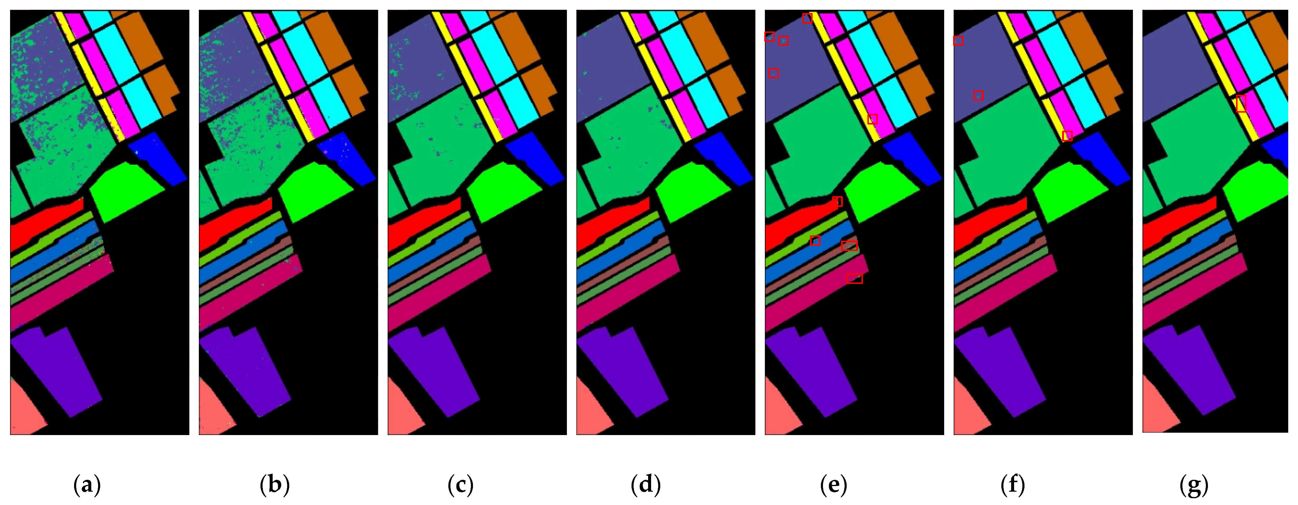
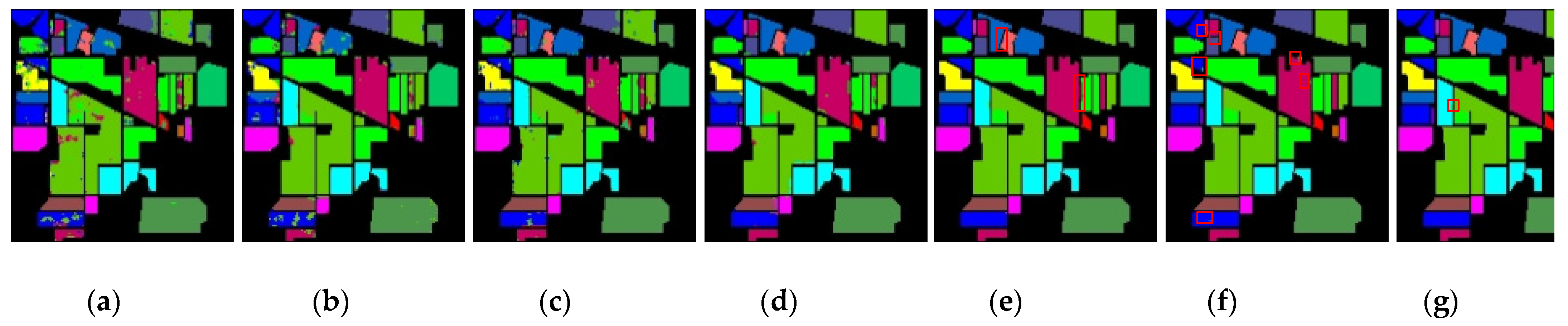
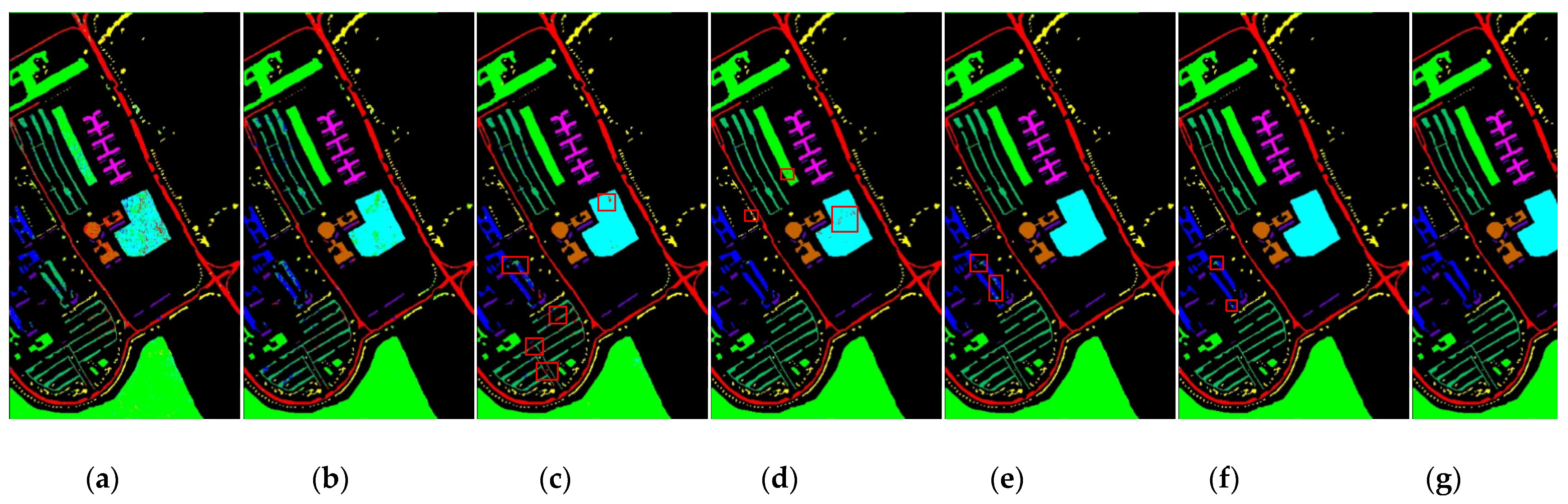
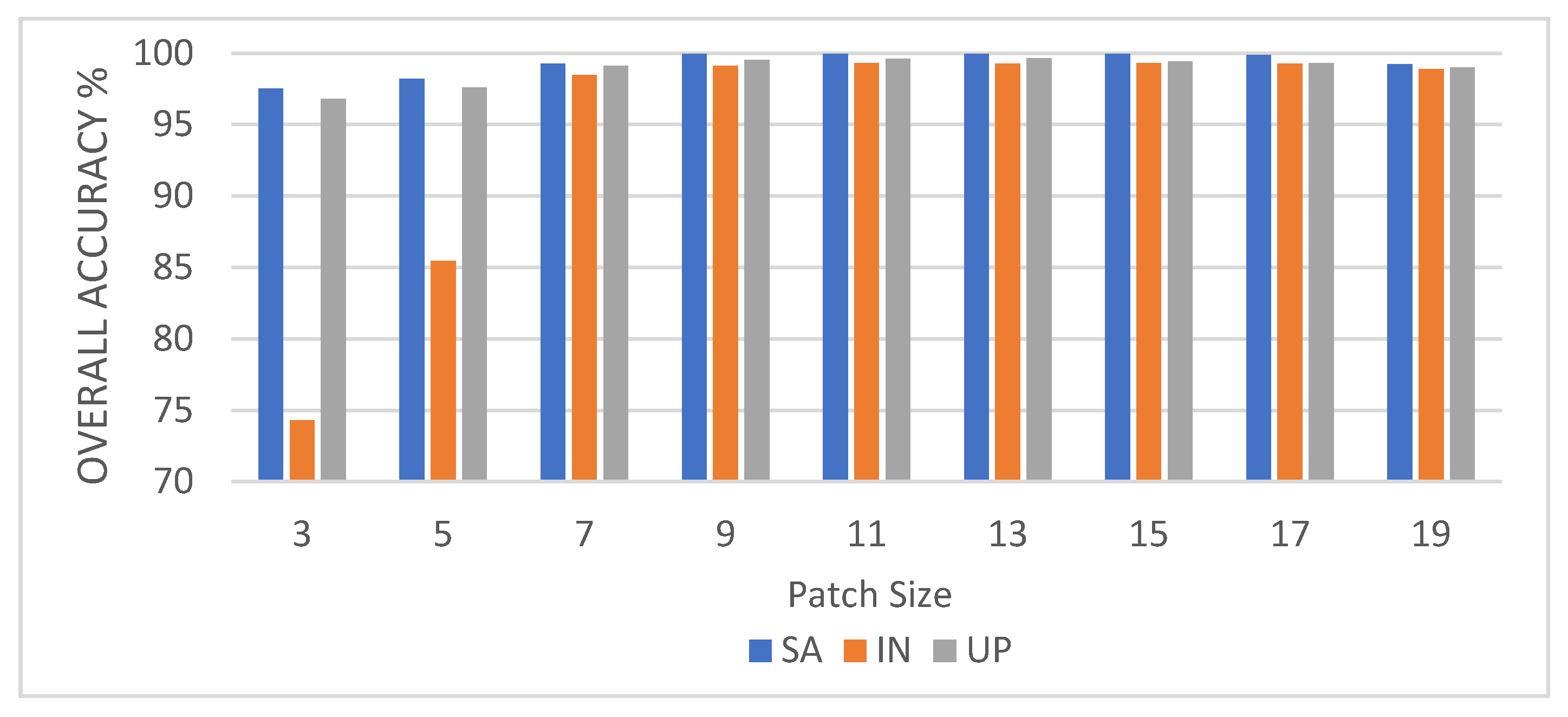
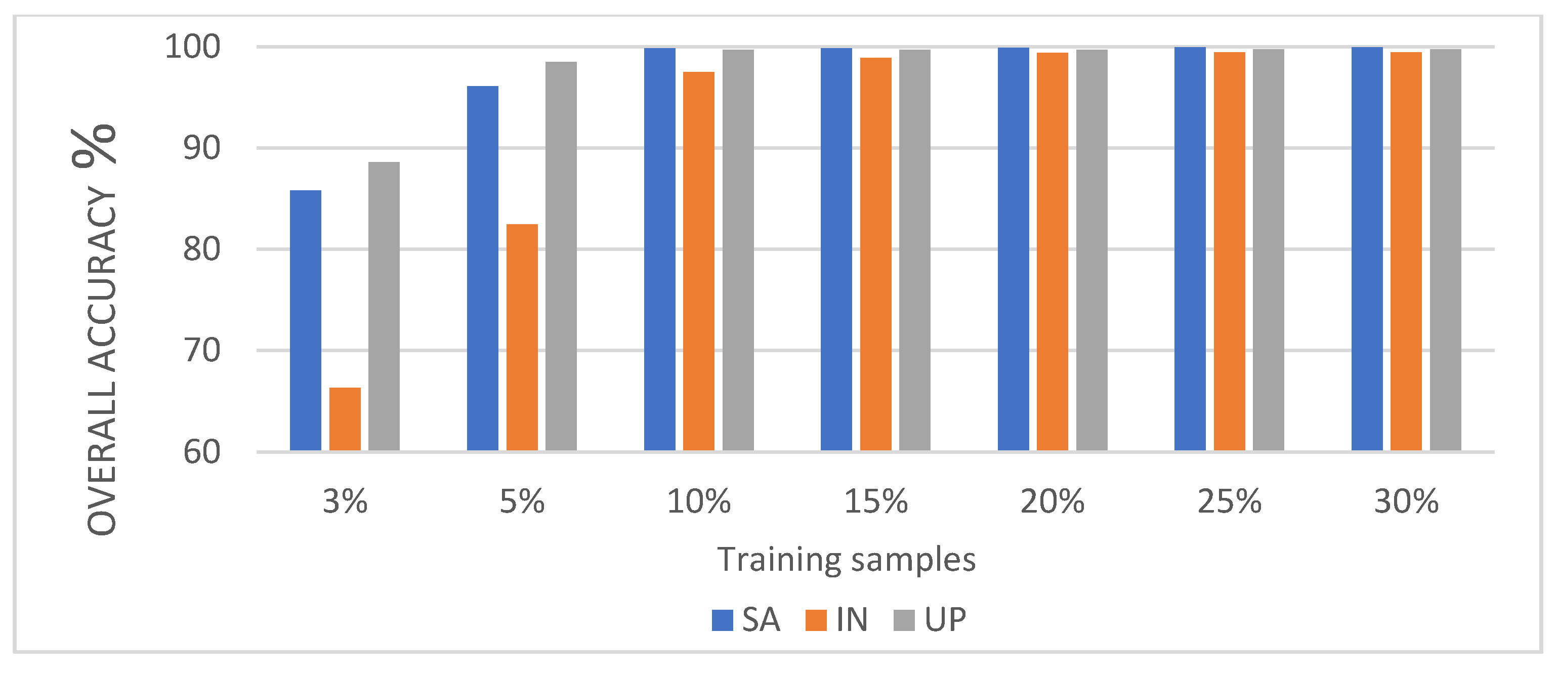
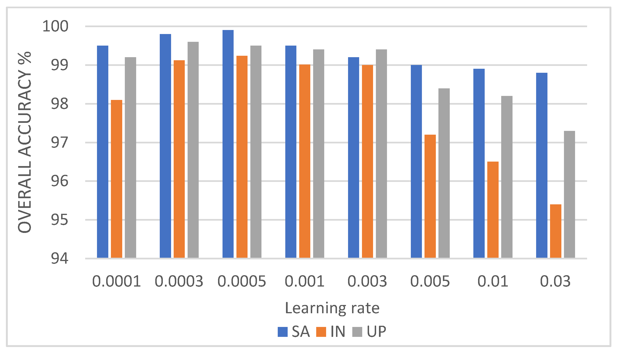
In this study, we propose a network model called 3DSA-MFN for the HSI classification task. The network includes a three-dimensional multi-head attention mechanism, multiscale feature fusion, and other modules. We first use the PCA algorithm to reduce the dimensionality of the spectrum and remove noisy and redundant data. In the feature extraction stage, we first use the multi-scale feature fusion module to first extract the feature information of HSI from different scales. Then, we generalize the multi-head self-attention from two-dimensional to three-dimensional and effectively improve it so that it can fully utilize the input matrix contextual information. Then, we use the improved 3D-MHSA to improve the convolutional neural network and get the 3DCOV_attention module. This module establishes the remote dependency while extracting local features, which can simultaneously improve the local receptive field, capture long-distance interactions, and improve the classification performance of the model. To test the effectiveness of the proposed method, experiments were conducted on three public datasets. Compared to methods such as SVM, 3D-CNN, SSAN, SSRN, HSI-BERT, and SAT, 3DSA-MFN achieved the best classification performance on the SA and UP datasets. For the IN dataset, the classification performance is slightly lower than that of HSI-BERT and achieved a classification performance comparable to that of SAT. Specifically, for the SA, IN, and UP datasets, 3DSA-MFN achieved OA values of 99.92%, 99.52%, and 99.77%, respectively, and AA values of 99.84%, 99.32%, and 99.68%, respectively. In future work, we will focus on optimizing the attention mechanism in HSI classification tasks and classifying small samples of HSIs.

References

1. Zhou, K.; Cheng, T.; Deng, X.; Yao, X.; Tian, Y.; Zhu, Y.; Cao, W. Assessment of spectral variation between rice canopy components using spectral feature analysis of near-ground hyperspectral imaging data. In Proceedings of the 8th Workshop on Hyperspectral Image and Signal Processing: Evolution in Remote Sensing (WHISPERS), Los Angeles, CA, USA, 21–24 August 2016. [Google Scholar]
2. Heldens, W.; Esch, T.; Heiden, U. Supporting urban micro climate modelling with airborne hyperspectral data. In Proceedings of the 32nd annual IEEE International Geoscience and Remote Sensing Symposium, Munich, Germany, 22–27 July 2012; pp. 1598–1601. [Google Scholar]
3. Yang, X.; Yu, Y. Estimating soil salinity under various moisture conditions: An experimental study. IEEE Trans. Geosci. Remote Sens. 2017, 55, 2525–2533. [Google Scholar] [CrossRef]
4. Zhong, Y.; Wang, X.; Xu, Y.; Wang, S.; Jia, T.; Hu, X.; Zhao, J.; Wei, L.; Zhang, L. Mini-UAV-borne hyperspectral remote sensing: From observation and processing to applications. IEEE Geosci. Remote Sens. Mag. 2018, 6, 46–62. [Google Scholar] [CrossRef]
5. Zhang, X.; Sun, Y.; Shang, K.; Zhang, L.; Wang, S. Crop classification based on feature band set construction and object-oriented approach using hyperspectral images. IEEE J. Sel. Top. Appl. Earth Observ. Remote Sens. 2016, 9, 4117–4128. [Google Scholar] [CrossRef]
6. Yokoya, N.; Chan, J.C.W.; Segl, K. Potential of resolution enhanced hyperspectral data for mineral mapping using simulated EnMAP and Sentinel-2 images. Remote Sens. 2016, 8, 172. [Google Scholar] [CrossRef] [Green Version]
7. Pandey, P.; Payn, K.G.; Lu, Y.; Heine, A.J.; Walker, T.D.; Acosta, J.J.; Young, S. Hyperspectral Imaging Combined with Machine Learning for the Detection of Fusiform Rust Disease Incidence in Loblolly Pine Seedlings. Remote Sens. 2021, 13, 3595. [Google Scholar] [CrossRef]
8. Vaglio Laurin, G.; Chan, J.C.; Chen, Q.; Lindsell, J.A.; Coomes, D.A.; Guerriero, L.; Frate, F.D.; Miglietta, F.; Valentini, R. Biodiversity Mapping in a Tropical West African Forest with Airborne Hyperspectral Data. PLoS ONE. 2014, 9, e97910. [Google Scholar] [CrossRef] [PubMed]
9. Ma, L.; Crawford, M.M.; Tian, J. Local Manifold Learning-Based k -Nearest-Neighbor for Hyperspectral Image. IEEE Trans. Geosci. Remote Sens. 2010, 48, 4099–4109. [Google Scholar]
10. Kang, X.; Li, S.; Benediktsson, J.A. Spectral–spatial hyperspectral image classification with edge-preserving filtering. IEEE Trans. Geosci. Remote Sens. 2014, 52, 2666–2677. [Google Scholar] [CrossRef]
11. Liu, J.; Wu, Z.; Wei, Z.; Xiao, L.; Sun, L. Spatial-spectral kernel sparse representation for hyperspectral image classification. IEEE J. Sel. Top. Appl. Earth Obs. Remote Sens. 2013, 6, 2462–2471. [Google Scholar] [CrossRef]
12. Zhang, Y.; Cao, G.; Li, X.; Wang, B.; Fu, P. Active Semi-Supervised Random Forest for Hyperspectral Image Classification. Remote Sens. 2019, 11, 2974. [Google Scholar] [CrossRef] [Green Version]
13. Cariou, C.; Chehdi, K. Unsupervised Nearest Neighbors Clustering With Application to Hyperspectral Images. IEEE J. Sel. Top. Signal. Process. 2015, 9, 1105–1116. [Google Scholar] [CrossRef] [Green Version]
14. Haut, J.M.; Paoletti, M.; Plaza, J.; Plaza, A. Cloud implementation of the k-means algorithm for hyperspectral image analysis. J. Supercomput. 2017, 73, 514–529. [Google Scholar] [CrossRef]
15. Wang, Q.; Lin, J.; Yuan, Y. Salient Band Selection for Hyperspectral Image Classification via Manifold Ranking. IEEE Trans. Neural Netw. Learn. Syst. 2016, 27, 1279–1289. [Google Scholar] [CrossRef] [PubMed]
16. Yuan, Y.; Lin, J.; Wang, Q. Hyperspectral Image Classification via Multitask Joint Sparse Representation and Stepwise MRF Optimization. IEEE Trans. Cybern. 2016, 46, 2966–2977. [Google Scholar] [CrossRef]
17. Chen, Y.; Zhao, X.; Jia, X. Spectral–Spatial Classification of Hyperspectral Data Based on Deep Belief Network. IEEE J. Sel. Top. Appl. Earth Obs. Remote Sens. 2015, 8, 2381–2392. [Google Scholar] [CrossRef]
18. Zhao, C.; Wan, X.; Yan, Y. Spectral-spatial classification of hyperspectral images based on joint bilateral filter and stacked sparse autoencoder. J. Appl. Remote Sens. 2017, 1, 1–5. [Google Scholar] [CrossRef]
19. Deng, D.; Xue, Y.; Liu, X.; Li, C.; Tao, D. Active Transfer Learning Network: A Unified Deep Joint Spectral–Spatial Feature Learning Model for Hyperspectral Image Classification. IEEE Trans. Geosci. Remote Sens. 2019, 57, 1741–1754. [Google Scholar] [CrossRef] [Green Version]
20. Cao, X.; Zhou, F.; Xu, l.; Meng, D.; Xu, Z.; Paisley, J. Hyperspectral image classification with markov random fields and a convolutional neural network. IEEE Trans. Image Process 2018, 27, 2354–2367. [Google Scholar] [CrossRef] [Green Version]
21. Hao, S.; Wang, W.; Ye, Y.; Li, E.; Bruzzone, L. A deep network architecture for super-resolution-aided hyperspectral image classification with classwise loss. IEEE Trans. Geosci. Remote Sens. 2018, 56, 4650–4663. [Google Scholar] [CrossRef]
22. Pan, B.; Xu, X.; Shi, Z.; Zhang, N.; Luo, H.; Lan, X. DSSNet: A Simple Dilated Semantic Segmentation Network for Hyperspectral Imagery Classification. IEEE Geosci. Remote Sens. Lett. 2020, 17, 1968–1972. [Google Scholar] [CrossRef]
23. Li, X.; Ding, M.; Pižurica, A. Deep Feature Fusion via Two-Stream Convolutional Neural Network for Hyperspectral Image Classification. IEEE Trans. Geosci. Remote Sens. 2020, 58, 2615–2629. [Google Scholar] [CrossRef] [Green Version]
24. Yang, X.F.; Ye, Y.M.; Li, X.T.; Lau, R.Y.K.; Zhang, X.F.; Huang, X.H. Hyperspectral Image Classification With Deep Learning Models. IEEE Trans. Geosci. Remote Sens. 2018, 56, 5408–5423. [Google Scholar] [CrossRef]
25. Sun, H.; Zheng, X.; Lu, X.; Wu, S. Spectral–Spatial Attention Network for Hyperspectral Image Classification. IEEE Trans. Geosci. Remote. Sens. 2020, 58, 3232–3245. [Google Scholar] [CrossRef]
26. Zhu, Z.; Luo, Y.; Qi, G.; Meng, J.; Li, Y.; Mazur, N. Remote Sensing Image Defogging Networks Based on Dual Self-Attention Boost Residual Octave Convolution. Remote Sens. 2021, 13, 3104. [Google Scholar] [CrossRef]
27. Zhu, M.; Jiao, L.; Liu, L.; Yang, S.; Wang, J. Residual Spectral–Spatial Attention Network for Hyperspectral Image Classification. IEEE Trans. Geosci. Remote Sens. 2021, 59, 449–462. [Google Scholar] [CrossRef]
28. Li, L.; Yin, J.; Jia, X.; Li, S.; Han, B. Joint Spatial–Spectral Attention Network for Hyperspectral Image Classification. IEEE Geosci. Remote. Sens. Lett. 2021, 18, 1816–1820. [Google Scholar] [CrossRef]
29. Qing, Y.; Liu, W. Hyperspectral Image Classification Based on Multi-Scale Residual Network with Attention Mechanism. Remote Sens. 2021, 13, 335. [Google Scholar] [CrossRef]
30. Lu, Z.; Xu, B.; Sun, L.; Zhan, T.; Tang, S. 3-D Channel and Spatial Attention Based Multiscale Spatial–Spectral Residual Network for Hyperspectral Image Classification. IEEE J. Sel. Top. Appl. Earth Obs. Remote. Sens. 2020, 13, 4311–4324. [Google Scholar] [CrossRef]
31. Song, M.; Shang, X.; Chang, C.I. 3-D Receiver Operating Characteristic Analysis for Hyperspectral Image Classification. IEEE Trans. Geosci. Remote. Sens. 2020, 58, 8093–8115. [Google Scholar] [CrossRef]
32. Tang, X.; Meng, F.; Zhang, X.; Cheung, Y.M.; Ma, J.; Liu, F.; Jiao, L. Hyperspectral Image Classification Based on 3-D Octave Convolution With Spatial–Spectral Attention Network. IEEE Trans. Geosci. Remote. Sens. 2021, 59, 2430–2447. [Google Scholar] [CrossRef]
33. Farooque, G.; Xiao, L.; Yang, J.; Sargano, A.B. Hyperspectral Image Classification via a Novel Spectral–Spatial 3D ConvLSTM-CNN. Remote Sens. 2021, 13, 4348. [Google Scholar] [CrossRef]
34. Yan, H.; Wang, J.; Tang, L.; Zhang, E.; Yan, K.; Yu, K.; Peng, J. A 3D Cascaded Spectral–Spatial Element Attention Network for Hyperspectral Image Classification. Remote Sens. 2021, 13, 2451. [Google Scholar] [CrossRef]
35. Yin, J.; Qi, C.; Chen, Q.; Qu, J. Spatial-Spectral Network for Hyperspectral Image Classification: A 3-D CNN and Bi-LSTM Framework. Remote Sens. 2021, 13, 2353. [Google Scholar] [CrossRef]
36. He, J.; Zhao, l.; Yang, H.; Zhang, M.; Li, W. HSI-BERT: Hyperspectral Image Classification Using the Bidirectional Encoder Representation From Transformers. IEEE Trans. Geosci. Remote. Sens. 2020, 58, 165–178. [Google Scholar] [CrossRef]
37. Qing, Y.; Liu, W.; Feng, L.; Gao, W. Improved Transformer Net for Hyperspectral Image Classification. Remote Sens. 2021, 13, 2216. [Google Scholar] [CrossRef]
38. He, X.; Chen, Y. Optimized Input for CNN-Based Hyperspectral Image Classification Using Spatial Transformer Nework. IEEE Geosci. Remote. Sens. Lett. 2019, 16, 1884–1888. [Google Scholar] [CrossRef]
39. Zhong, Z.; Li, Y.; Ma, L.; Li, J.; Zheng, S.W. Spectral-Spatial Transformer Network for Hyperspectral Image Classification: A Factorized Architecture Search Framework. IEEE Trans. Geosci. Remote. Sens. 2021, 60, 1–15. [Google Scholar] [CrossRef]
40. Gao, L.; Liu, H.; Yang, M.; Chen, L.; Wan, Y.; Xiao, Z.; Qian, Y. STransFuse: Fusing Swin Transformer and Convolutional Neural Network for Remote Sensing Image Semantic Segmentation. IEEE J. Sel. Top. Appl. Earth Obs. Remote. Sens. 2021, 14, 10990–11003. [Google Scholar] [CrossRef]
41. Szegedy, C.; Ioffe, S.; Vanhoucke, V.; Alemi, A. Inception-v4, Inception-ResNet and the Impact of Residual Connections on Learning. Available online: https://www.aaai.org/ocs/index.php/AAAI/AAAI17/paper/viewPaper/14806 (accessed on 7 January 2022).
42. Chen, L.C.; Zhu, Y.; Papandreou, G.; Schroff, F.; Adam, H. Encoder-Decoder with Atrous Separable Convolution for Semantic Image Segmentation. Available online: https://openaccess.thecvf.com/content_ECCV_2018/html/Liang-Chieh_Chen_Encoder-Decoder_with_Atrous_ECCV_2018_paper.html (accessed on 7 January 2022).
43. Zhao, H.; Shi, J.; Qi, X.; Wang, X.; Jia, J. Pyramid Scene Parsing Network. Available online: https://openaccess.thecvf.com/content_cvpr_2017/html/Zhao_Pyramid_Scene_Parsing_CVPR_2017_paper.html (accessed on 7 January 2022).
44. Chen, C.F.; Fan, Q.; Mallinar, N.; Sercu, T.; Feri, R. Big-Little-Net: An Efficient Multi-Scale Feature Representation for Visual and Speech Recognition. Available online: https://arxiv.org/abs/1807.03848 (accessed on 7 January 2022).
45. Bahdanau, D.; Cho, K.; Bengio, Y. Neural Machine Translation by Jointly learning to Align and Translate. Available online: https://arxiv.org/abs/1409.0473 (accessed on 7 January 2022).
46. Devlin, J.; Chang, M.W.; Lee, K.; Toutanova, K. BERT: Pre-Training of Deep Bidirectional Transformers for Language Understanding. Available online: https://arxiv.org/abs/1810.04805 (accessed on 7 January 2022).
47. Dai, Z.; Yang, Z.; Yang, Y.; Carbonell, J.; Le, Q.V.; Salakhutdinov, R. Transformer-XL: Attentive Language Models beyond a Fixed-Length Context. Available online: https://arxiv.org/abs/1901.02860 (accessed on 7 January 2022).
48. Vaswani, A.; Shazeer, N.; Parmar, N.; Uszkoreit, J.; Jones, L.; Gomez, A.N.; Kaiser, L.; Polosukhin, I. Attention is All You Need. Available online: https://proceedings.neurips.cc/paper/2017/hash/3f5ee243547dee91fbd053c1c4a845aa-Abstract.html (accessed on 7 January 2022).
49. Yang, Z.; Dai, Z.; Yang, Y.; Carbonell, J.; Salakhutdinov, R.; Le, Q.V. XLNet: Generalized Autoregressive Pretraining for Language Understanding. Available online: https://proceedings.neurips.cc/paper/2019/hash/dc6a7e655d7e5840e66733e9ee67cc69-Abstract.html (accessed on 7 January 2022).
50. Dosovitskiy, A.; Beyer, L.; Kolesnikov, A.; Weissenborn, D.; Zhai, X.; Unterthiner, T.; Dehghani, M.; Minderer, M.; Heigold, G.; Gelly, S.; et al. An Image is Worth16 x 16 Words: Transformers for Image Recognition at scale. Available online: https://arxiv.org/abs/2010.11929 (accessed on 7 January 2022).
51. Touvron, H.; Cord, M.; Douze, M.; Massa, F.; Sablayrolles, A.; Jégou, H. Training Data-Efficient Image Transformers & Distillation through Attention. Available online: https://proceedings.mlr.press/v139/touvron21a (accessed on 7 January 2022).
52. Zhu, X.; Su, W.; Lu, L.; Li, B.; Wang, X.; Dai, J. Deformable detr: Deformable Transformers for end-to-end Object Detection. Available online: https://arxiv.org/abs/2010.04159 (accessed on 7 January 2022).
53. Carion, N.; Massa, F.; Synnaeve, G.; Usunier, N.; Kirillov, A.; Zagoruyko, S. End-to-End Object Detection with Transformers. Available online: https://link.springer.com/chapter/10.1007/978-3-030-58452-8_13 (accessed on 7 January 2022).
54. Zheng, S.; Lu, J.; Zhao, H.; Zhu, X.; Luo, Z.; Wang, Y.; Fu, Y.; Feng, J.; Xiang, T.; Torr, P.H.S.; et al. Rethinking Semantic Segmentation from a Sequence-to-Sequence Perspective with Transformers. Available online: https://openaccess.thecvf.com/content/CVPR2021/html/Zheng_Rethinking_Semantic_Segmentation_From_a_Sequence-to-Sequence_Perspective_With_Transformers_CVPR_2021_paper.html (accessed on 7 January 2022).
55. Chen, X.; Wang, H.; Ni, B. X-volution: On the Unification of Convolution and Self-Attention. Available online: https://arxiv.org/abs/2106.02253 (accessed on 7 January 2022).
56. Li, Y.; Yao, T.; Pan, Y.; Mei, T. Contextual Transformer Networks for Visual Recognition. Available online: https://arxiv.org/abs/2107.12292 (accessed on 7 January 2022).
57. Wu, H.; Xiao, B.; Codella, N.; Liu, H.; Dai, H.; Yuan, L.; Zhang, L. CvT: Introducing Convolutions to Vision Transform ers. Available online: https://openaccess.thecvf.com/content/ICCV2021/html/Wu_CvT_Introducing_Convolutions_to_Vision_Transformers_ICCV_2021_paper.html (accessed on 7 January 2022).
58. Shaw, P.; Uszkoreit, J.; Vaswani, A. Self-Attention with Relative Position Representations. Available online: https://arxiv.org/abs/1803.02155 (accessed on 7 January 2022).
59. Guo, J.; Wu, K.H.; Xu, C.; Tang, Y.; Xu, C.; Wang, Y. CMT: Convolutional Neural Networks Meet Vision Transformers. Available online: https://arxiv.org/abs/2107.06263 (accessed on 7 January 2022).
60. Qing, Y.; Liu, W.; Feng, L.; Gao, W. Improved YOLO Network for Free-Angle Remote Sensing Target Detection. Remote Sens. 2021, 13, 2171. [Google Scholar] [CrossRef]
61. Fang, S.; LI, K.; Li, Z. S2ENet: Spatial-spectral Cross-Modal Enhancement Network for Classification of Hyperspectral and LiDAR Data. IEEE Geosci. Remote. Sens. Letters. 2022, 19, 1–5. [Google Scholar] [CrossRef]
62. Fang, S.; Li, K.; Shao, J.; Li, Z. SNUNet-CD: A Densely Connected Siamese Network for Change Detection of VHR Images. IEEE Geosci. Remote. Sens. Letters. 2022, 19, 1–5. [Google Scholar] [CrossRef]
63. Yang, X.; Zhang, X.; Ye, Y.; Lau, R.Y.K.; Lu, S.; Li, X.; Huang, X. Synergistic 2D/3D Convolutional Neural Network for Hyperspectral Image Classification. Remote Sens. 2020, 12, 2033. [Google Scholar] [CrossRef]
64. Srinivas, A.; Lin, T.Y.; Parmar, N.; Shlens, J.; Abbeel, P.; Vaswani, A. Bottleneck Transformers for Visual Recognition. Available online: https://openaccess.thecvf.com/content/CVPR2021/html/Srinivas_Bottleneck_Transformers_for_Visual_Recognition_CVPR_2021_paper.html (accessed on 7 January 2022).
65. Vaswani, A.; Ramachandran, P.; Srinivas, A.; Parmar, N.; Hechtman, B.; Shlens, J. Scaling Local Self-Attention for Parameter Efficient Visual Backbones. Available online: https://openaccess.thecvf.com/content/CVPR2021/html/Vaswani_Scaling_Local_Self-Attention_for_Parameter_Efficient_Visual_Backbones_CVPR_2021_paper.html (accessed on 7 January 2022).
66. Liu, Z.; Lin, Y.; Cao, Y.; Hu, H.; Wei, Y.; Zhang, Z.; Lin, S.; Guo, B. Swin transformer: Hierarchical Vision Transformer Using Shifted Windows. Available online: https://openaccess.thecvf.com/content/ICCV2021/html/Liu_Swin_Transformer_Hierarchical_Vision_Transformer_Using_Shifted_Windows_ICCV_2021_paper.html (accessed on 7 January 2022).
67. Graham, G.; El-Nouby, A.; Touvron, H.; Stock, P.; Joulin, A.; Jégou, H.; Douze, M. Levit: A Vision Transformer in Convnet’s Clothing for Faster Inference. Available online: https://openaccess.thecvf.com/content/ICCV2021/html/Graham_LeViT_A_Vision_Transformer_in_ConvNets_Clothing_for_Faster_Inference_ICCV_2021_paper.html (accessed on 7 January 2022).
68. Yuan, L.; Chen, Y.; Wang, T.; Yu, W.; Shi, Y.; Tay, F.E.H.; Feng, J.; Yan, S. Tokens-to-Token vit: Training Vision Transformers from Scratch on Imagenet. Available online: https://openaccess.thecvf.com/content/ICCV2021/html/Yuan_Tokens-to-Token_ViT_Training_Vision_Transformers_From_Scratch_on_ImageNet_ICCV_2021_paper.html?ref=https://githubhelp.com (accessed on 7 January 2022).
69. Yuan, K.; Guo, S.; Liu, Z.; Zhou, A.; Yu, F.; Wu, W. Incorporating Convolution Designs into Visual Transformers. Available online: https://openaccess.thecvf.com/content/ICCV2021/html/Yuan_Incorporating_Convolution_Designs_Into_Visual_Transformers_ICCV_2021_paper.html (accessed on 7 January 2022).
70. Wang, W.; Xie, E.; Li, X.; Fan, D.P.; Song, K.; Liang, D.; Lu, T.; Luo, P.; Shao, L. Pyramid vision transformer: A versatile backbone for dense prediction without convolutions. Available online: https://openaccess.thecvf.com/content/ICCV2021/html/Wang_Pyramid_Vision_Transformer_A_Versatile_Backbone_for_Dense_Prediction_Without_ICCV_2021_paper.html (accessed on 7 January 2022).
71. Waske, S.; van der Linden, S.; Benediktsson, J.A.; Rabe, A.; Hostert, P. Sensitivity of support vector machines to random feature selection in classification of hyperspectral data. IEEE Trans. Geosci.Remote Sens. 2010, 48, 2880–2889. [Google Scholar] [CrossRef] [Green Version]
72. Chen, Y.; Jiang, H.; Li, C.; Jia, X.; Ghamisi, P. Deep Feature Extraction and Classification of Hyperspectral Images Based on Convolutional Neural Networks. IEEE Trans. Geosci. Remote Sens. 2016, 54, 6232–6251. [Google Scholar] [CrossRef] [Green Version]
73. Zhong, Z.; Li, J.; Luo, Z.; Chapman, M. Spectral–Spatial Residual Network for Hyperspectral Image Classification: A 3-D Deep Learning Framework. IEEE Trans. Geosci. Remote Sens. 2018, 56, 847–858. [Google Scholar] [CrossRef]
Figure 1. Proposed 3DSA-MFN network framework. The proposed method preprocesses the original data through dimensionality reduction and window clipping, then sends the processed data to multiscale feature fusion, 3DCOV_attention and other modules for feature extraction, and finally outputs the classification results over multiple fully connected layers.
Remotesensing 14 00742 g001
Figure 2. Multi-scale feature fusion module.
Remotesensing 14 00742 g002
Figure 3. Improved 3D multi-head self-attention.
Remotesensing 14 00742 g003
Figure 4. 3D Convolutional Neural Network with Self-Attention (3DCOV_attention).
Remotesensing 14 00742 g004
Figure 5. Salinas images: (a) pseudo-color image; (b) ground-truth labels.
Remotesensing 14 00742 g005
Figure 6. Indian Pines images: (a) pseudo-color image; (b) ground-truth labels.
Remotesensing 14 00742 g006
Figure 7. University of Pavia images: (a) pseudo-color image; (b) ground-truth labels.
Remotesensing 14 00742 g007
Figure 8. Overall classification accuracy per dataset under various patch sizes.
Remotesensing 14 00742 g008
Figure 9. Overall classification accuracy per dataset under various proportions of training samples.
Remotesensing 14 00742 g009
Figure 10. Overall classification accuracy per dataset under various learning rates.
Remotesensing 14 00742 g010
Figure 11. Overall accuracy curve of different models in SA dataset.
Remotesensing 14 00742 g011
Figure 12. Overall accuracy curve of different models in IN dataset.
Remotesensing 14 00742 g012
Figure 13. Overall accuracy curve of different models in UP dataset.
Remotesensing 14 00742 g013
Figure 14. The classification map on the SA dataset for (a) SVM, (b) 3D-CNN, (c) SSAN (d) SSRN, (e) HSI-BERT, (f) SAT, and (g) proposed 3DSA-MFN. Red boxes are used to mark non-obvious misclassifications and noise.
Remotesensing 14 00742 g014
Figure 15. The classification map on the IN dataset for (a) SVM, (b) 3D-CNN, (c) SSAN (d) SSRN, (e) HSI-BERT, (f) SAT, and (g) proposed 3DSA-MFN. Red boxes are used to mark non-obvious misclassifications and noise.
Remotesensing 14 00742 g015
Figure 16. The classification map on the UP dataset for (a) SVM, (b) 3D-CNN, (c) SSAN (d) SSRN, (e) HSI-BERT, (f) SAT, and (g) proposed 3DSA-MFN. Red boxes are used to mark non-obvious misclassifications and noise.
Remotesensing 14 00742 g016