
Evaluating Machine Learning and Remote Sensing in Monitoring NO2 Emission of Power Plants


Abstract
:
1. Introduction
2. Related Work
3. Materials and Methods
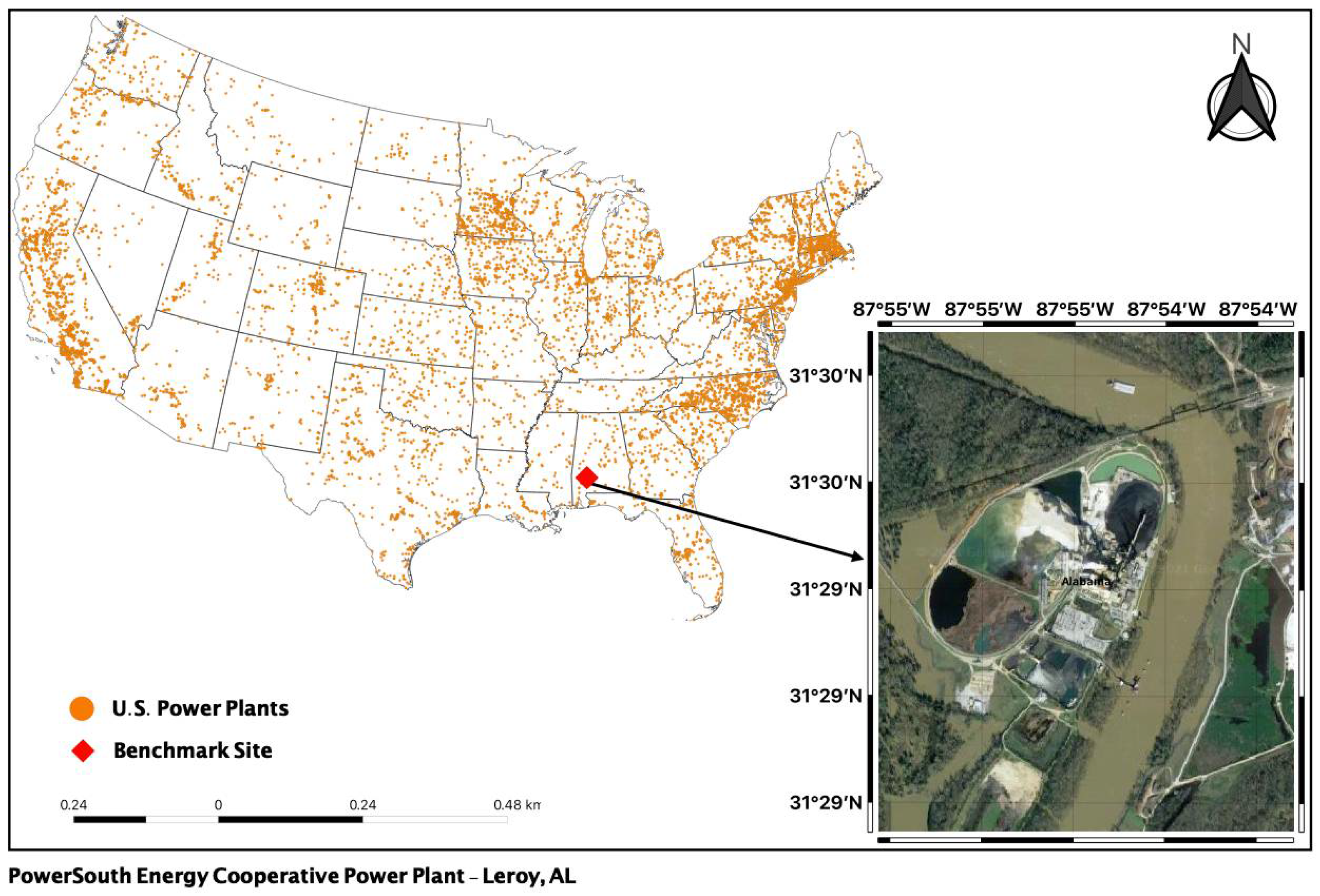
3.1. Study Area
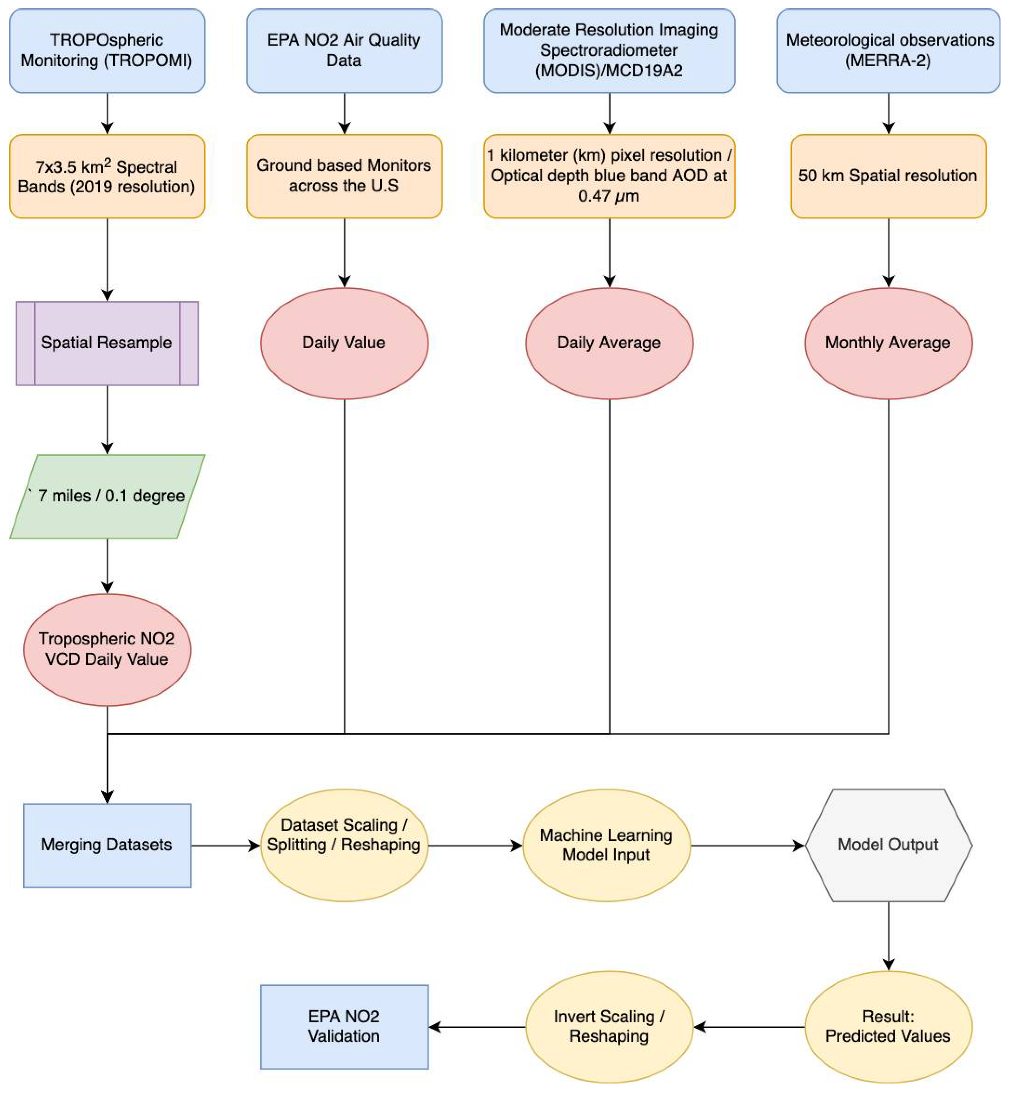
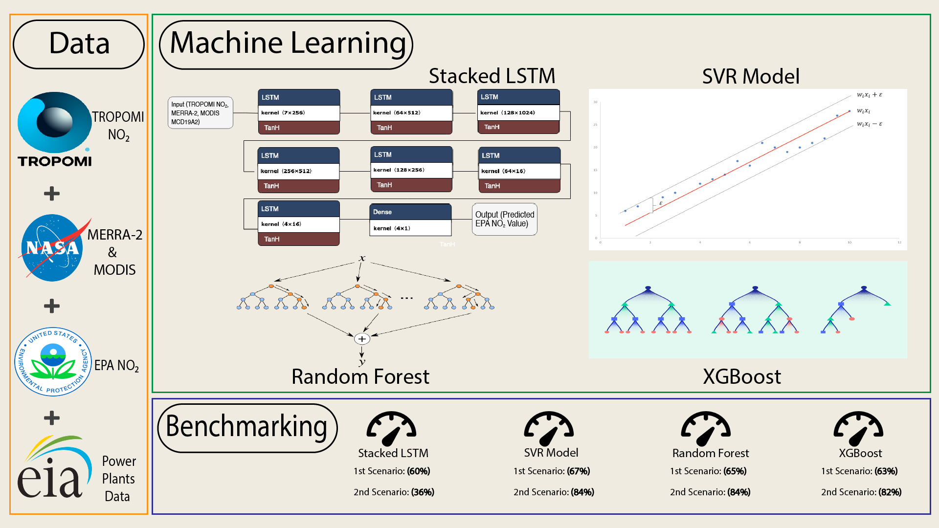
3.2. Data
3.2.1. TROPOMI Tropospheric NO2 Data
3.2.2. MERRA-2 Meteorology Data
3.2.3. EPA eGRID Data
3.2.4. U.S. Power Plants Data
3.2.5. MODIS MCD19A2
3.3. Preprocessing & Post-Processing
3.3.1. eGRID Data Preparation
3.3.2. TROPOMI Data Preparation
3.3.3. MCD19A2 Data Preparation
3.3.4. TROPOMI/EPA Value Pairs
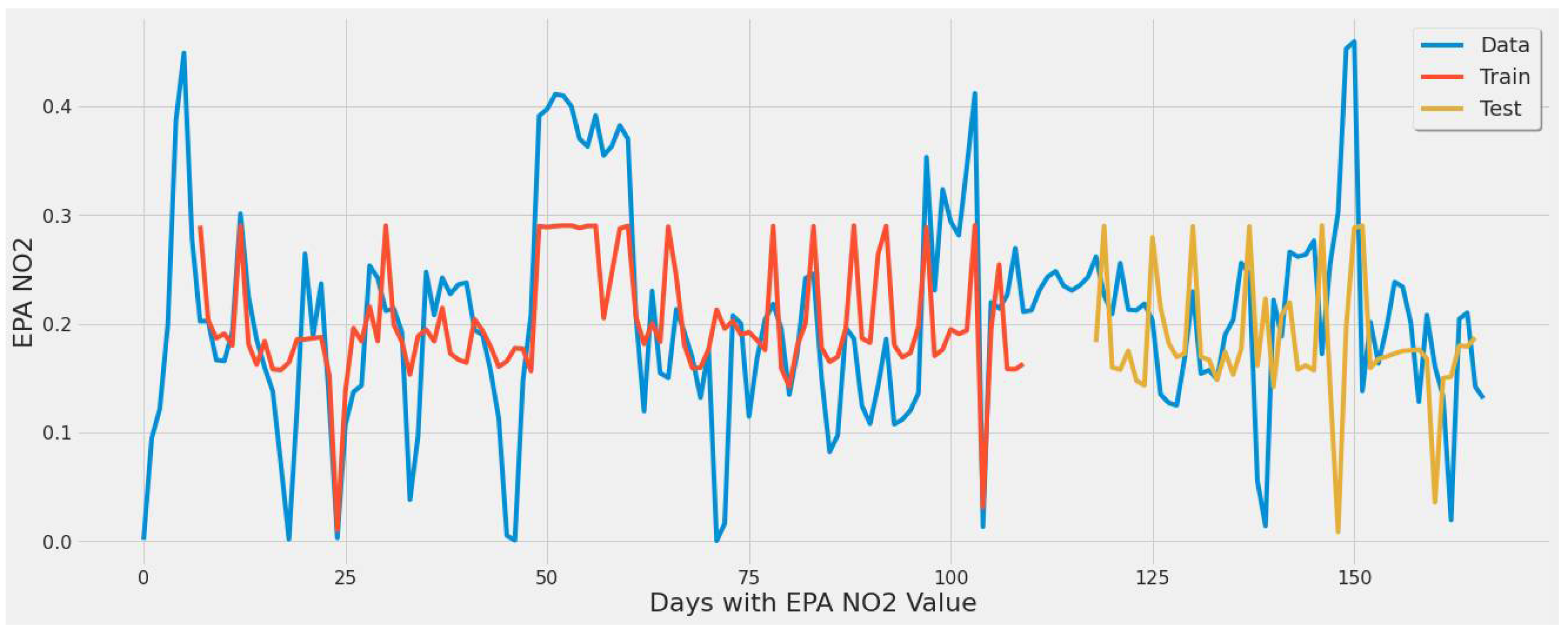
3.3.5. Dataset Preparation
3.4. Machine Learning Models
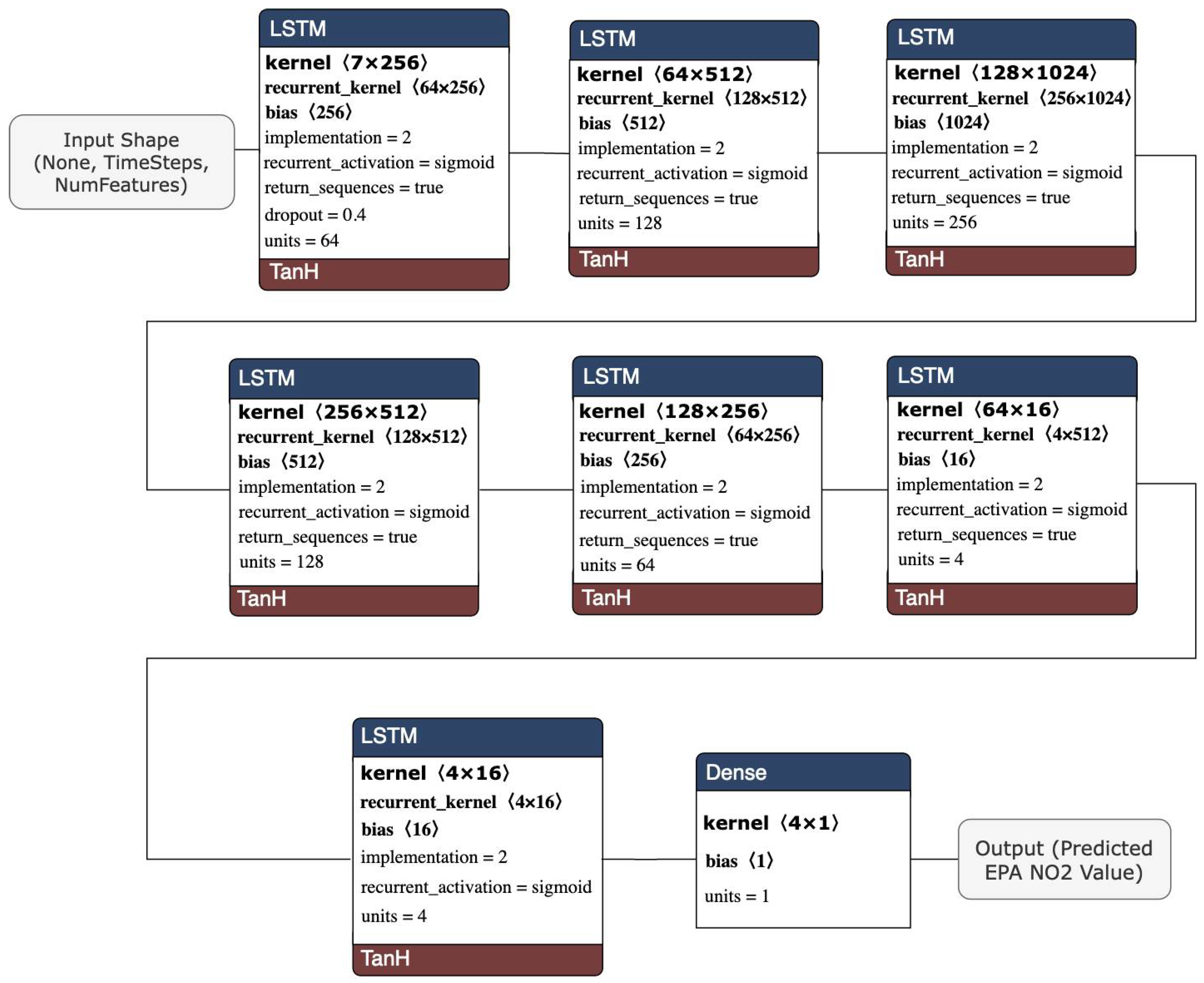
3.4.1. Long Short-Term Memory (LSTM)
- The first set only contained two features (EPA NO2, TROPOMI).
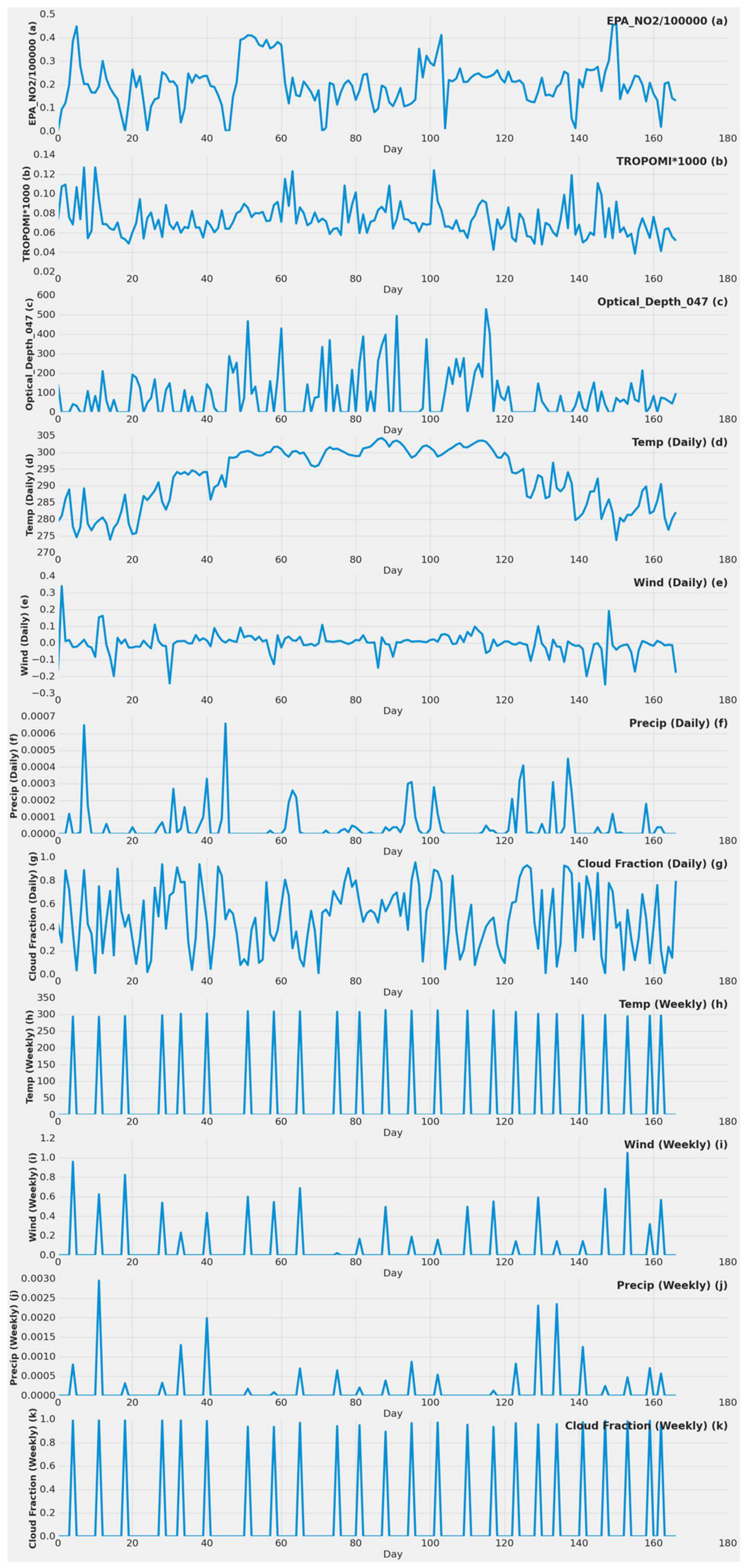
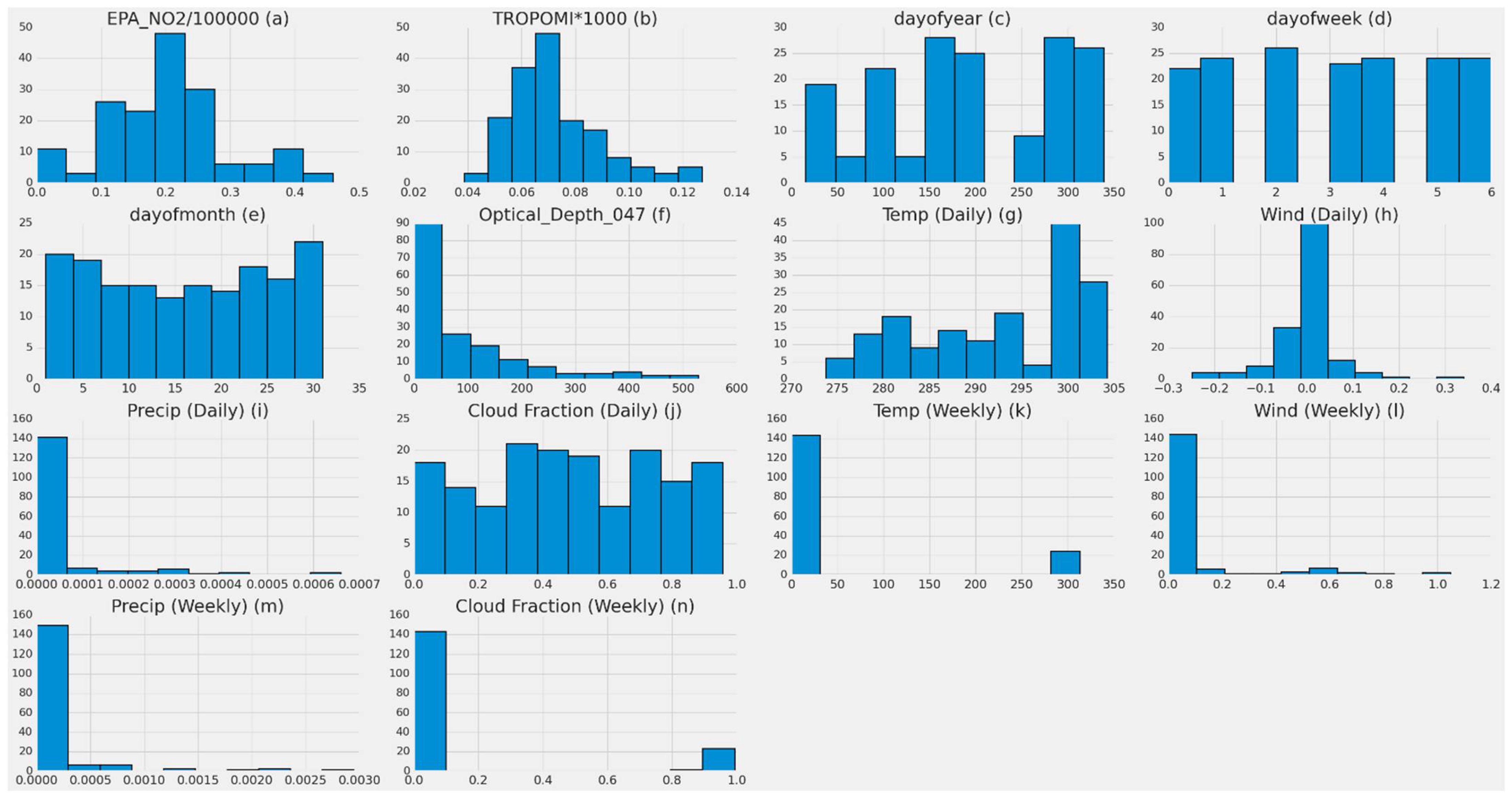
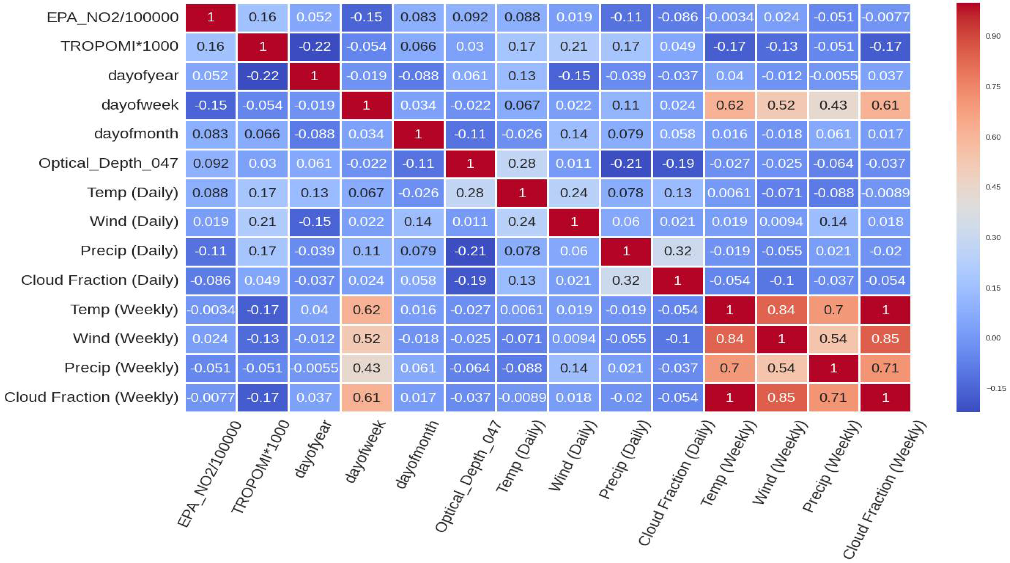
- The second input dataset included MERRA-2 (daily, weekly, monthly), TROPOMI NO2, and date features (EPA_NO2_10000, TROPOMI*1000, dayOfYear, dayOfWeek, dayOfMonth, MERRA-2 Wind, MERRA-2 Temp, MERRA-2 Precip, MERRA-2 Cloud Fraction).
- The third input set contained previously mentioned features and MCD19A2.
3.4.2. Support Vector Regression (SVR)
3.4.3. Random Forest
3.4.4. XGBoost
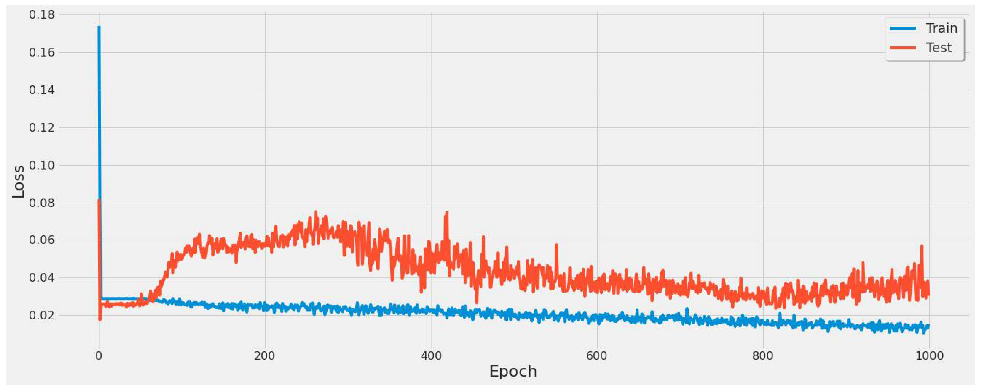
3.5. Model Training Error Metrics
3.6. Tools and Hardware
4. Experiments and Results
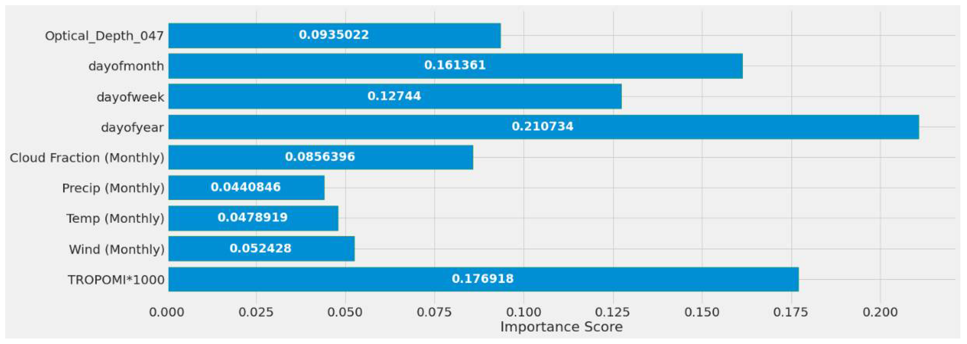
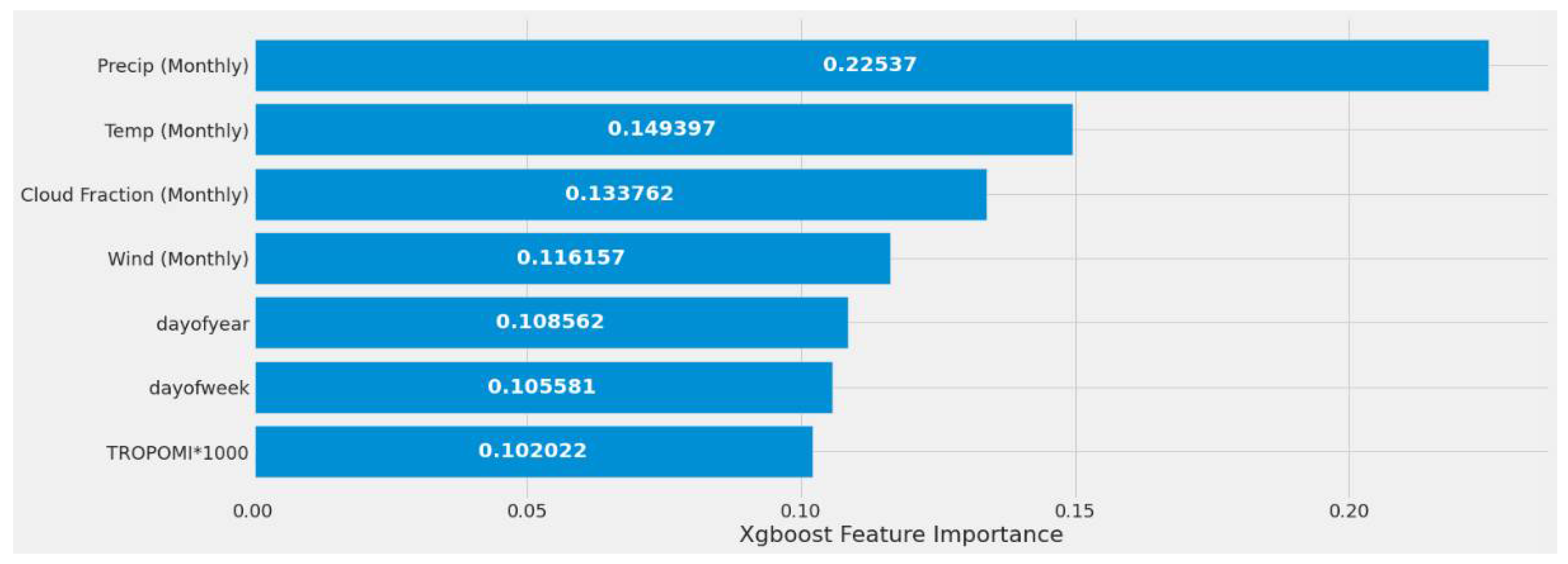
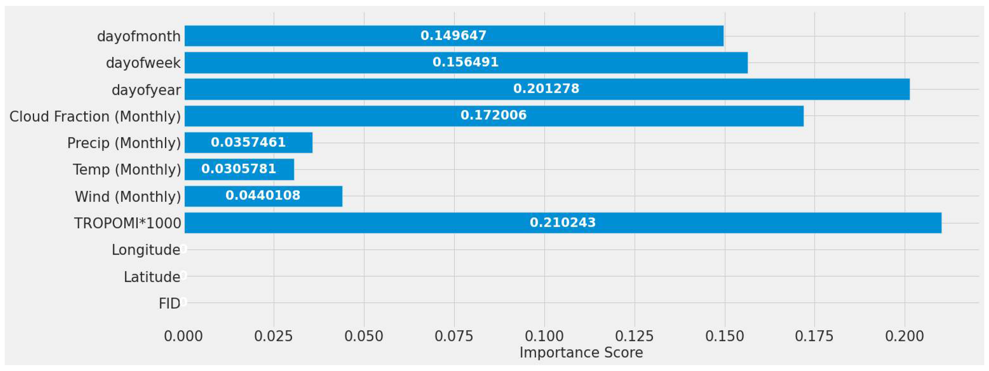
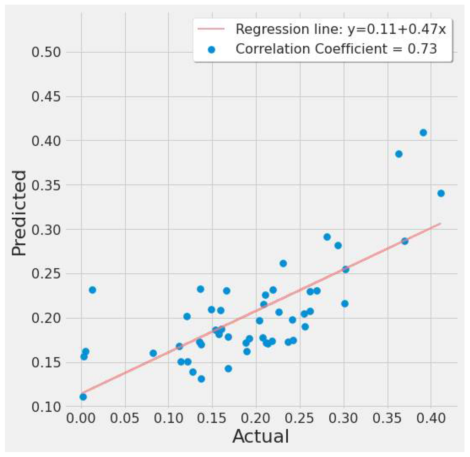
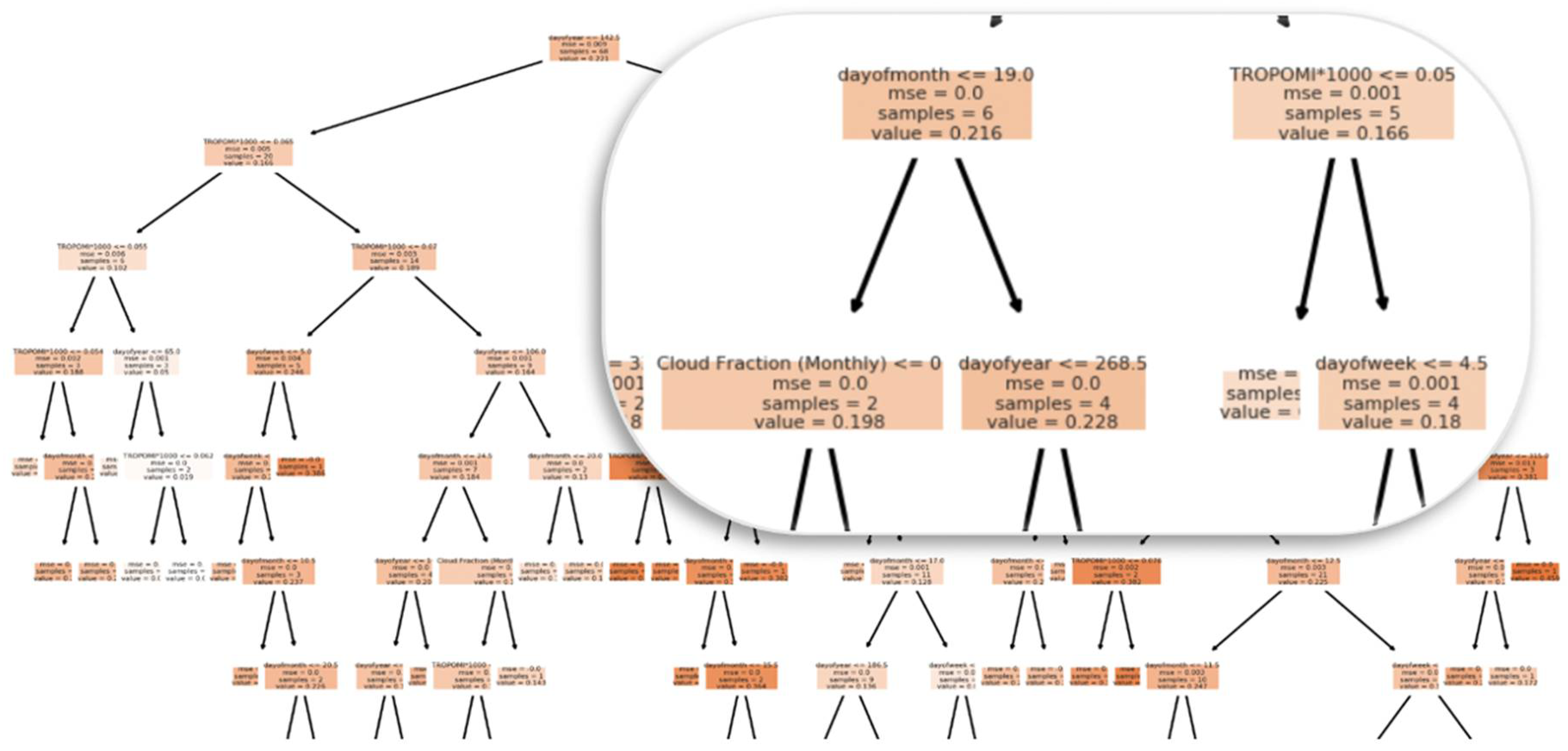
4.1. Feature Importance Results
4.2. Early Testing
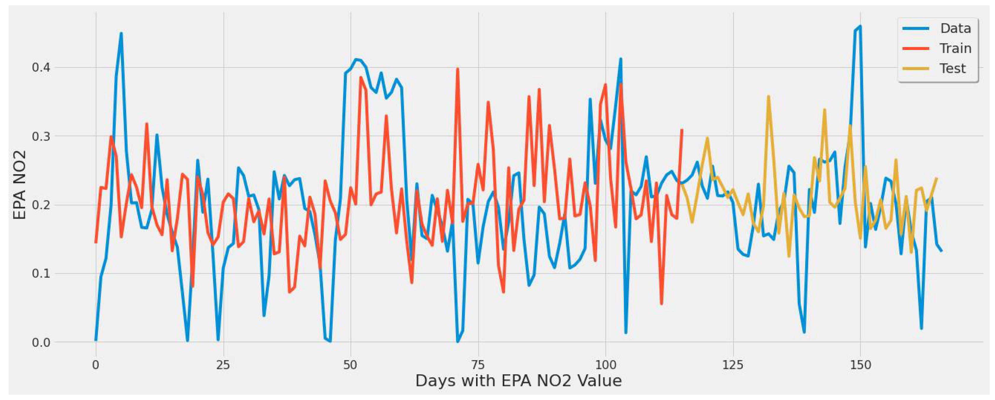
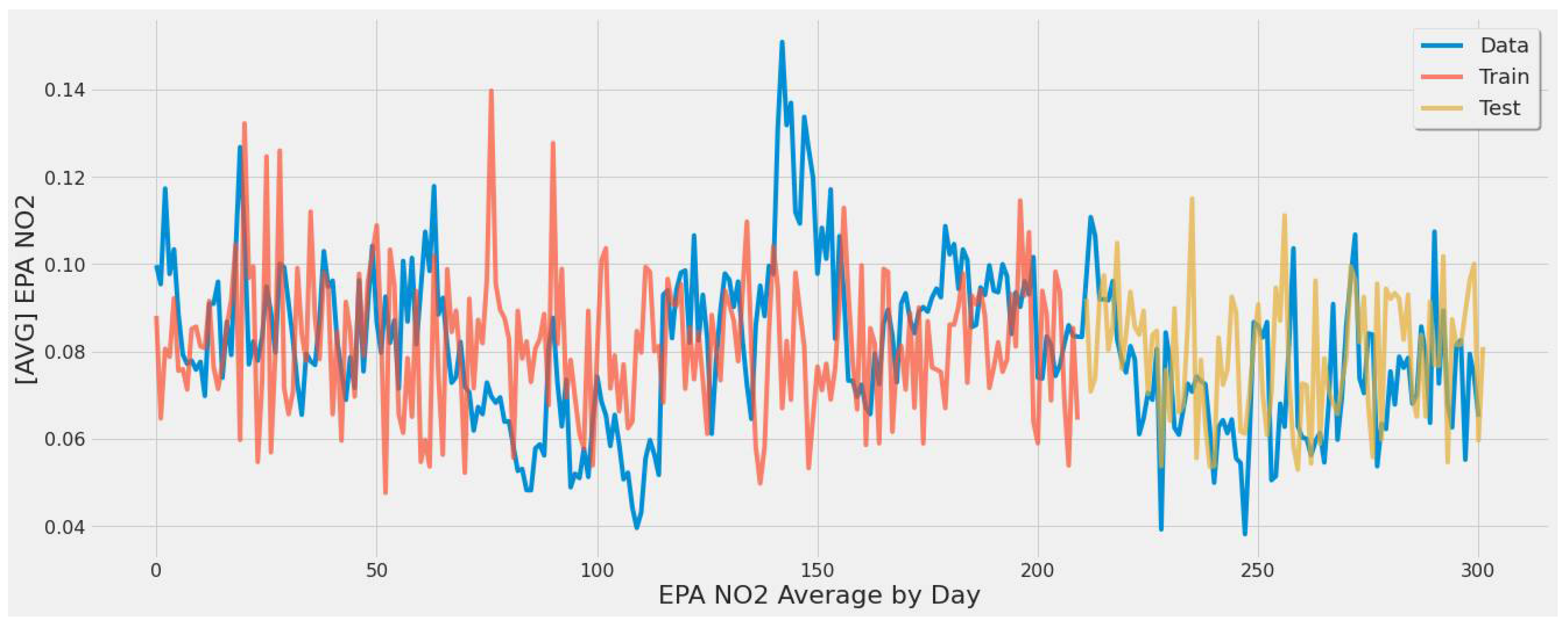
4.3. Improved ML Models
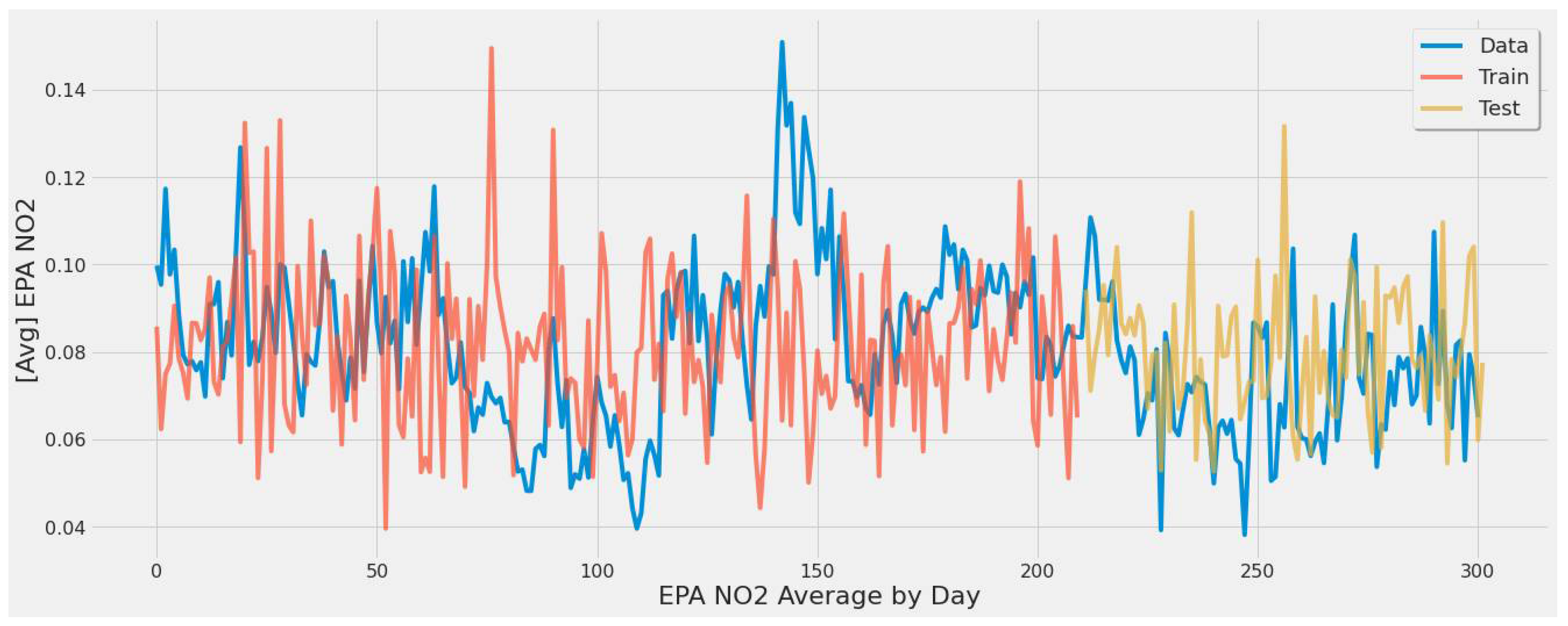
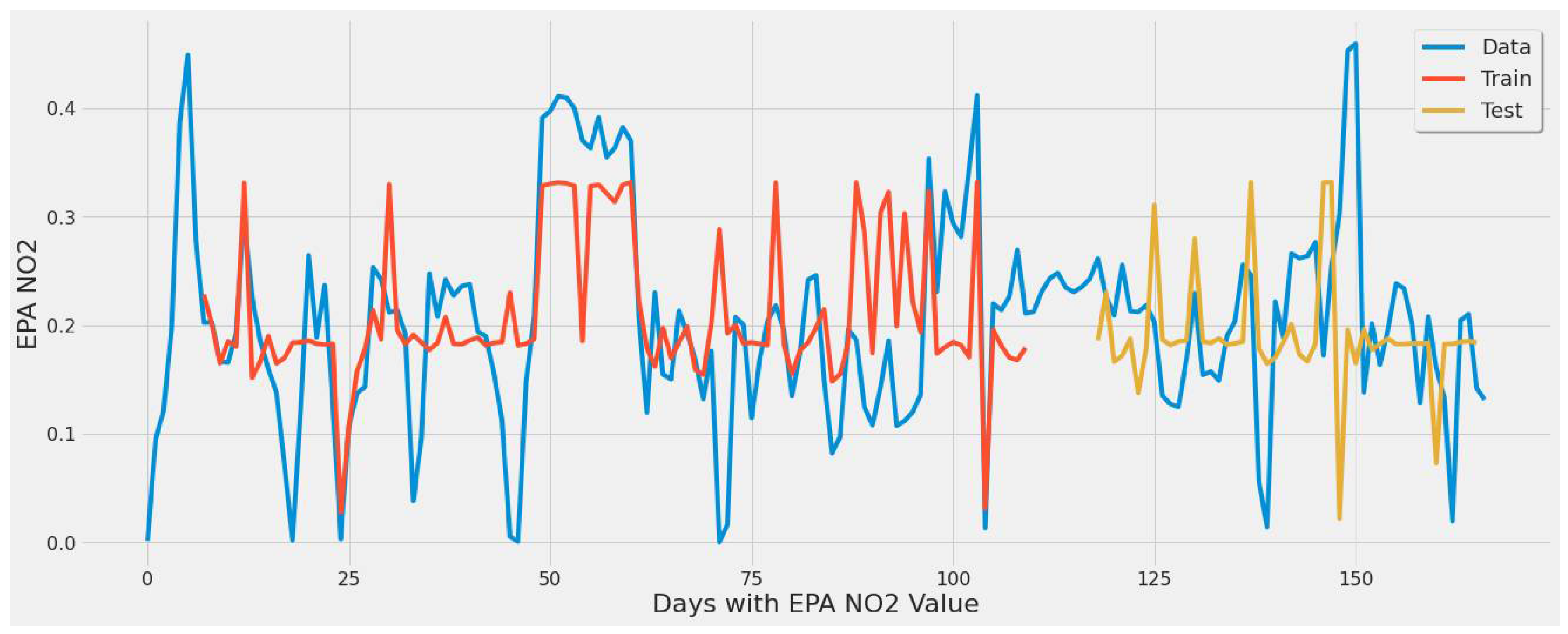
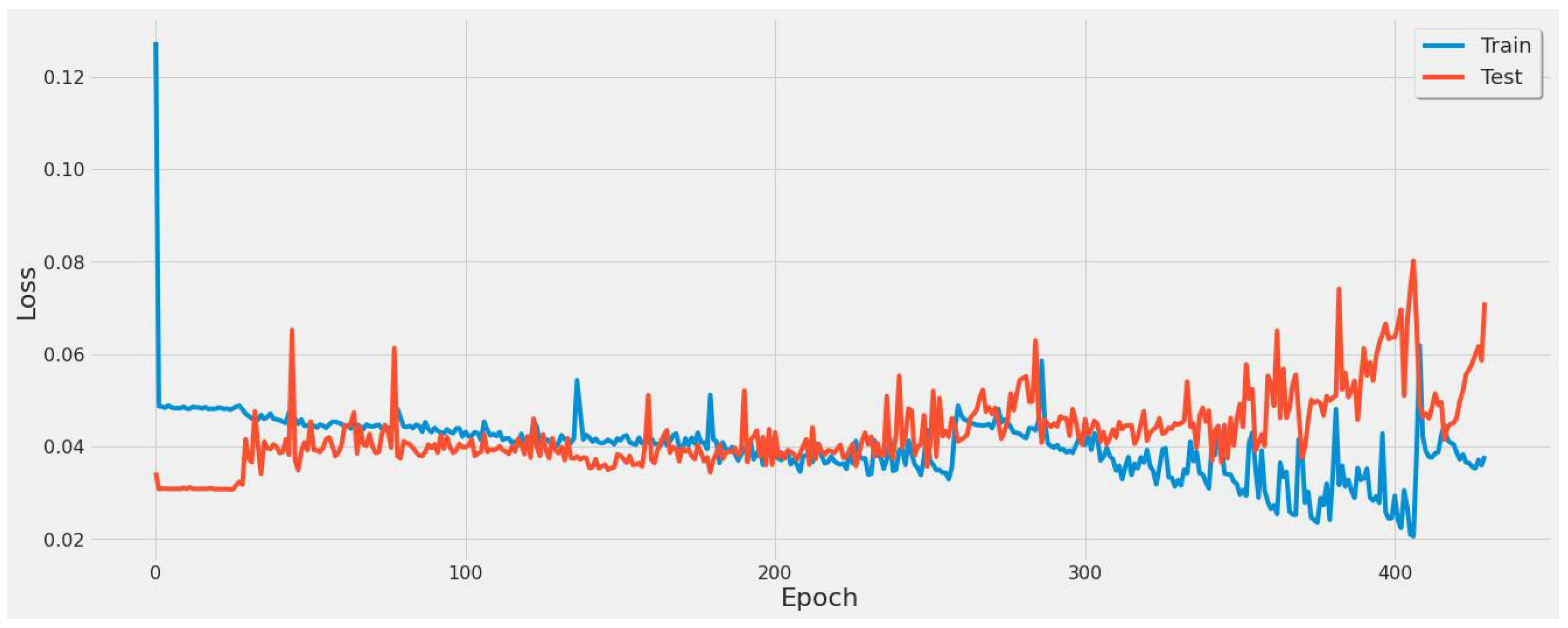
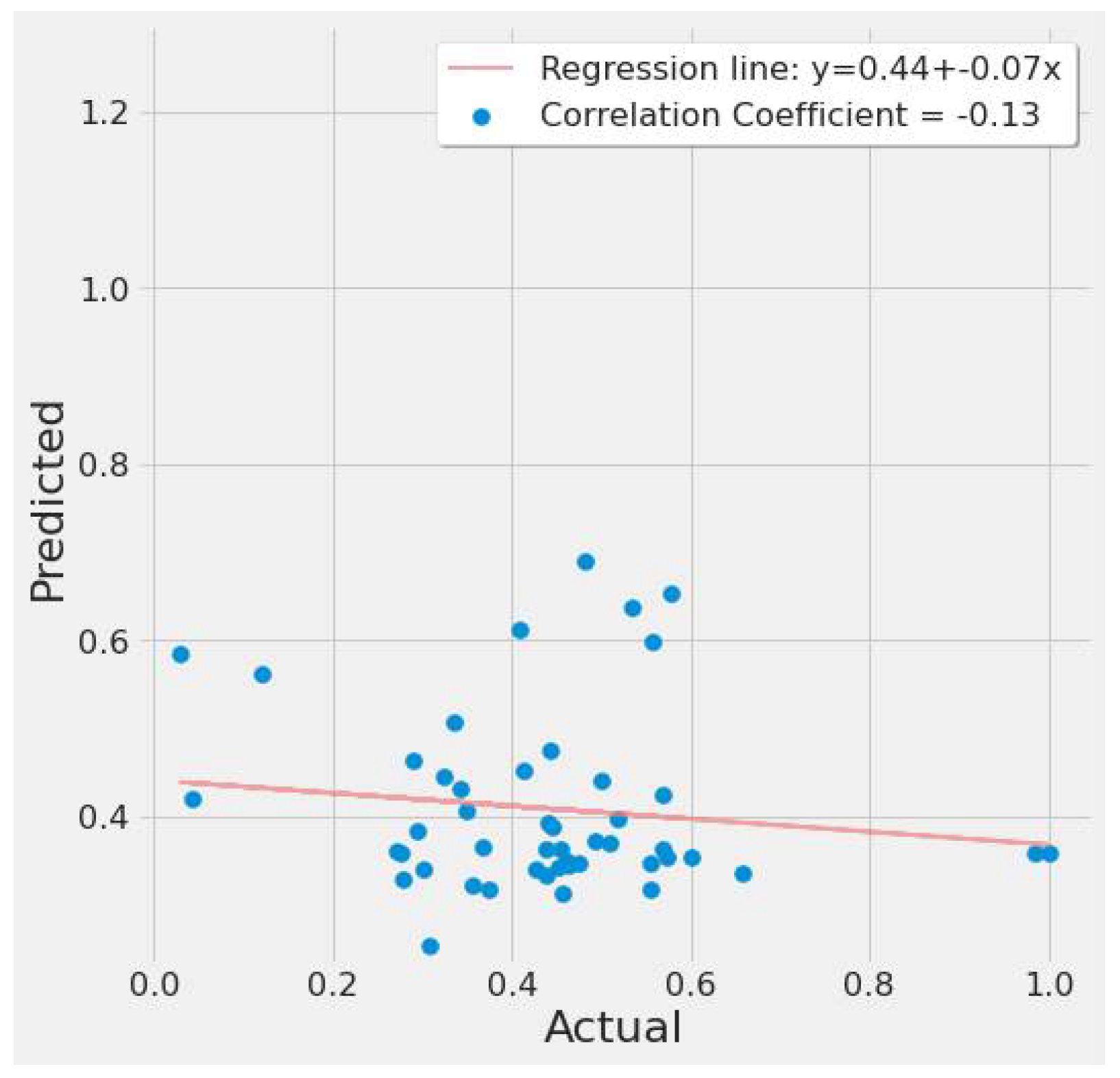
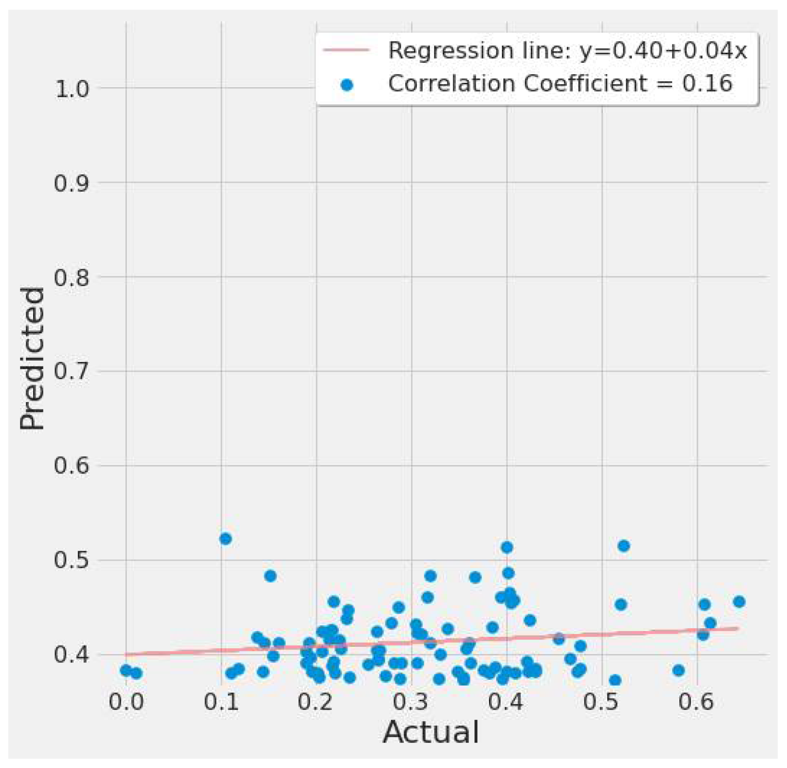
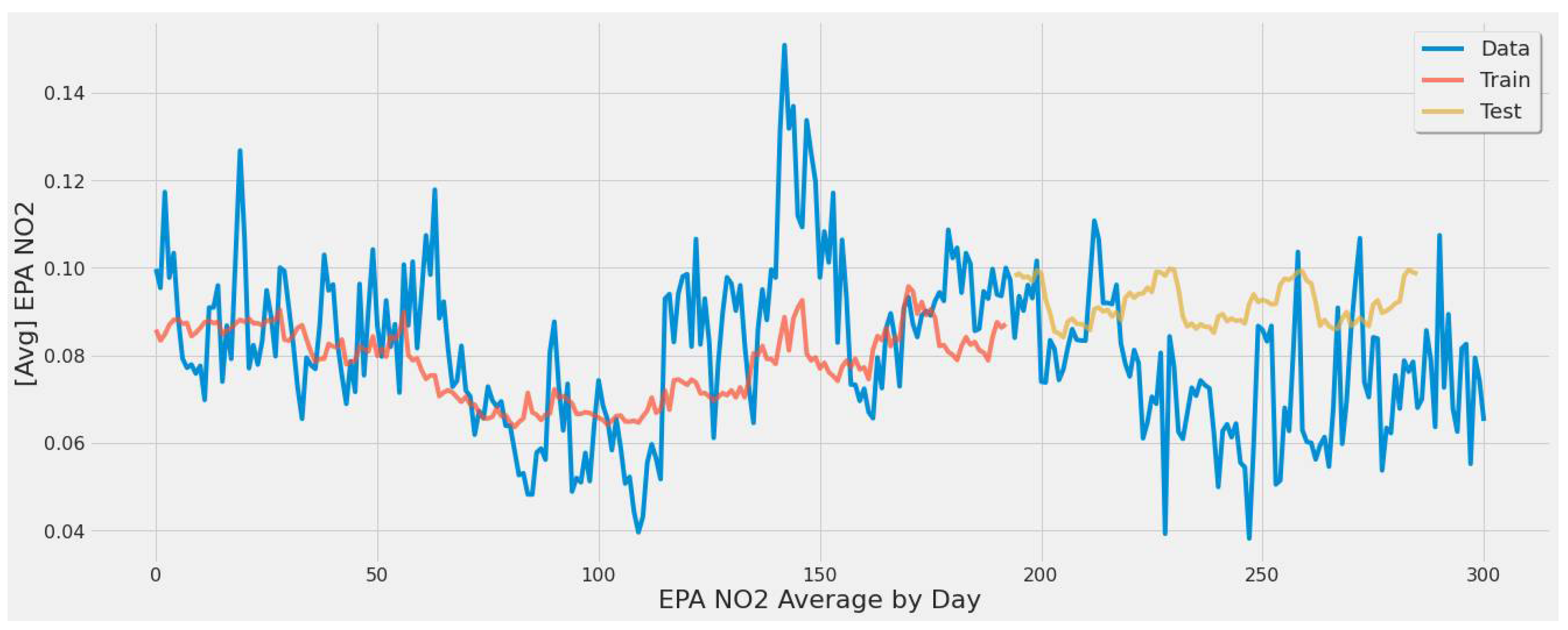
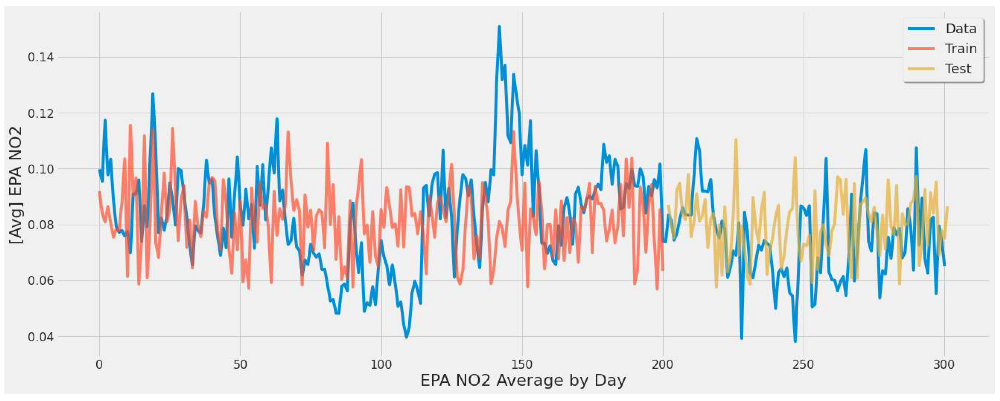
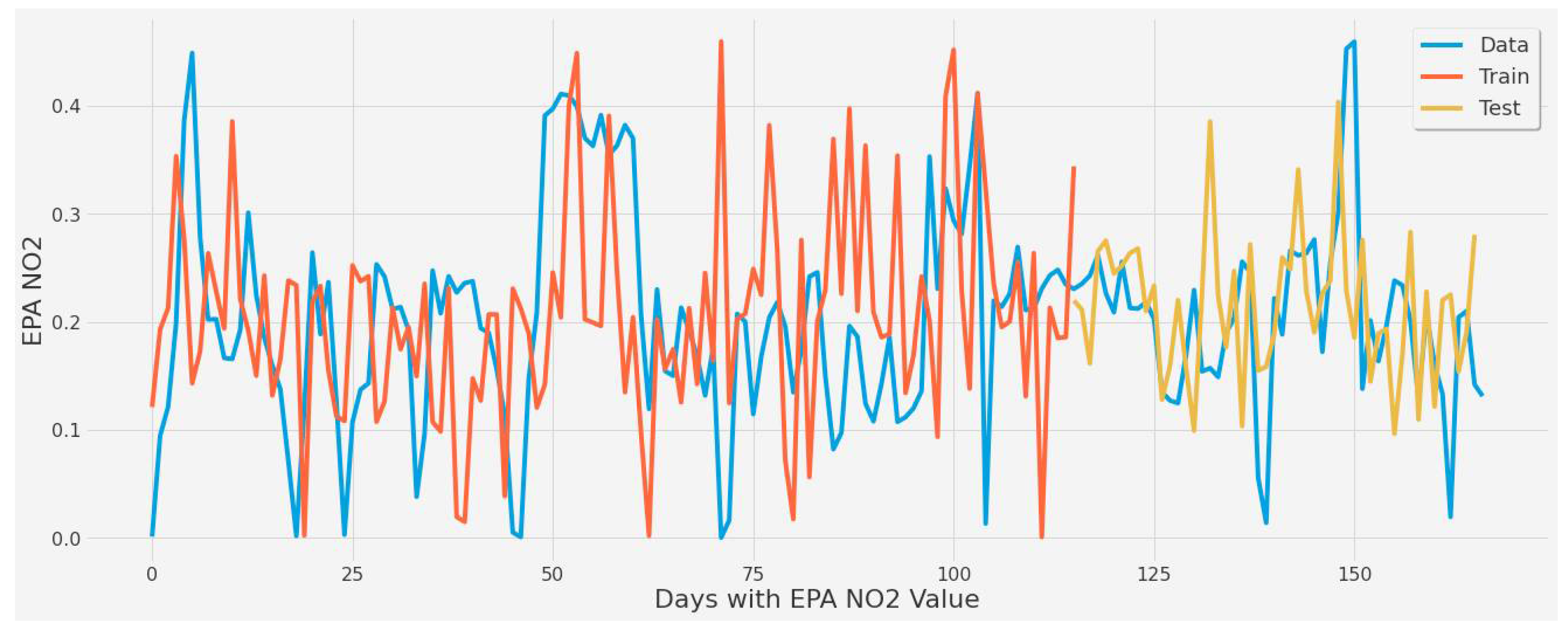
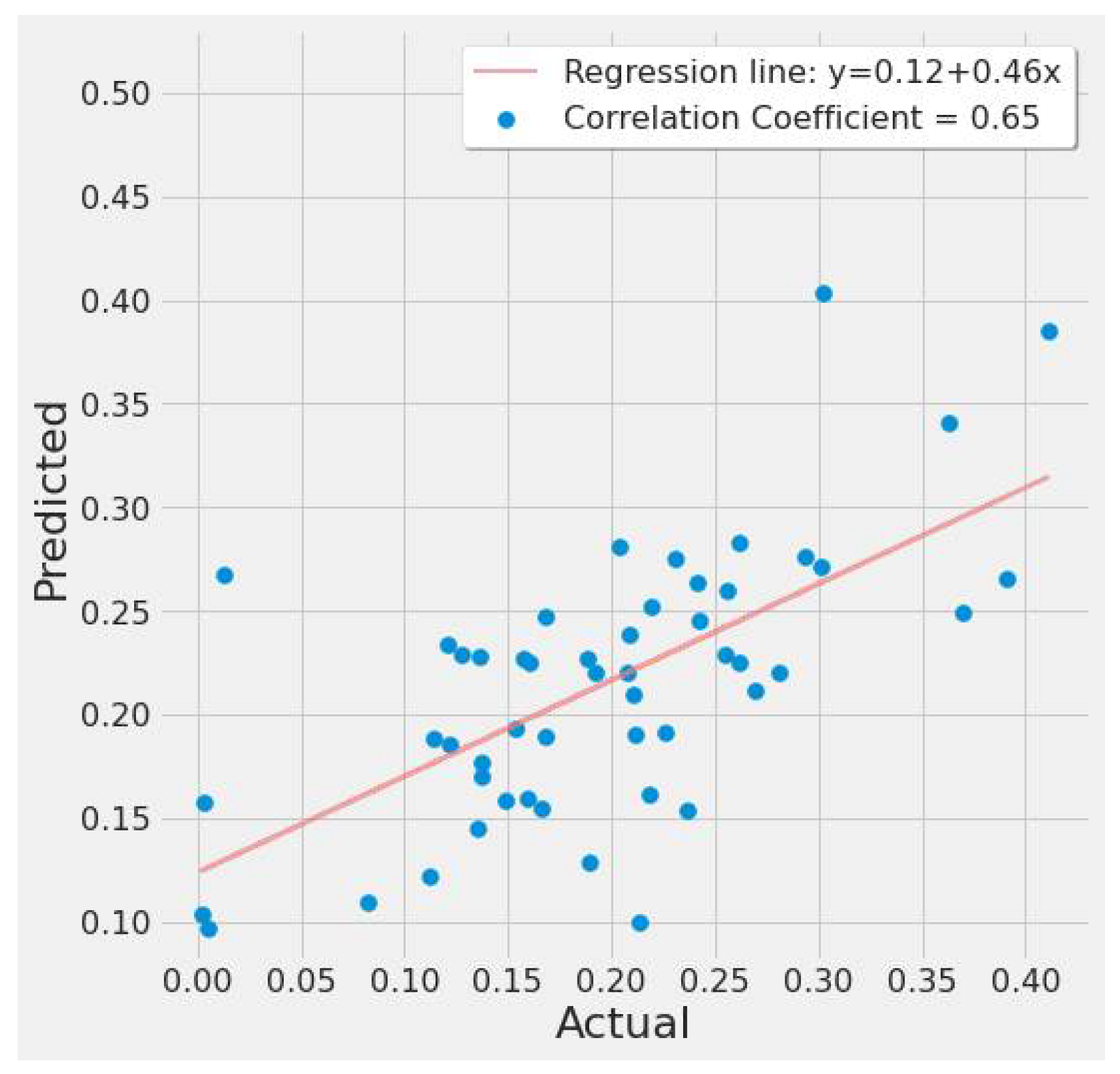
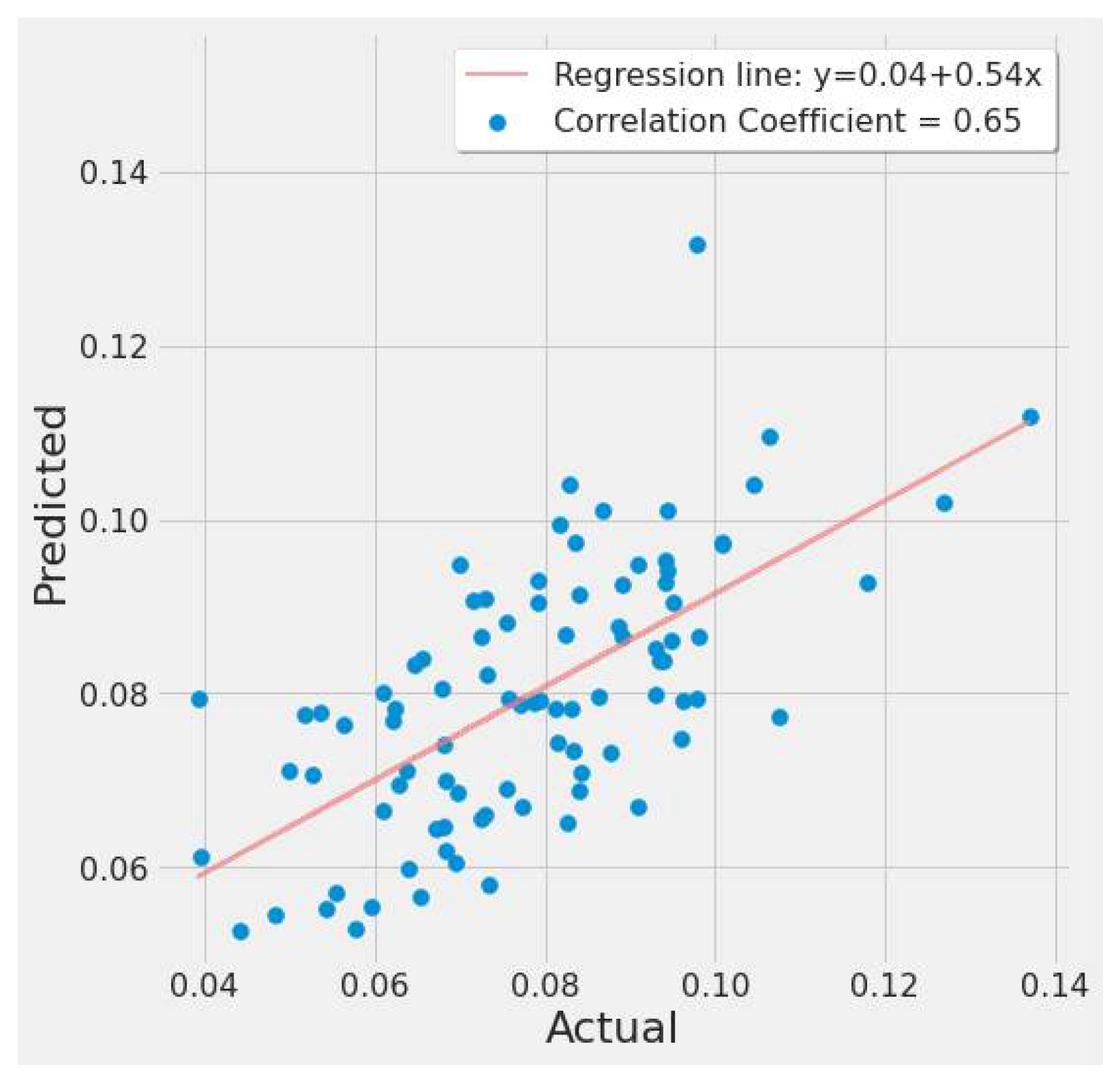
4.3.1. LSTM Results
4.3.2. SVR Results
4.3.3. RF Results
4.3.4. XGBoost Results
5. Discussion
5.1. Ability Assessment of ML and Remote Sensing on Predicting Single Source Emission
5.2. Spatiotemporal Pattern Discovery Using ML
5.3. Long-Term Operational Capability
5.4. Bias and Uncertainty
5.5. Study and ML limitations
- The data collected in this study mostly covered the essential sources for predicting NO2 emissions.
- More data volume for all data sources would have enhanced performance. The data collected was just for the year 2019, and it would have been beneficial to increase the sample size for all datasets.
- Sensor calibration and validation are integral for reliable remote sensing and proper quality of the derived variables/data. This study has ensured extraction of validated and filtered data to retrieve higher quality images of remotely sensed data. These processes are essential for better predictive modeling and, if lacking, can provide incorrect results.
- Passive remote sensing techniques (such as TROPOMI) record solar radiation reflected and emitted from Earth which can be sensitive to weather conditions, lowering their accuracy.
- The ML models and their predictive ability are the second main area of limitation.
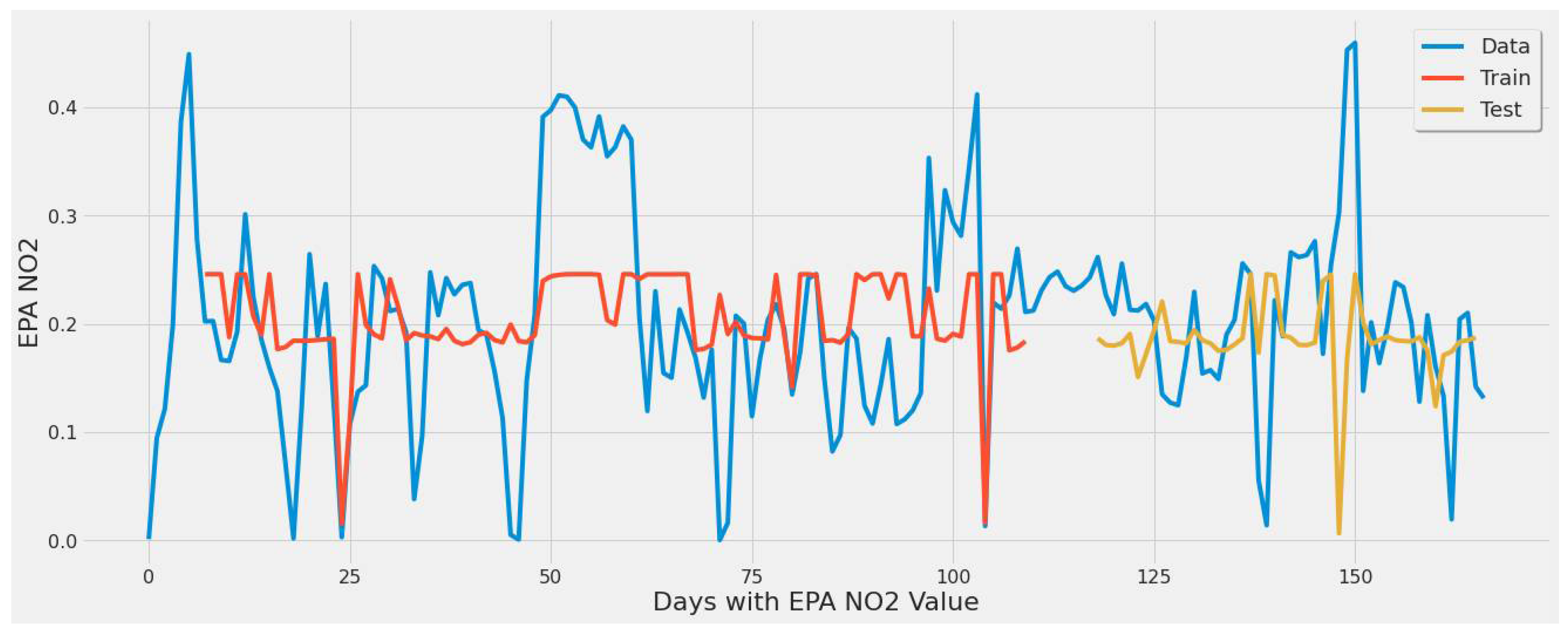
- For our first experimental scenario, the LSTM model captured extreme values well. However, it lacked low error rate results and had weak predictive ability, similar to our early testing models.
- The inclusion of a different LSTM architecture was a response to the unsatisfactory results of the original LSTM model tested, and the stacked architecture improved the results for the most part, but not significantly.
- The nonlinear nature of the data, along with the time series element, has traditionally been a complex problem to solve due primarily to random outcomes. The study’s main goal was to take a sample of results from multiple machine learning algorithms to draw conclusions and show that estimating NO2 emissions for power plants using remote sensing data was feasible.
- The study’s experiments were rigorously conducted and validated, but they were ultimately constrained by the volume of data and the predictive performance of our models.
- Additional data sources correlated with NO2 emissions and better remote sensing resolution could considerably improve the results in the future.
6. Conclusions and Future Work
Author Contributions
Funding
Acknowledgments
Conflicts of Interest
References
- Nitrogen Oxides (NOx), Why and How They Are Controlled.57. Available online: https://www3.epa.gov/ttn/catc/dir1/fnoxdoc.pdf (accessed on 15 December 2021).
- Srivastava, R.K.; Hall, R.E.; Khan, S.; Culligan, K.; Lani, B.W. Nitrogen Oxides Emission Control Options for Coal-Fired Electric Utility Boilers. J. Air Waste Manag. Assoc. 2005, 55, 1367–1388. [Google Scholar] [CrossRef] [PubMed] [Green Version]
- US EPA, O. Cleaner Power Plants. Available online: https://www.epa.gov/mats/cleaner-power-plants (accessed on 15 December 2021).
- Geostationary Satellite Constellation for Observing Global Air Quality: Geophysical Validation Needs. Available online: https://ceos.org/document_management/Publications/Publications-and-Key-Documents/Atmosphere/GEO_AQ_Constellation_Geophysical_Validation_Needs_1.1_2Oct2019.pdf (accessed on 15 December 2021).
- Beirle, S.; Borger, C.; Dörner, S.; Eskes, H.; Kumar, V.; de Laat, A.; Wagner, T. Catalog of NOx Emissions from Point Sources as Derived from the Divergence of the NO2 Flux for TROPOMI. Earth Syst. Sci. Data 2021, 13, 2995–3012. [Google Scholar] [CrossRef]
- Van der A, R.J.; de Laat, A.T.J.; Ding, J.; Eskes, H.J. Connecting the Dots: NOx Emissions along a West Siberian Natural Gas Pipeline. npj Clim. Atmos. Sci. 2020, 3, 1–7. [Google Scholar] [CrossRef] [Green Version]
- Hedley, J.; Russell, B.; Randolph, K.; Dierssen, H. A Physics-Based Method for the Remote Sensing of Seagrasses. Remote Sens. Environ. 2016, 174, 134–147. [Google Scholar] [CrossRef]
- Crosman, E. Meteorological Drivers of Permian Basin Methane Anomalies Derived from TROPOMI. Remote Sens. 2021, 13, 896. [Google Scholar] [CrossRef]
- Lorente, A.; Boersma, K.F.; Eskes, H.J.; Veefkind, J.P.; van Geffen, J.H.G.M.; de Zeeuw, M.B.; Denier van der Gon, H.A.C.; Beirle, S.; Krol, M.C. Quantification of Nitrogen Oxides Emissions from Build-up of Pollution over Paris with TROPOMI. Sci. Rep. 2019, 9, 20033. [Google Scholar] [CrossRef]
- Beirle, S.; Borger, C.; Dörner, S.; Li, A.; Hu, Z.; Liu, F.; Wang, Y.; Wagner, T. Pinpointing Nitrogen Oxide Emissions from Space. Sci. Adv. 2019, 5, eaax9800. [Google Scholar] [CrossRef] [Green Version]
- Ialongo, I.; Virta, H.; Eskes, H.; Hovila, J.; Douros, J. Comparison of TROPOMI/Sentinel-5 Precursor NO2 Observations with Ground-Based Measurements in Helsinki. Atmos. Meas. Tech. 2020, 13, 205–218. [Google Scholar] [CrossRef] [Green Version]
- Yu, M.; Liu, Q. Deep Learning-Based Downscaling of Tropospheric Nitrogen Dioxide Using Ground-Level and Satellite Ob-servations. Sci. Total Environ. 2021, 773, 145145. [Google Scholar] [CrossRef]
- Yang, G.; Wang, Y.; Li, X. Prediction of the NOx Emissions from Thermal Power Plant Using Long-Short Term Memory Neural Network. Energy 2020, 192, 116597. [Google Scholar] [CrossRef]
- Karim, R.; Rafi, T.H. An Automated LSTM-Based Air Pollutant Concentration Estimation of Dhaka City, Bangladesh. Int. J. Eng. Inf. Syst. 2020, 4, 88–101. [Google Scholar]
- Kristiani, E.; Kuo, T.-Y.; Yang, C.-T.; Pai, K.-C.; Huang, C.-Y.; Nguyen, K.L.P. PM2.5 Forecasting Model Using a Combination of Deep Learning and Statistical Feature Selection. IEEE Access 2021, 9, 68573–68582. [Google Scholar] [CrossRef]
- Abimannan, S.; Chang, Y.-S.; Lin, C.-Y. Air Pollution Forecasting Using LSTM-Multivariate Regression Model. In Proceedings of the Internet of Vehicles, Technologies and Services Toward Smart Cities, Kaohsiung, Taiwan, 18–21 November 2019; Hsu, C.-H., Kallel, S., Lan, K.-C., Zheng, Z., Eds.; Springer International Publishing: Cham, Switzerland, 2020; pp. 318–326. [Google Scholar]
- Georgoulias, A.K.; Boersma, K.F.; van Vliet, J.; Zhang, X.; Zanis, P.; Laat, J. Detection of NO2 Pollution Plumes from Individual Ships with the TROPOMI/S5P Satellite Sensor. Environ. Res. Lett. 2020, 15, 124037. [Google Scholar] [CrossRef]
- Si, M.; Du, K. Development of a Predictive Emissions Model Using a Gradient Boosting Machine Learning Method. Environ. Technol. Innov. 2020, 20, 101028. [Google Scholar] [CrossRef]
- Zhan, Y.; Luo, Y.; Deng, X.; Zhang, K.; Zhang, M.; Grieneisen, M.L.; Di, B. Satellite-Based Estimates of Daily NO2 Exposure in China Using Hybrid Random Forest and Spatiotemporal Kriging Model. Environ. Sci. Technol. 2018, 52, 4180–4189. [Google Scholar] [CrossRef]
- Chen, T.-H.; Hsu, Y.-C.; Zeng, Y.-T.; Candice Lung, S.-C.; Su, H.-J.; Chao, H.J.; Wu, C.-D. A Hybrid Kriging/Land-Use Regres-sion Model with Asian Culture-Specific Sources to Assess NO2 Spatial-Temporal Variations. Environ. Pollut. 2020, 259, 113875. [Google Scholar] [CrossRef] [PubMed]
- Novotny, E.V.; Bechle, M.J.; Millet, D.B.; Marshall, J.D. National Satellite-Based Land-Use Regression: NO2 in the United States. Environ. Sci. Technol. 2011, 45, 4407–4414. [Google Scholar] [CrossRef] [PubMed]
- Wong, P.-Y.; Su, H.-J.; Lee, H.-Y.; Chen, Y.-C.; Hsiao, Y.-P.; Huang, J.-W.; Teo, T.-A.; Wu, C.-D.; Spengler, J.D. Using Land-Use Machine Learning Models to Estimate Daily NO2 Concentration Variations in Taiwan. J. Clean. Prod. 2021, 317, 128411. [Google Scholar] [CrossRef]
- El Khoury, E.; Ibrahim, E.; Ghanimeh, S. A Look at the Relationship Between Tropospheric Nitrogen Dioxide and Aerosol Optical Thickness Over Lebanon Using Spaceborne Data of the Copernicus Programme. In Proceedings of the 2019 Fourth International Conference on Advances in Computational Tools for Engineering Applications (ACTEA), Beirut, Lebanon, 3–5 July 2019; pp. 1–6. [Google Scholar]
- Lin, C.-A.; Chen, Y.-C.; Liu, C.-Y.; Chen, W.-T.; Seinfeld, J.H.; Chou, C.C.-K. Satellite-Derived Correlation of SO2, NO2, and Aerosol Optical Depth with Meteorological Conditions over East Asia from 2005 to 2015. Remote Sens. 2019, 11, 1738. [Google Scholar] [CrossRef] [Green Version]
- Superczynski, S.D.; Kondragunta, S.; Lyapustin, A.I. Evaluation of the Multi-Angle Implementation of Atmospheric Correc-tion (MAIAC) Aerosol Algorithm through Intercomparison with VIIRS Aerosol Products and AERONET. J. Geophys. Res. Atmos. 2017, 122, 3005–3022. [Google Scholar] [CrossRef] [Green Version]
- Zhao, X.; Griffin, D.; Fioletov, V.; McLinden, C.; Cede, A.; Tiefengraber, M.; Müller, M.; Bognar, K.; Strong, K.; Boersma, F.; et al. Assessment of the Quality of TROPOMI High-Spatial-Resolution NO2 Data Products in the Greater Toronto Area. Atmos. Meas. Tech. 2020, 13, 2131–2159. [Google Scholar] [CrossRef]
- Verhoelst, T.; Compernolle, S.; Pinardi, G.; Lambert, J.-C.; Eskes, H.J.; Eichmann, K.-U.; Fjæraa, A.M.; Granville, J.; Niemeijer, S.; Cede, A.; et al. Ground-Based Validation of the Copernicus Sentinel-5P TROPOMI NO2 Measurements with the NDACC ZSL-DOAS, MAX-DOAS and Pandonia Global Networks. Atmos. Meas. Tech. 2021, 14, 481–510. [Google Scholar] [CrossRef]
- Wang, C.; Wang, T.; Wang, P.; Rakitin, V. Comparison and Validation of TROPOMI and OMI NO2 Observations over China. Atmosphere 2020, 11, 636. [Google Scholar] [CrossRef]
- The Aura Mission. Available online: https://aura.gsfc.nasa.gov/omi.html (accessed on 14 December 2021).
- Khatibi, A.; Krauter, S. Validation and Performance of Satellite Meteorological Dataset MERRA-2 for Solar and Wind Applications. Energies 2021, 14, 882. [Google Scholar] [CrossRef]
- Merrill, R. Procedure 1. Quality Assurance Requirements for Gas Continuous Emission Monitoring Systems Used for Compliance Determination; EPA: Washington, DC, USA, 2020; 9p.
- US EPA, O. National Emissions Inventory (NEI). Available online: https://www.epa.gov/air-emissions-inventories/national-emissions-inventory-nei (accessed on 10 December 2021).
- Sun, Z.; Sandoval, L.; Crystal-Ornelas, R.; Mousavi, S.M.; Wang, J.; Lin, C.; Cristea, N.; Tong, D.; Carande, W.H.; Ma, X.; et al. A Review of Earth Artificial Intelligence. Comput. Geosci. 2022, 159, 105034. [Google Scholar] [CrossRef]


| EPA_NO2/100,000 | TROPOMI*1000 | Wind (Daily) | Temp (Daily) | Precip (Daily) | Cloud Fraction (Daily) | day of year | day of week | day of month | Optical_Depth_047 | |
|---|---|---|---|---|---|---|---|---|---|---|
| Count | 167 | 167 | 167 | 167 | 167 | 167 | 167 | 167 | 167 | 167 |
| Mean | 0.202 | 0.073 | −0.002283 | 292.429054 | 0.000047 | 0.481267 | 190.892 | 3.023 | 15.640 | 83.401 |
| Std | 0.095 | 0.017 | 0.066753 | 8.760018 | 0.000109 | 0.275749 | 98.860 | 1.987 | 9.297 | 116.695 |
| Min | 0.000180 | 0.038 | −0.248446 | 273.780730 | 0 | 0.000238 | 16.000 | 0 | 1 | 0 |
| Max | 0.459 | 0.127 | 0.340735 | 304.310400 | 0.000660 | 0.957011 | 339 | 6 | 31 | 529 |
| EPA_NO2/100,000 | TROPOMI*1000 | day of year | day of week | day of month | |
|---|---|---|---|---|---|
| Count | 8887 | 8887 | 8887 | 8887 | 8887 |
| Mean | 0.080 | 0.103 | 174.562 | 2.938 | 15.730 |
| Std | 0.116 | 0.076 | 109.798 | 1.986 | 8.682 |
| Min | 0 | 0.0002 | 1 | 0 | 1 |
| Max | 0.908 | 1.904 | 365 | 6 | 31 |
| Models | Mean Average Error | Mean Square Error | Root Mean Square Error | Residual Standard Error | Error Rate |
|---|---|---|---|---|---|
| Linear Regression | 0.08101 | 0.0111 | 0.1057 | 0.0143 | 0.5486 |
| Random Forest | 0.0702 | 0.008 | 0.0925 | 0.0125 | 0.4797 |
| Multilayer Perceptron | 0.0716 | 0.009 | 0.0965 | 0.0131 | 0.5005 |
| Voting Ensemble | 0.0726 | 0.0088 | 0.0938 | 0.0127 | 0.4867 |
| Number | Experiments | Mean Average Error | Mean Square Error | Root Mean Square Error | Residual Standard Error | Error Rate |
|---|---|---|---|---|---|---|
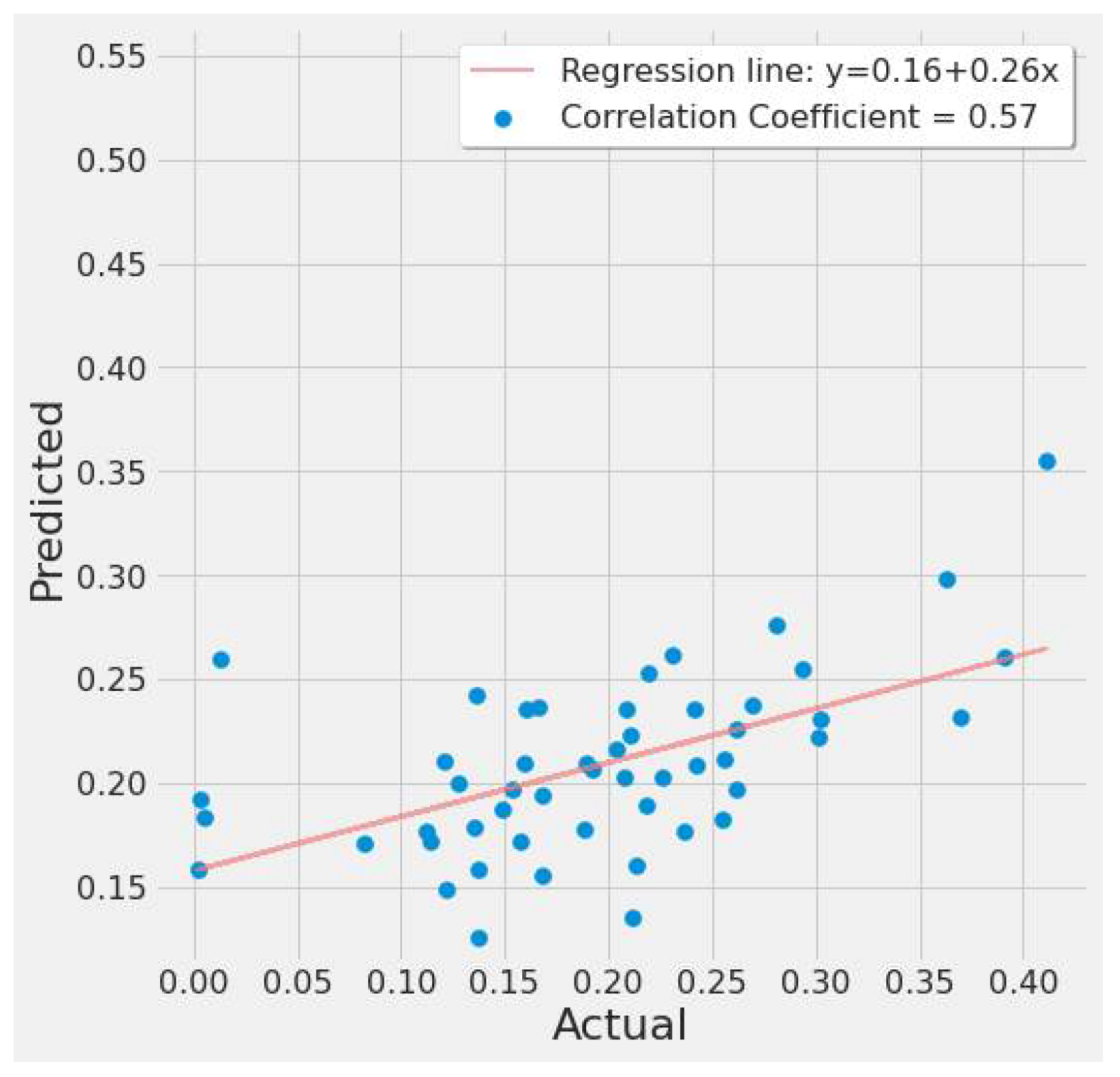
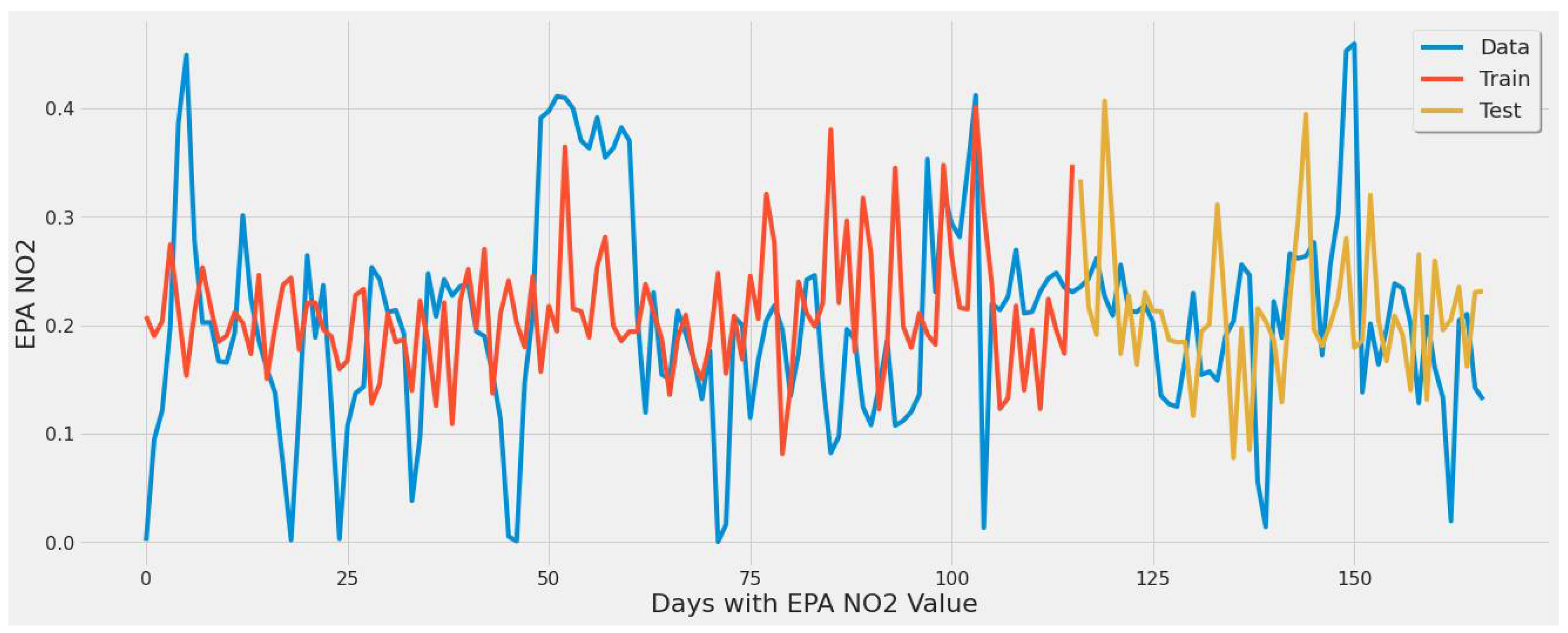
| 1 | Stacked LSTM [Alabama Plant TROPOMI input only] Epochs 250 | 0.1414 | 0.0424 | 0.2060 | 0.0303 | 0.4685 |
| 2 | Stacked LSTM [Alabama Plant TROPOMI input only] Epochs 380 | 0.1546 | 0.0443 | 0.2106 | 0.0310 | 0.4788 |
| 3 | Stacked LSTM [Alabama Plant TROPOMI input only] Epochs 430 | 0.1535 | 0.0491 | 0.2217 | 0.0326 | 0.5040 |
| 4 | Stacked LSTM [Alabama Plant TROPOMI/MERRA-2 Monthly/Date inputs] Epochs 250 | 0.1332 | 0.0375 | 0.1938 | 0.0285 | 0.4406 |
| 5 | Stacked LSTM [Alabama Plant TROPOMI/MERRA-2 Monthly /Date inputs] Epochs 380 | 0.1316 | 0.0371 | 0.1927 | 0.0284 | 0.4383 |
| 6 | Stacked LSTM [Alabama Plant TROPOMI/MERRA-2 Monthly /Date inputs] Epochs 430 | 0.1450 | 0.0420 | 0.2051 | 0.0302 | 0.4663 |
| 7 | Stacked LSTM [Alabama Plant TROPOMI/MERRA-2 Daily/Date inputs] Epochs 250 | 0.1587 | 0.0468 | 0.2164 | 0.0319 | 0.4921 |
| 8 | Stacked LSTM [Alabama Plant TROPOMI/MERRA-2 Daily/Date inputs] Epochs 380 | 0.1415 | 0.0398 | 0.1997 | 0.0294 | 0.4541 |
| 9 | Stacked LSTM [Alabama Plant TROPOMI/MERRA-2 Daily/Date inputs] Epochs 430 | 0.1627 | 0.0485 | 0.2203 | 0.0324 | 0.5009 |
| 10 | Stacked LSTM [Alabama Plant MERRA-2 daily input only] Epochs 250 | 0.1300 | 0.0340 | 0.1846 | 0.0272 | 0.4197 |
| 11 | Stacked LSTM [Alabama Plant MERRA-2 daily input only] Epochs 380 | 0.1334 | 0.0356 | 0.1888 | 0.0278 | 0.4293 |
| 12 | Stacked LSTM [Alabama Plant MERRA-2 daily input only] Epochs 430 | 0.1396 | 0.0377 | 0.1942 | 0.0286 | 0.4415 |
| 13 | Stacked LSTM [Alabama Plant TROPOMI/MERRA-2 Weekly/Date inputs] Epochs 250 | 0.1359 | 0.0355 | 0.1884 | 0.0277 | 0.4284 |
| 14 | Stacked LSTM [Alabama Plant TROPOMI/MERRA-2 Weekly/Date inputs] Epochs 380 | 0.1491 | 0.0438 | 0.2094 | 0.0308 | 0.4761 |
| 15 | Stacked LSTM [Alabama Plant TROPOMI/MERRA-2 Weekly/Date inputs] Epochs 430 | 0.1401 | 0.0381 | 0.1952 | 0.0287 | 0.4438 |
| 16 | Stacked LSTM [Alabama Plant TROPOMI/MERRA-2 Monthly /MCD19A2/Date inputs] Epochs 250 | 0.1485 | 0.0439 | 0.2096 | 0.0309 | 0.4766 |
| 17 | Stacked LSTM [Alabama Plant TROPOMI/MERRA-2 Monthly /MCD19A2/Date inputs] Epochs 380 | 0.1260 | 0.0348 | 0.1865 | 0.0275 | 0.4241 |
| 18 | Stacked LSTM [Alabama Plant TROPOMI/MERRA-2 Monthly /MCD19A2/Date inputs] Epochs 430 | 0.1615 | 0.0506 | 0.2250 | 0.0331 | 0.5116 |
| 19 | Stacked LSTM [Alabama Plant TROPOMI/MERRA-2 Daily/MCD19A2/Date inputs] Epochs 250 | 0.1581 | 0.0453 | 0.2128 | 0.0313 | 0.4839 |
| 20 | Stacked LSTM [Alabama Plant TROPOMI/MERRA-2 Daily/MCD19A2/Date inputs] Epochs 380 | 0.1219 | 0.0308 | 0.1757 | 0.0259 | 0.3995 |
| 21 | Stacked LSTM [Alabama Plant TROPOMI/MERRA-2 Daily/MCD19A2/Date inputs] Epochs 430 | 0.1558 | 0.0456 | 0.2137 | 0.0315 | 0.4859 |
| 22 | Stacked LSTM [Alabama Plant TROPOMI/MERRA-2 Weekly/MCD19A2/Date inputs] Epochs 250 | 0.1499 | 0.0426 | 0.2066 | 0.0304 | 0.4697 |
| 23 | Stacked LSTM [Alabama Plant TROPOMI/MERRA-2 Weekly/MCD19A2/Date inputs] Epochs 380 | 0.1607 | 0.0457 | 0.2138 | 0.0315 | 0.4863 |
| 24 | Stacked LSTM [Alabama Plant TROPOMI/MERRA-2 Weekly/MCD19A2/Date inputs] Epochs 430 | 0.1653 | 0.0496 | 0.2227 | 0.0328 | 0.5065 |
| Index | Actual EPA NO2 | Predicted EPA NO2 |
|---|---|---|
| 0 | 0.569089 | 0.428293 |
| 1 | 0.492650 | 0.513841 |
| 2 | 0.454344 | 0.385182 |
| 3 | 0.556001 | 0.389160 |
| 4 | 0.463098 | 0.514868 |
| 5 | 0.461661 | 0.384444 |
| 6 | 0.474771 | 0.286175 |
| …. | …. | |
| 41 | 0.452296 | 0.376052 |
| 42 | 0.349115 | 0.287791 |
| 43 | 0.289771 | 0.366804 |
| 44 | 0.041835 | 0.377947 |
| 45 | 0.444348 | 0.398745 |
| 46 | 0.456870 | 0.391060 |
| Number | Experiments | Mean Average Error | Mean Square Error | Root Mean Square Error | Residual Standard Error | Error Rate |
|---|---|---|---|---|---|---|
| 1 | Stacked LSTM [All 289 Power Plants Average TROPOMI/Date inputs] 380 epochs | 0.1604 | 0.0366 | 0.1914 | 0.0201 | 0.6098 |
| 2 | Stacked LSTM [All 289 Power Plants Average TROPOMI/Date inputs] 430 epochs | 0.1667 | 0.0400 | 0.2000 | 0.0210 | 0.6371 |
| 3 | Stacked LSTM [All 289 Power Plants Average TROPOMI/Date inputs] 800 epochs | 0.1465 | 0.0306 | 0.1751 | 0.0184 | 0.5579 |
| Results | Hyperparameters | ||||||||
|---|---|---|---|---|---|---|---|---|---|
| Number | Experiments | Mean Average Error | Mean Square Error | Root Mean Square Error | Residual Standard Error | Error Rate | Coefficient (Gamma) | Regularization Parameter (C) | Epsilon Value |
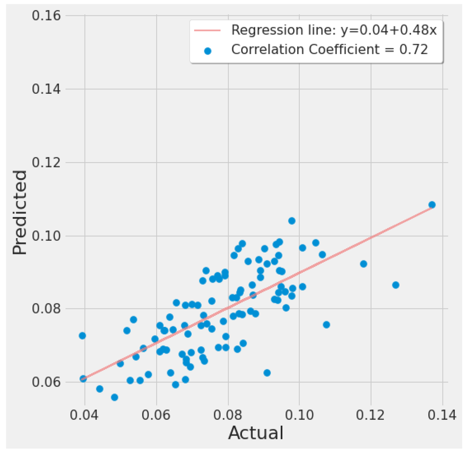
| 1 | SVR GridSearch Best Params [Alabama Plant TROPOMI input only] | 0.0686 | 0.0080 | 0.0896 | 0.0128 | 0.4576 | 0.1 | 10,000 | 0.05 |
| 2 | SVR GridSearch Best Params [Alabama Plant TROPOMI/MERRA-2/Date inputs] | 0.0492 | 0.0043 | 0.0658 | 0.0094 | 0.3360 | 0.001 | 1 | 0.01 |
| 3 | SVR GridSearch Best Params [Alabama Plant TROPOMI/MERRA-2 Daily/Date inputs] | 0.0483 | 0.0040 | 0.0634 | 0.0090 | 0.3240 | 0.001 | 1 | 0.05 |
| 4 | SVR GridSearch Best Params [Alabama Plant TROPOMI/MERRA-2 Daily/MCD19A2/Date inputs] | 0.0550 | 0.0057 | 0.0758 | 0.0108 | 0.3874 | 0.001 | 0.1 | 0.01 |
| 5 | SVR GridSearch Best Params [Alabama Plant MERRA-2 Daily/Date inputs] | 0.0572 | 0.0054 | 0.0739 | 0.0105 | 0.3776 | 0.01 | 1 | 0.05 |
| 6 | SVR GridSearch Best Params [Alabama Plant TROPOMI/MERRA-2 Weekly/Date inputs] | 0.0555 | 0.0056 | 0.0750 | 0.0107 | 0.3832 | 0.01 | 0.1 | 0.01 |
| 7 | SVR GridSearch Best Params [Alabama Plant TROPOMI/MERRA-2 Weekly/MCD19A2/Date inputs] | 0.0572 | 0.0062 | 0.0792 | 0.0113 | 0.4047 | 0.01 | 0.1 | 0.0001 |
| 8 | SVR GridSearch Best Params [Alabama Plant TROPOMI/MERRA-2/MCD19A2/Date inputs] | 0.0537 | 0.0055 | 0.0745 | 0.0106 | 0.3804 | 0.01 | 0.1 | 0.001 |
| 9 | SVR GridSearch Best Params [All 289 Power Plants TROPOMI input only] | 0.01402 | 0.0003 | 0.0177 | 0.0017 | 0.2264 | 0.0001 | 1000 | 0.01 |
| 10 | SVR GridSearch Best Params [All 289 Power Plants TROPOMI/Date inputs] | 0.0095 | 0.0001 | 0.0121 | 0.0012 | 0.1552 | 0.01 | 0.1 | 0.005 |
| Results | Hyperparameters | ||||||||
|---|---|---|---|---|---|---|---|---|---|
| Number | Experiments | Mean Average Error | Mean Square Error | Root Mean Square Error | Residual Standard Error | Error Rate | Trees | Max Depth | Min Samples |
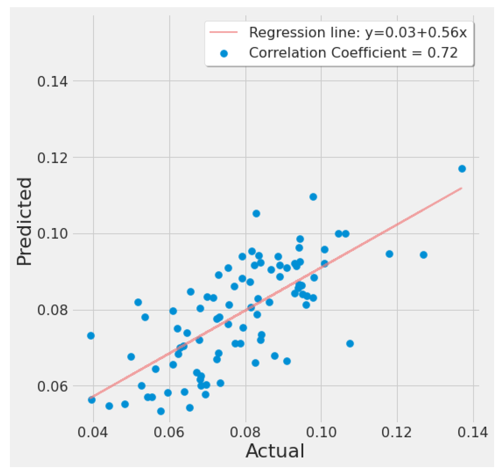
| 1 | RF [Alabama Power Plant TROPOMI input only] | 0.0795 | 0.0110 | 0.1050 | 0.0150 | 0.5361 | 1000 | 20 | 2 |
| 2 | RF [Alabama Power Plant TROPOMI/MERRA-2/Date inputs] | 0.0525 | 0.0050 | 0.0711 | 0.0101 | 0.3632 | 1000 | 15 | 2 |
| 3 | RF GridSearch Best Params [Alabama Power Plant TROPOMI input only] | 0.0484 | 0.0044 | 0.0666 | 0.0095 | 0.3401 | 1000 | 20 | 2 |
| 4 | RF GridSearch Best Params [Alabama Power Plant TROPOMI/MERRA-2 Monthly/Date inputs] | 0.0488 | 0.0044 | 0.0667 | 0.0095 | 0.3410 | 1000 | 110 | 2 |
| 5 | RF GridSearch Best Params [Alabama Power Plant TROPOMI/MERRA-2 Monthly/MCD19A2/Date inputs] | 0.0509 | 0.0049 | 0.0705 | 0.0100 | 0.3604 | 1000 | 70 | 10 |
| 6 | RF GridSearch Best Params [Alabama Power Plant TROPOMI/MERRA-2 Daily/Date inputs] | 0.0582 | 0.006 | 0.077 | 0.011 | 0.396 | 800 | 100 | 2 |
| 7 | RF GridSearch Best Params [Alabama Power Plant TROPOMI/MERRA-2 Daily/MCD19A2/Date inputs] | 0.059 | 0.006 | 0.078 | 0.011 | 0.399 | 800 | 30 | 5 |
| 8 | RF GridSearch Best Params [Alabama Power Plant MERRA-2 Daily/Date inputs] | 0.058 | 0.006 | 0.077 | 0.011 | 0.396 | 800 | 80 | 5 |
| 9 | RF GridSearch Best Params [Alabama Power Plant TROPOMI/MERRA-2 Weekly/Date inputs] | 0.064 | 0.007 | 0.085 | 0.012 | 0.436 | 800 | 10 | 2 |
| 10 | RF GridSearch Best Params [Alabama Power Plant TROPOMI/MERRA-2 Weekly/MCD19A2/Date inputs] | 0.064 | 0.007 | 0.085 | 0.012 | 0.438 | 800 | 90 | 2 |
| 11 | RF GridSearch Best Params [All 289 Power Plants Average TROPOMI only] | 0.0157 | 0.0003 | 0.0198 | 0.0021 | 0.2530 | 400 | 80 | 2 |
| 12 | RF GridSearch Best Params [All 289 Power Plants Average TROPOMI/Date inputs] | 0.0099 | 0.0001 | 0.0125 | 0.0013 | 0.1592 | 1800 | 80 | 2 |
| Number | Experiments | Mean Average Error | Mean Square Error | Root Mean Square Error | Residual Standard Error | Error Rate |
|---|---|---|---|---|---|---|
| 1 | XGBoost [Alabama Plant TROPOMI input only] | 0.0933 | 0.0159 | 0.1262 | 0.0180 | 0.6445 |
| 2 | XGBoost [Alabama Plant TROPOMI/MERRA-2 Monthly/Date inputs] | 0.0542 | 0.0051 | 0.0718 | 0.0102 | 0.3669 |
| 3 | XGBoost [Alabama Plant TROPOMI/MERRA-2 Monthly /MCD19A2/Date inputs] | 0.0587 | 0.0060 | 0.0778 | 0.0111 | 0.3974 |
| 4 | XGBoost [Alabama Plant TROPOMI/MERRA-2 Daily/Date inputs] | 0.071 | 0.008 | 0.094 | 0.013 | 0.484 |
| 5 | XGBoost [Alabama Plant TROPOMI/MERRA-2 Daily/MCD19A2/Date inputs] | 0.0726 | 0.009 | 0.096 | 0.013 | 0.493 |
| 6 | XGBoost [Alabama Plant MERRA-2 Daily/Date inputs] | 0.071 | 0.008 | 0.093 | 0.013 | 0.479 |
| 7 | XGBoost [Alabama Plant TROPOMI/MERRA-2 Weekly/Date inputs] | 0.063 | 0.006 | 0.082 | 0.011 | 0.421 |
| 8 | XGBoost [Alabama Plant TROPOMI/MERRA-2 Weekly/MCD19A2/Date inputs] | 0.067 | 0.007 | 0.088 | 0.012 | 0.450 |
| 9 | XGBoost [All 289 Power Plants Average TROPOMI/Date inputs] | 0.0112 | 0.0001 | 0.0140 | 0.0014 | 0.1793 |
Publisher’s Note: MDPI stays neutral with regard to jurisdictional claims in published maps and institutional affiliations. |
© 2022 by the authors. Licensee MDPI, Basel, Switzerland. This article is an open access article distributed under the terms and conditions of the Creative Commons Attribution (CC BY) license (https://creativecommons.org/licenses/by/4.0/).
Share and Cite
Alnaim, A.; Sun, Z.; Tong, D. Evaluating Machine Learning and Remote Sensing in Monitoring NO2 Emission of Power Plants. Remote Sens. 2022, 14, 729. https://doi.org/10.3390/rs14030729
Alnaim A, Sun Z, Tong D. Evaluating Machine Learning and Remote Sensing in Monitoring NO2 Emission of Power Plants. Remote Sensing. 2022; 14(3):729. https://doi.org/10.3390/rs14030729
Chicago/Turabian StyleAlnaim, Ahmed, Ziheng Sun, and Daniel Tong. 2022. "Evaluating Machine Learning and Remote Sensing in Monitoring NO2 Emission of Power Plants" Remote Sensing 14, no. 3: 729. https://doi.org/10.3390/rs14030729
APA StyleAlnaim, A., Sun, Z., & Tong, D. (2022). Evaluating Machine Learning and Remote Sensing in Monitoring NO2 Emission of Power Plants. Remote Sensing, 14(3), 729. https://doi.org/10.3390/rs14030729