Article

Active Fire Mapping on Brazilian Pantanal Based on Deep Learning and CBERS 04A Imagery

1
Faculty of Engineering, Architecture and Urbanism and Geography, Federal University of Mato Grosso do Sul, Campo Grande 79070-900, Brazil
2
Laboratory of Atmospheric Sciences, Institute of Physics, Federal University of Mato Grosso do Sul, Campo Grande 79070-900, Brazil
3
Department of Forest Engineering, Santa Catarina State University, Lages 88520-000, Brazil
4
Departamento de Meteorologia, Universidade Federal do Rio de Janeiro, Rio de Janeiro 21941-916, Brazil
5
Faculty of Computer Science, Federal University of Mato Grosso do Sul, Campo Grande 79070-900, Brazil
*
Author to whom correspondence should be addressed.
Remote Sens. 2022, 14(3), 688; https://doi.org/10.3390/rs14030688
Submission received: 13 December 2021 / Revised: 16 January 2022 / Accepted: 21 January 2022 / Published: 31 January 2022

Abstract

:
Fire in Brazilian Pantanal represents a serious threat to biodiversity. The Brazilian National Institute of Spatial Research (INPE) has a program named Queimadas, which estimated from January 2020 to October 2020, a burned area in Pantanal of approximately 40,606 km 2 . This program also provides daily data of active fire (fires spots) from a methodology that uses MODIS (Aqua and Terra) sensor data as reference satellites, which presents limitations mainly when dealing with small active fires. Remote sensing researches on active fire dynamics have contributed to wildfire comprehension, despite generally applying low spatial resolution data. Convolutional Neural Networks (CNN) associated with high- and medium-resolution remote sensing data may provide a complementary strategy to small active fire detection. We propose an approach based on object detection methods to map active fire in the Pantanal. In this approach, a post-processing strategy is adopted based on Non-Max Suppression (NMS) to reduce the number of highly overlapped detections. Extensive experiments were conducted, generating 150 models, as five-folds were considered. We generate a public dataset with 775-RGB image patches from the Wide Field Imager (WFI) sensor onboard the China Brazil Earth Resources Satellite (CBERS) 4A. The patches resulted from 49 images acquired from May to August 2020 and present a spatial and temporal resolutions of 55 m and five days, respectively. The proposed approach uses a point (active fire) to generate squared bounding boxes. Our findings indicate that accurate results were achieved, even considering recent images from 2021, showing the generalization capability of our models to complement other researches and wildfire databases such as the current program Queimadas in detecting active fire in this complex environment. The approach may be extended and evaluated in other environmental conditions worldwide where active fire detection is still a required information in fire fighting and rescue initiatives.

1. Introduction

Brazilian Pantanal comprises 80% of the world’s largest freshwater wetland, being the other 20% in Bolivia (near 19%) and Paraguay (near 1%), and all together are called South American Pantanal. It is known as an important biodiversity refuge [1], and it is characterized by seasonal floods and droughts. According to [2], based on evapotranspiration and energy fluxes research, Pantanal forests are consistent sources of water vapor to the atmosphere even in drought events. The Brazilian constitution lists Pantanal as a national heritage [3], and was recognized as a world heritage site by UNESCO in 2000. Brazilian Pantanal faces some environmental problems, with forest fires being a major threat to its ecosystem balance [4]. The fauna and flora are well adapted to its water levels fluctuations, being historically impacted by inter-annual extreme floods and droughts, combined with large fire events [5].
The land structure analysis of Brazilian Pantanal indicates that environmental protection on private properties is strictly related to biome protection since 97% of the Brazilian Pantanal are private areas [6]. In addition, in the context of Pantanal, Alho and Sabino [4] list deforestation and wildfire as environmental threats, which can cause changes in water flows and biodiversity. They cite forest fire as a major threat since ranchers use fire in the dry season to remove the vegetation not used by cattle farming. Even small fires can become uncontrolled ones in Pantanal due to the open areas, low slopes, and dry vegetation in some periods of the year.
The Brazilian National Institute of Spatial Research (INPE) has a program named Queimadas (Burned, in English) for monitoring burned areas and active fire. The program database (BD Queimadas) estimated that from January until October 2020, an area of approximately 40,606 km 2 was burned in Brazilian Pantanal [7]. Brazilian Pantanal fire events in 2020, enhanced by climate change which caused drought, have reached the highest active fire numbers in the last decade, as shown in Figure 1a. Figure 1b shows approximately the active fire dispersion by month, with the driest months being the ones with more fire detected [7]. Wildfires and human-induced fires represent important impacts to the Pantanal biome affecting fauna and flora with different intensities and on different time scales [5].
The Queimadas program provides data of active fire (fires spots) from a methodology that uses imges acquired from the MODerate Imaging Spectroradiometer (MODIS) onboard both AQUA and TERRA platforms as reference datasets. AVHRR/3 (NOAA-18 and 19), METOP-B and C, VIIRS (NPP-Suomi and NOAA-20), as well as imagery from geostationary satellites such as GOES-16 and MSG-3 are used as complementary to infer, based on mid-thermal—4 µm, the location and number of wildfire focus. The daily data has been generated since 1987 (based on other sensors), and is used as the national reference to policies and environmental surveillance. The fire detection limits are related to the sensors applied, so it has 30 × 1 m fire front as a detection threshold for MODIS, despite the 1-km spatial resolution, and doubles the geostationary satellites’ size. In general, MODIS data accuracy is around 400 m, with a standard deviation of 3 km [7].
On the other hand, the China-Brazil Earth Resources Satellite (CBERS) 04A is a satellite released in 2019. CBERS is a binational space program in 1988, initially comprised of the development and built of two remote sense satellites, CBERS-1 and CBERS-2. In 2002, an agreement was accomplished to proceed with the CBERS Program to build two other satellites CBERS-3 and CBERS-4. The CBERS 04A project was conceived from the availability of various equipment manufactured for CBERS-3 and -4 satellites. CBERS 04A released loaded with the following instruments: A Wide Scan Multispectral and Panchromatic Camera (WPM); Multispectral Camera (MUX); and Wide Field Imaging Camera (WFI). WFI sensor has a five-day scan time-lapse, contributing to active fire monitoring with a higher spatial resolution (55 m) than the Queimadas database. Furthermore, all CBERS 04A sensors data are openly available.
Despite the importance of the Queimadas database as the main source of fire data for many users and institutions, the practical applicability for active fire mapping is still limited, mainly when dealing with small fires, with smaller dimensions than the MODIS spatial resolution of one square kilometer. Due to the higher spatial resolution, some active fires could be seen at CBERS 04A WFI data, which were not provided by the Queimadas database (red dots), as shown in Figure 1c possibly leading to a sub-estimation of fire occurrence as concluded by Xu et al. [8]. Nevertheless, the higher spatial resolution of the CBERS 04A combined with the large area of Brazillian Pantanal makes the task complex and labor-intensive. To that end, computer vision techniques emerge as an alternative to process remote sensing data mainly using Convolutional Neural Networks (CNN).
Computer vision techniques based on CNN have been developed using various benchmark databases such as ImageNet [9], PASCAL VOC [10], and MS COCO [11]. These benchmark databases provide standard datasets, annotation, and evaluation procedures for visual recognition applications, such as object detection. Recently available dataset benchmarks, such as Patternet [12] and DIOR [13], were specifically designed for CNN and remote sensing data research development. CNN-based methods were developed and applied to identify objects in remotely sensed data like roads, airplanes, rooftops, rivers, etc.
Regarding our application, Jain et al. (2020) [14] presented a review of Machine Learning (ML) applications in wildfire science and management since 1990, widely clustering six main problems, among them fire detection. The fire detection researches with Deep Learning (DL) includes terrestrial, Unmanned Aerial Vehicle (UAV), also known as a Remotely Piloted Aircraft System (RPAS), and remote sensing-based models at an orbital level. Several model applications were terrestrial-based images, so the authors highlighted the potential of wildfire science with UAV and orbital sensed data, where ML is underutilized or even not applied yet. Another review [15] was developed on optical remote sensing technologies used in early fire warning systems considering the sensors and methods (traditional ML or DL). The authors show only a few DL-based researches with satellite data and concluded that there is future research potential not only with satellite data but also with UAV data [15].
Neural network-based methods were investigated to identify smoke and fire from a surveillance camera, synthetic, or benchmark imagery datasets [16,17,18,19]. Chen et al. [20] and Jiao et al. [21] combined UAV imagery and Artificial Neural Networks (ANN) for wildfire detection. Interestingly, Lee et al. [22] developed a system for wildfire detection based on aerial photographs. The authors evaluated five CNNs for detection using UAV imagery, reaching high accuracy levels. Complementary, [23] proposed a CNN approach to detect wildfire in terrestrial camera images, but they considered that combining them with images from satellite sensors could be an optimal strategy.
Regarding CNN and remote sensing data, [24] proposed a CNN-based framework to classify satellite imagery from NASA WorldView, MODIS, and Google, in two classes (fire and non-fire) and achieved an F1-Score weighted average of around 98%. In addition, [25] released a benchmark, USTC_SmokeRS, based purely on MODIS data (1, 4, and 3 spectral bands) encompassing 6225 images from six classes (cloud, dust, haze, land, seaside, and smoke) covering various world areas. Moreover, they proposed a CNN model named SmokeNet to perform image classification on USTC_SmokeRS to detect smoke. Their results of SmokeNet on smoke detection on image classification showed an accuracy of 92.75% and a Kappa coefficient of 0.9130. In the context of Brazil, also including Pantanal, an alarm system was developed via a DL-based method for the segmentation of burned areas using VIIRS 750 m bands [26]. Compared to the Queimadas program, a significant improvement occurred for burned area mapping.
As shown, however, there is still a lack in the literature regarding the investigation of object detection CNN-based methods in orbital imagery to identify and map smoke plume (active fire). Likewise, CBERS-4A WFI data may provide a broad vision, enabling the imaging of large areas such as the Brazilian Pantanal in few orbit passage scans. A good forecasting system enables several advantages for fire fighting initiatives, rescue and complementary resources.
Computer vision is a growing research topic and specifically, the usage of object detection methods is increasing in orbital remote sensing [13]. Novel methods such as the novel Side-Aware Boundary Localization (SABL) [27], Adaptive Training Sample Selection (ATSS) [28], VarifocalNet [29], and Probabilistic Anchor Assignment (PAA) [30] have not been investigated in orbital remote sensing data applications.
In this paper, we propose an approach based on novel object detection methods, such as ATSS, VFNET, SABL, PAA, and consolidated RetinaNet and Faster R-CNN to map active fire in the Brazilian Pantanal area using CBERS 04A WFI images. In this approach, only one point is annotated, facilitating the labeling task, which is time-consuming and allows to reduce the influence of the bounding boxes annotation since the smoke plumes have different sizes. We aim to provide a complementary strategy to other researches and wildfire databases such as the Queimadas database in fire identification for policy, environmental surveillance, and forensics investigation since the Pantanal area in Brazil is almost entirely private. Besides, data set will be publicly available for further comparisons and usage.

2. Materials and Methods

2.1. Study Area and Imagery

The entire Brazilian Pantanal was considered the study area. It represents about 38% of the upper Paraguay basin, with an area of around 138,000 km 2 [31]. According to the Köppen–Geiger classification, Pantanal climate is Aw [32], with annual rainfall around 1010 mm. The boundaries of Pantanal used to delineate the study area (Figure 2) are available on the Brazilian Institute of Geography and Statistics (IBGE) [33].
The CBERS 04A WFI sensor, used in this work, has the following characteristics: Spectral bands (B13: 0.45–0.52 µm; B14: 0.52–0.59 µm ; B15: 0.63–0.69 µm; and B16: 0.77–0.89 µm); 684-km imaged strip width; and 55 m of spatial resolution [34]. WFI data (B13, B14, B15, and B16 bands) were downloaded from the INPE’s catalog (http://www2.dgi.inpe.br/catalogo/explore, accessed on 13 September 2019). In the experiments, we considered only the bands B13, B14, and B15, as the active fires can be identified in RGB imagery. The obtained images presented two correction levels [34]: L2—radiometric and geometric system correction and L4—orthorectified. The time-lapse adopted was from May to August 2020. Table 1 shows the image date, path, row, and correction level. We considered a bounding box encompassing the Brazilian Pantanal to clip the CBERS 04A data. The experiments used 49 large images with various dimensions due to the sensor stripping and the bounding box clipping of the Pantanal limits. A total of 775 smoke plumes were identified as ground truth. Further details on the experimental setup are presented in Section 2.3.

2.2. Active Fire Detection Approach

The dataset was labeled manually with one point at the base of each smoke plume (near the smoke cone apex), where the active fire spreads the smoke (see Figure 3). Smoke plumes and active fire were considered as synonyms since this approach also follows previous works where smoke plumes were used for the accuracy assessment of active fire detection [35,36,37]. Furthermore, the smoke of active fire has a cone as a pattern, therefore even in the few different patterns of smoke dispersion, we annotated the terrestrial smoke source to train the networks to identify those distinct patterns. The point labels for the smoke plume consist of their coordinates due to georeferenced databases with network assets. A bounding box to each ground truth label point was created since most object detection methods need a rectangle instead of a point. To avoid subjective smoke plume identification, which may vary from the amount of smoke launched to the atmosphere, as wind spread plume can reach from hundreds to thousands of meters, we vary the bounding box size values (hb and wb) values from 10 to 50 pixels. Comparatively, these values were based on visual analyses using different box size values.

2.3. Object Detection Methods

The proposed approach compared Faster R-CNN [38], RetinaNet [39], ATSS [28], VFNet [29], SABL [27], and PAA [30]. Those selected methods constituite the state of the art in object detection in recent years. Besides, they encompass several types of object detection methods, such as anchor-based, anchor-free, single-stage, and double-stage. Next we will briefly describe each framework’s characteristics.
Faster R-CNN [38] is a two-stage CNN composed of a backbone and the Region Proposes Network (RPN) that shares convolutional features with the detection network and works as an attention mechanism module that generates candidate bounding boxes (anchor boxes). In the RPN, the anchor boxes with multiple aspect ratios and scales are generated and the detection network evaluates each anchor with the annotated bounding boxes. The detection network is based on the Fast R-CNN, which receives the anchors and feature map as input and returns the class and location of the bounding boxes. An anchor is considered a positive detection (or positive sample) if the Intersection over Union (IoU) is greater than a threshold value, typically 0.5. In summary, the IoU calculates the overlap degree between the anchor box and annotated bounding box. In this work, we build the Feature Pyramid Networks (FPN) [40] on top of the ResNet50 network as the backbone.
RetinaNet [39] is a single-stage object detection method with two main blocks: The FPN and Focal Loss. The FPN [40] is a state-of-art CNN that employs a pyramidal feature hierarchy to obtain multi-scale features. The Focal Loss addresses the class imbalance between positive (candidate boxes whose IoU is greater than a threshold) and negative (candidates whose IoU is less than a threshold) samples caused by the overload of negative bounding boxes since the ground-truth samples are the positive ones. In this work, we build the FPN [40] on top of the ResNet50 network.
Zhang et al. [28] proposes the Adaptive Training Sample Selection (ATSS), which selects a small set (top K) of positive and negative samples according to statistical characteristics. Based on the ground truth’s center proximity, the k anchors are selected as positive candidates according to the IoU value. We considered ATSS with ResNet50 and FPN [40] as a backbone, and k = 9 anchor boxes are first selected as positive candidates.
Inspired by Lin et al. [39], Zhang et al. [29] proposed the VarifocalNet (VFNet) that combines the Fully Convolutional One-stage object detection (FCOS) [41] +ATSS, a star-shaped bounding box representation, and a new loss function named Varifocal loss. The Varifocal loss reduces the contribution of negative samples with a dynamically adjustable scaling factor and asymmetrically increases the contribution of positive samples (whose IoU value is higher). The star-shaped bounding box feature representation uses nine fixed sampling points to represent a bounding box as described in the deformable convolution [42]. Star-shape can capture bounding box geometry and nearby information, thus allowing to refine initially generated coarse bounding boxes without losing efficiency. In this work, we build the FPN [40] on top of the ResNet50 network with the same parameters of the ATSS algorithm.
Also based on the ATSS, Kim et al. [30] proposes PAA with a new anchor assignment strategy, extending some ideas such as selecting positive samples based on the detection-specific likelihood [43], the statistics of anchor IoUs [28], or the cleanness score of anchors [44,45]. The anchor assignment may consider a flexible number of positive (or negative) not only based on IoU, but also how probable the assignment can argue by the model, in other words, how meaningful the algorithm finds the anchor about the target object (which may not be the highest IoU) to assign it as a positive sample. Thus, the model defines a score that indicates both classification and localization qualities. The scores are used to find the probabilistic distribution of positive and negative samples, then based on positive ones, the anchor assignment turns to a maximum likelihood estimation problem, where the parameters are the anchor scores. In this work, we build the FPN on top of the ResNet50 network and use the PAA with the ATSS architecture.
SABL [27] proposes an original to bounding box precise location that is empirically based on handmade annotation, where it is much easier to align each side of the object boundary than moving the whole box while refining the size. The approach has a two-stage detector. The first stage aggregates RoI (Region of Interest) features to produce side-aware features. The second stage comprises a two-step bucketing scheme. The first step coarsely estimates each boundary into buckets and then regresses to precise localization. The second step, from the second stage, averages the confidence of estimated buckets, which could also help to adjust the classification scores and further improve the performance. The SABL is applied to single- or two-stage frameworks. In this work, we build the FPN on top of the ResNet50 network with Cascade-RCNN (a two-stage network).

2.4. Experimental Setup

Patches with 256 × 256 pixels (14,000.80 × 14,000.80 m) were generated using the 49 CBERS 04A WFI images (Table 1). A total of 775 patches was used for training, validation, and testing. The five folds proportions to the cross-validation process were also applied, and more details are presented in Table 2. The Figure 4 presents a synthesized workflow of the proposed method.
For the training process, we initialized the backbone of all object detection methods with pre-trained weights from ImageNet (http://www.image-net.org/, accessed on 12 December 2021). The backbone used in all models was the ResNet-50. We applied a Stochastic Gradient Descent optimizer with a momentum equal to 0.9 and batch size set into 2. For this, we used the validation set to adjust the learning rate and number of epochs to reduce the risk of overfitting. We empirically assessed learning rates (0.0001, 0.001, and 0.01) and found that the convergence of the loss function is better for 0.001 and the number of epochs equal to 6. During the test, we select the most confident predictions by setting a threshold score to 0.5 and also apply the Non Max Suppression (NMS) method (to reduce the number of highly overlapped detections) with an IoU threshold in 0.6. In summary, considering the five folds for training, five bounding boxes sizes and six methods, a total of 150 models were induced. The main results are presented in Section 3.
The proposed application was developed using the MMDetection framework [46] on the Google Colaboratory platform (available online: https://colab.research.google.com/, accessed on 12 December 2021). The training and testing procedures were conducted with an Intel®a GPU NVIDIA Tesla P100 PCIe containing 80 CUDA (Compute United Device Architecture) cores and 16 GB of graphics memory.

2.5. Method Assessment

Object detection methods are generally assessed based on the IoU between the bounding boxes (predicted versus estimated). However, here, we assessed the results based on the distance between the annotated points and the estimated points (center of the estimated bounding boxes), as our focus is on the position of the active fire. We adopted a threshold distance to estimate the True Positive (TP), False Positive (FP), and False Negative (FN) to estimate the Precision (Equation (1)), Recall (Equation (2)), and F1-Score (Equation (3)) values. The center of predicted bounding boxes inside the coverage radius from the ground-truth center (whose distance is lower than the threshold value) is considered TP, otherwise considered FP. It is worth noting that a predicted bounding box can belong to many ground-truth boxes (TP) since its center is within a radius from the ground-truth center. An FN is observed when the ground-truth bounding box does not cover any predicted bounding boxes:
P = TP / ( TP + FP )
R = TP / ( TP + FN )
F 1 = ( 2 × P × R ) / ( P + R ) .
Figure 5 illustrates an example of considering a distance threshold equal to 20 pixels. In this example, each ground truth annotation (represented as a red circle) whose center distance to any predicted fire region (represented as a yellow circle) is below 20 is considered as TP. Only three predicted fire regions that meet this criterion were found (one is located at the top of the figure and two at the bottom). The distances of these three predicted fire regions are illustrated as green lines (since each one is very close to the ground truth, they are illustrated as green points). However, one predicted object is not close to any ground truth (the lower yellow circle), which is considered FP. According to these TP, FP, and FN values, we obtain a F1 score of 0.85. However, if we consider the traditional Hungarian 1-to-1 matching method [47] to find an exact matching between predictions and ground truths, we can obtain the same number of TP and FP. However, a FN is obtained since there are three ground truths located at the bottom of Figure 5 to be associated with only two of the closest predictions. In this case, the Hungarian reduces the F1-Score to 0.75. Considering our application, we can observe that the method identified all critical regions in this image with smoke plumes. Even if the method found only two predictions (one on top, the other on the bottom), the results are relevant for the application since these predictions are close enough to each annotation. It is more interesting to have a more flexible metric that gives good predictions close enough (according to a threshold distance) to representative smoke active fires than a more elaborate method that can find an exact match to each annotation.

3. Results and Discussion

Section 3.1 shows a quantitative analysis of the result, while Section 3.2 discusses the qualitative ones. Finally, Section 3.3 reports the computational costs of the assessed methods.

3.1. Quantitative Analysis

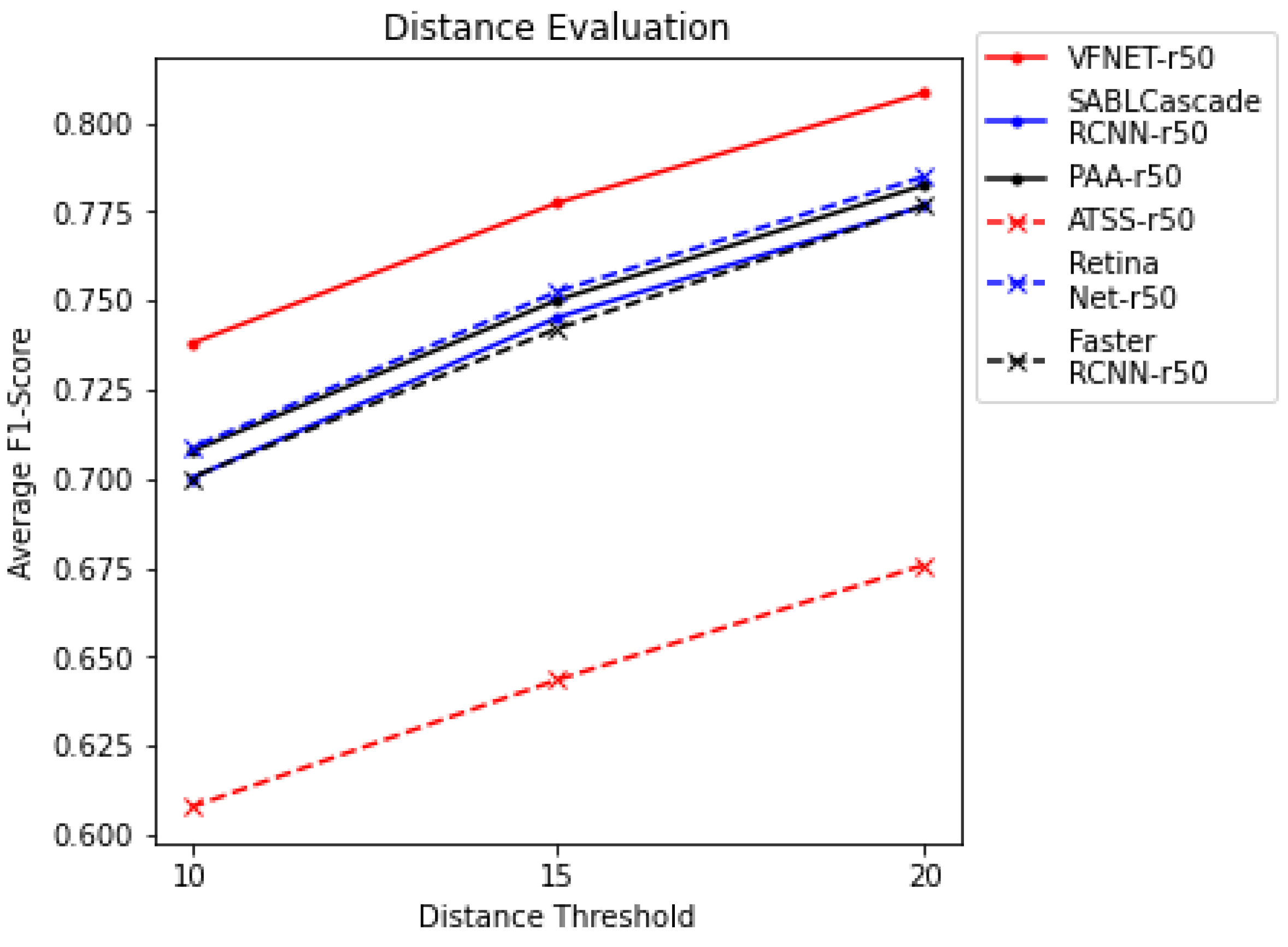
Figure 6 presents the F1-Score (average) considering all folds (F1-F5) and bounding boxes sizes (10 × 10 to 50 × 50 pixels) for three distance threshold values of 10 (550 m), 15 (825 m), and 20 pixels (1100 m). As expected, the F1 decreased considering 10 and 15 pixels compared to 20 pixels. In practical terms, this distance is acceptable because it is possible to easily see the location of the fire in Pantanal due to its flat terrain that can make it easier for firefighters to see the focus. Hence, the 20 pixels threshold was adopted for analyses. VFNET presents the highest average F1-Score based on this global result, achieving 0.81 when considering the threshold distance equal to 20 pixels (1100 m). The ATSS has the lowest F1-Score values due to the lowest recall values (few TP bounding boxes and many FN bounding boxes), while the remaining algorithms provided competitive results. According to these results, the increase of the distance threshold allows accepting more distant predictions from ground-truth, which increases the number of true positives. However, the average distance between the predicted and ground-truth bounding boxes also increases. In this sense, Table 3 shows the distance of the predictions (those whose score values are above 0.5) to the closest ground-truth bounding boxes (considering the TP and FP predictions). This average result shows that the highest average distance, around 14.5 pixels (797.5 m), achieved by the PAA method is inside the maximum allowed distance (threshold equal to 20 pixels). The ATSS achieves the lowest distances (4.4 pixels). The remaining methods show competitive results with distance values around 7.4 and 9.8 pixels. In summary, the VFNET achieves a good balance between precision and recall and the closest distances near the mean distance values (8.87 pixels) among the methods.
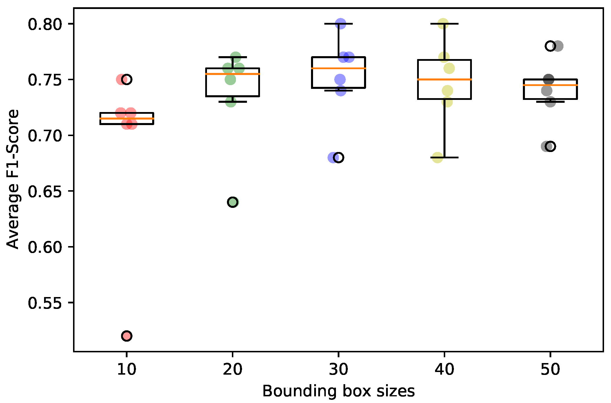
Figure 7 shows the average F1-Score variation over each bounding box size evaluated, and the colored circles represent a calculated value to each method to build the box plot. It is possible to notice that the objects with squared bounding boxes with 10 × 10 pixels produce the worst F1 values, which occurs due to the insufficient information about the smoke plume inside these tiny squared bounding boxes to train the detection methods. The best results are achieved with squared boxes of sizes 30 and 40 pixels with an average F1-Score value around 0.80. The colored dots in each box plot represent the F1-Score values of each algorithm. In this sense, the dots near the minimum value of each box represent the ATSS, which achieve the lowest F1-Score values in all bounding boxes sizes. However, even considering the results for the ATSS algorithm, it is possible to observe the increase of the F1-Score from 10 to 30 pixels and that these values stabilize between 30 and 50 pixels. According to these results, the best sizes of the squared bounding box are 30 and 40, which achieved an F1-Score equal to 0.83 with the VFNET algorithm, considering the threshold distance equal to 20 pixels (Figure 8). When squared boxes are increased beyond 50 pixels, the overlap between bounding boxes increases, and more irrelevant information around the smoke plumes are considered in the training process, which may confuse the algorithms to learn the objects of interest.

3.2. Qualitative Analysis and Discussion

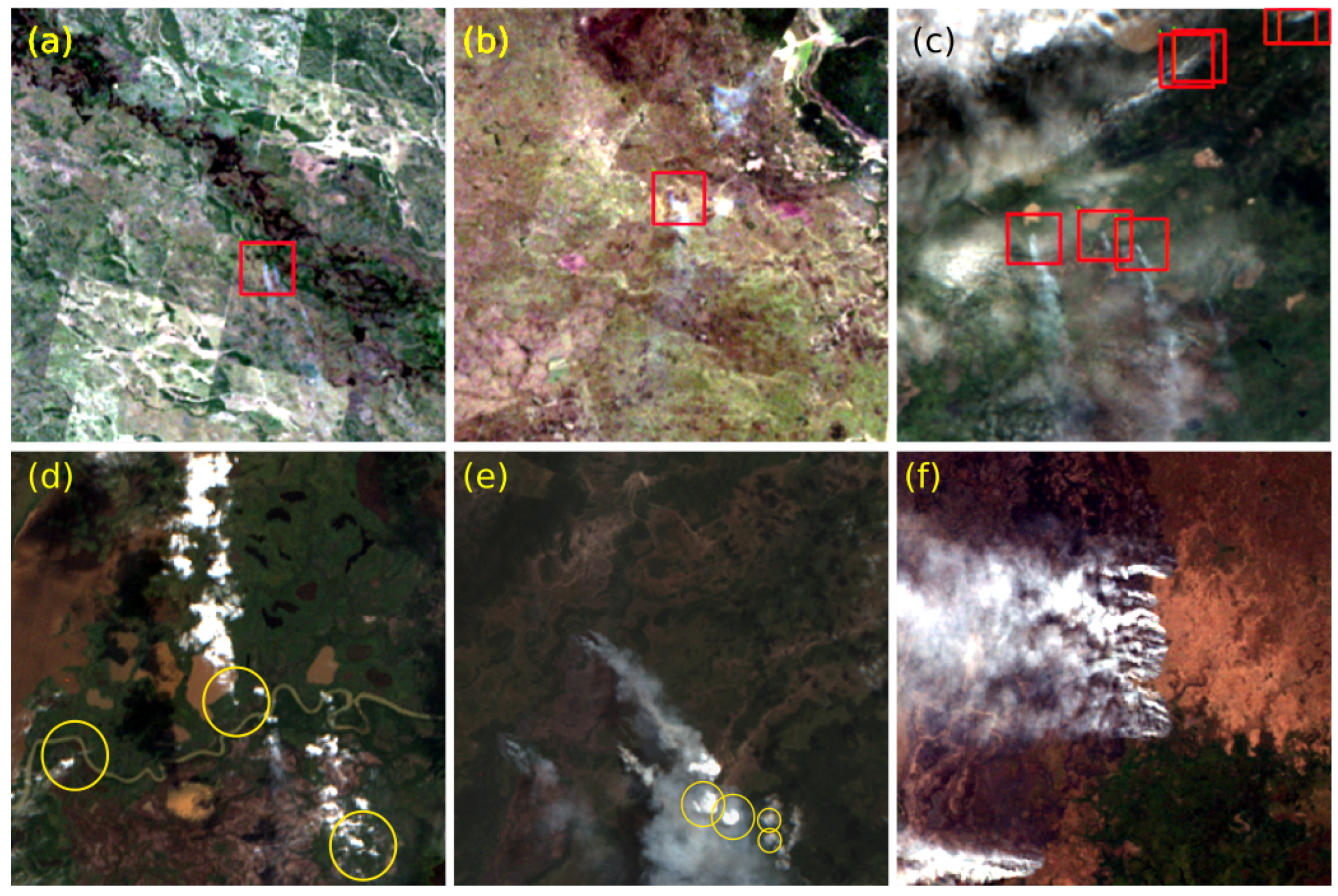
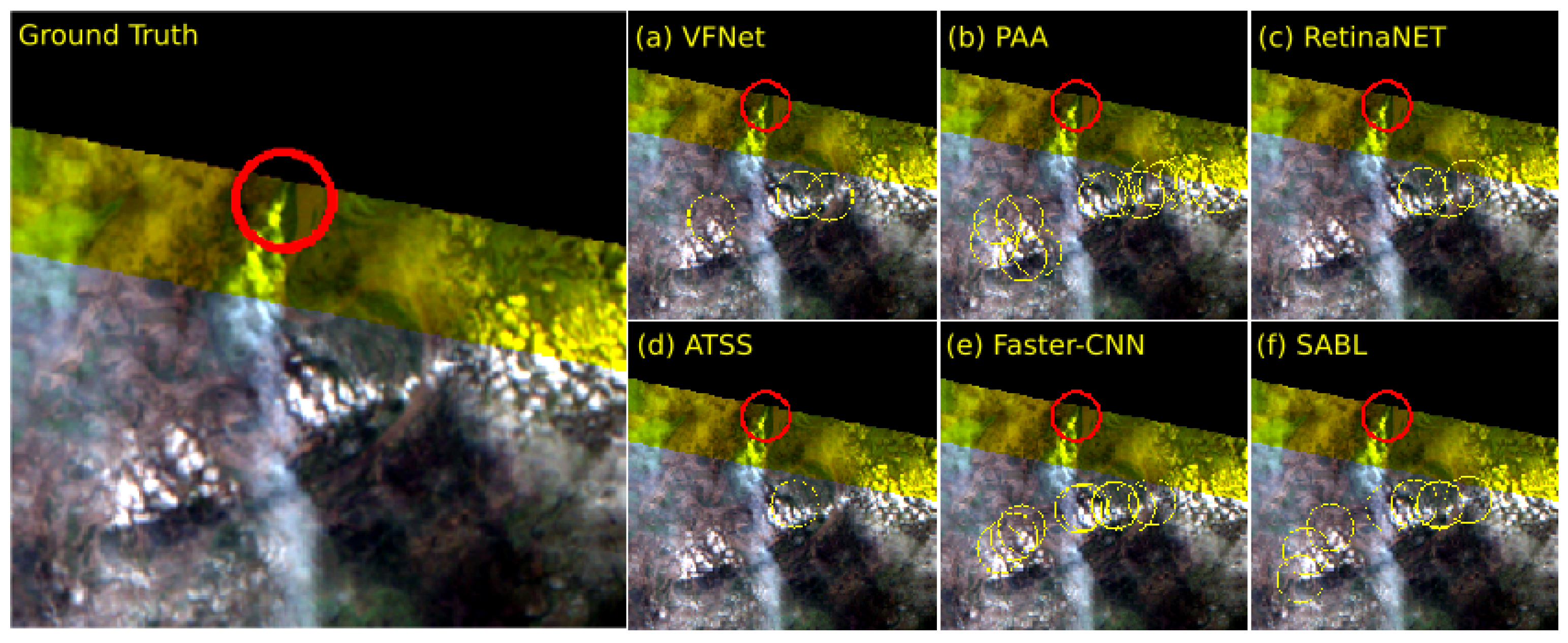
Another perspective is to evaluate results qualitatively. Therefore, we visually analyzed the methods assertiveness for smoke plumes detection over different conditions, as shown in Figure 9, such as small smoke plumes (small areas), round plumes not affected by wind spreads (almost orthogonal dispersion), smoke plumes above thin clouds coverage (may cause pixel response confusion), clouds with plume format, fine smoke plumes, small dense clouds, and overlapped or mixed plumes from another smoke plume. The visual perception among positive, false-positive, and non-identification results are shown in this section and refers to 40 squared bounding boxes in fold 1, as provided the most accurate result.
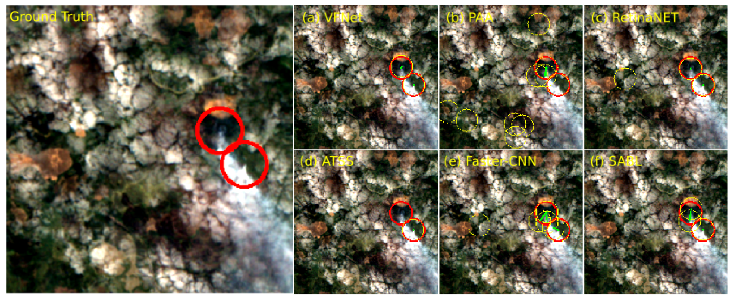
The positive results of all methods vary from easy detections, with clear smoke boundaries and good background contrast (Figure 10), to difficult identifications with mixed smoke and cloud coverage (Figure 11). Moreover, some methods performed very complex detections as moderate cloud coverage, multiple plumes, or even some that may cause doubt for human operators.
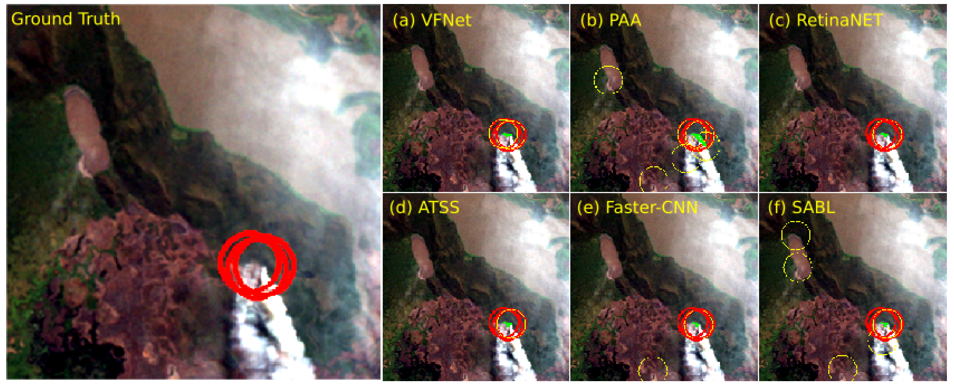
In general, we observed that a FP higher frequency occurs from image cloud coverage caused by format and density that may confuse the detection. It is possible to observe (Figure 11) the predicted bounding circles (in red) and the annotated bounding circles (in green) for each evaluated algorithm on fold 1. In this scenario, the presence of clouds, which are visually similar to the smoke plume, confuses the algorithms SABL, Faster RCNN, and PAA. The Retinanet, ATSS, and VFNET algorithms accurately detect the smoke plumes. In the same way, cone-shaped or concentrated rounds clouds lead to object identification errors. The lower false positive frequency was related to tiled clouds from patches and terrestrial features with high albedo. The image tiles may cause cloud cut, creating cone-shaped clouds, since one side of the cloud appears linear in the patch. The terrestrial features had combined thin linear or smoke-shaped and high albedo, the similar spectral response and shape of some smoke plumes (Figure 10b,f).
The higher number of non-identified smoke plumes were multiple small plumes (Figure 12), being some of them cloud covered. In addition, a few non-identified smoke plumes are related to bands misalignment, which leads to non-identification since the image is not RBG entirely composed (Figure 13).
Visually, among the methods, VFNET presented fewer FP (Figure 14) that justify its best quantitative results obtained. The PAA showed a high sensitive detection (Figure 14) since the boxes selection was probabilistic based, which may raise the FP identification, despite its good performance.
To interpret what the algorithms are learning, we apply the gradient-weighted class activation mapping plus plus (Grad-CAM++) [48] to visualize important regions in the last layer of the Resnet-50 of each algorithm. In Figure 15, the original image and the class activation map (heatmap) for the SABL, Faster-RCNN, and PAA, respectively, are presented. It is possible to note that the smoke plume has a high confidence score to be an object of interest, highlighted in red. However, some clouds also have a significant confidence score to be an object of interest. Considering the ATSS algorithm, the smoke plumes also have a high confidence score compared with the remaining areas where the clouds exist, but less intense than other algorithms (not so red). The RetinaNet and VFNET reduce the importance of regions with clouds and highlight the smoke plumes with the highest confidence score.
Despite those FP detections, it is relevant to emphasize that even human operators can be confused in these identification samples. We noticed that the CNNs evaluated identified some smoke plumes not annotated or not assuredly identified and not annotated.
The FP or non-identified smoke plumes probably are mainly caused by atmospheric and weather effects since the imagery dataset has a wide range of cloud cover rates. It is also important to mention that although such cloud covered optical images are usually not of sufficient quality for traditional land use and land cover mapping initiatives, such images are still important for early warning systems of fire events, such as presented herein.
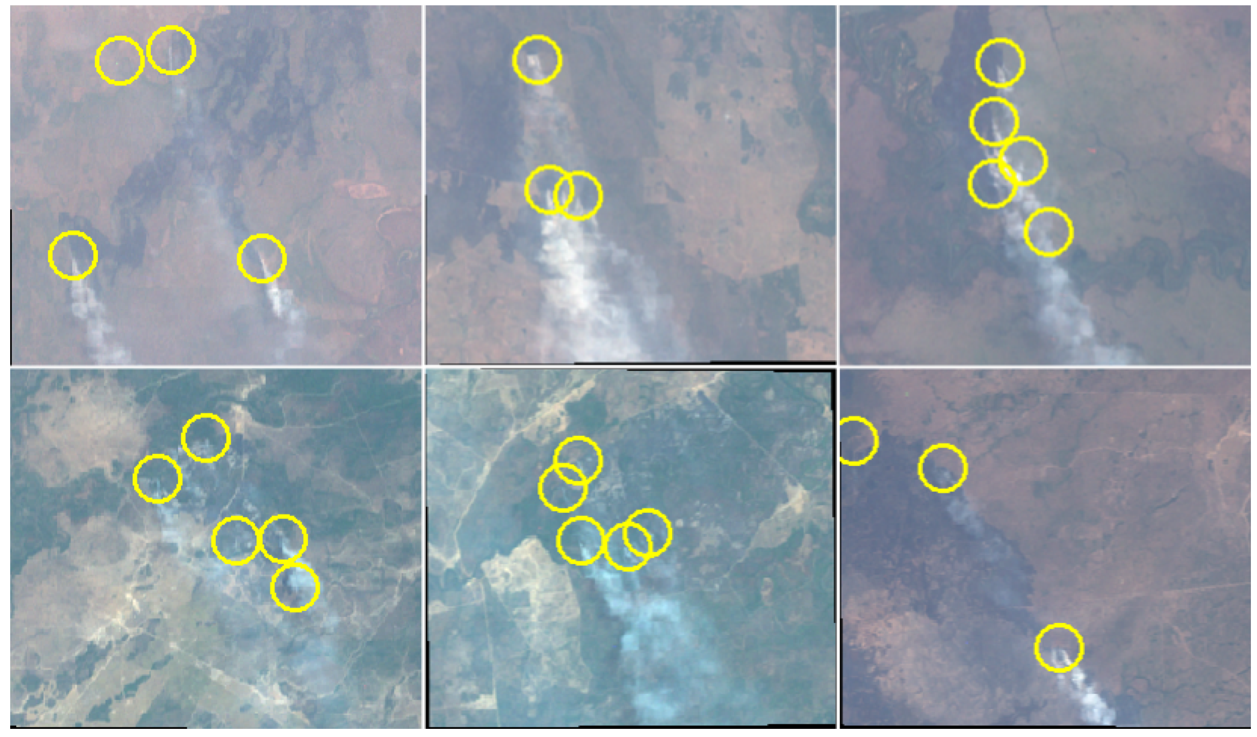
In order to verify the generalization capability of the model, trained on images from 2020, we applied inference on images from 2021. Figure 16 shows the prediction results from the best model configuration discussed in previous sections. We verified that the model provided the detection of most active fires, showing good performance even with images acquired in different years. It is important to highlight also the variability of the proposed dataset that significantly contributed to this achievement.
To summarize, our results indicate that VFNET provided the highest F1-Score, followed by RetinaNet, SABL, Faster R-CNN, and ATSS. Previous studies in remote sensing [49,50] showed that ATSS provided more accurate results for pole and apple detection; however, for active fire detection, ATSS provided less accurate results due to a small rate of True Positives, indicating the inability of the trained model (considering the same number of training epochs of the remaining algorithms) to identify active fire regions.

3.3. Comparison with BD Queimadas Database

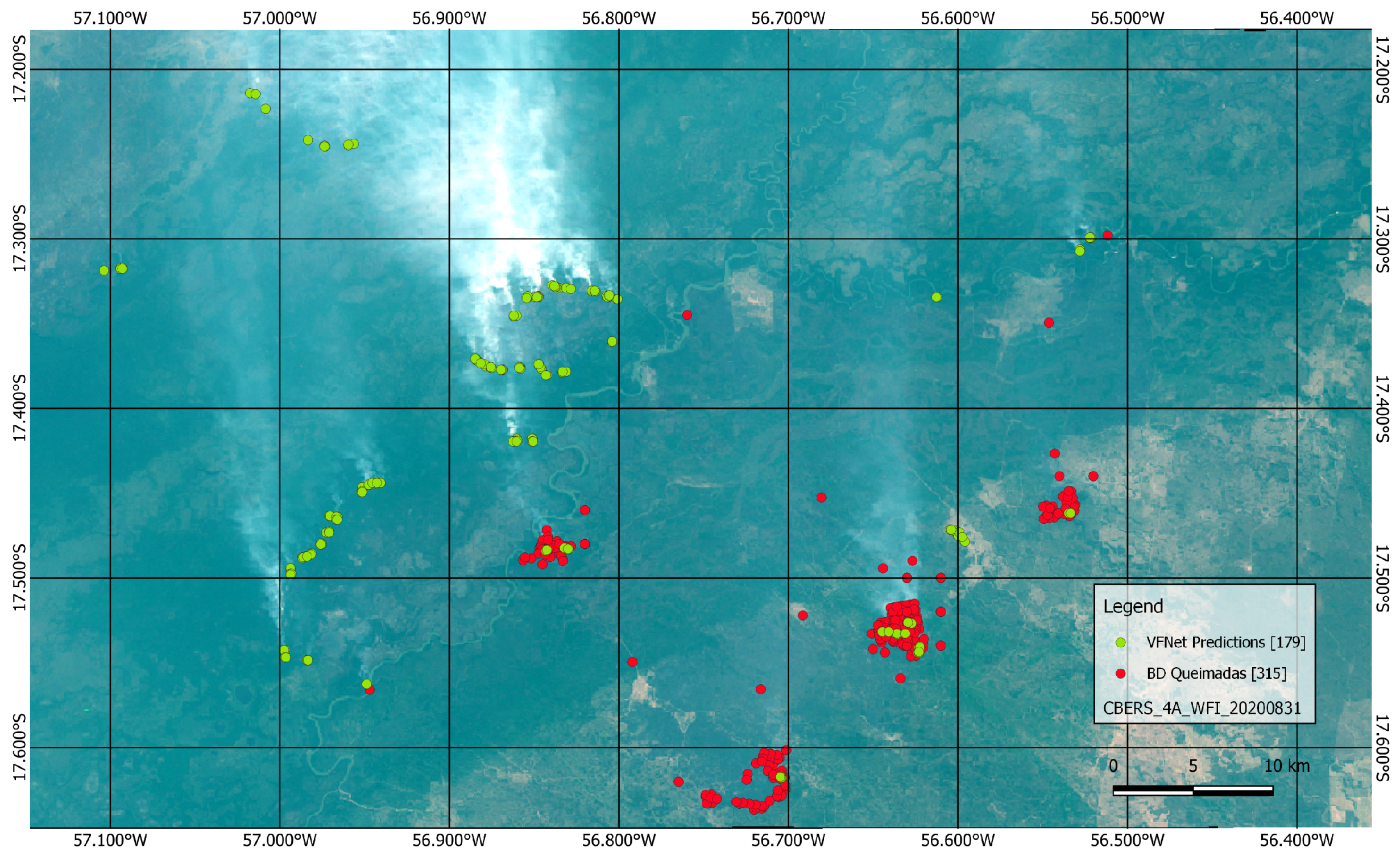
In this section, we evaluate the effectiveness of the VFNET model (trained with images from fold 1 with bounding box of size 40) on CBERS 4A WFI (31 August 2020) and compare with BD Queimadas data (heat points from 31 August 2020). Figure 17 depicts CBERS 4A, the predicted VFNet fire (yellow), and the BD Queimadas data (red).
Table 4 presents the results in terms of Precision, Recall, F1-Score, and average distances between the center of predicted bounding boxes and its closest ground-truth bounding box center. We can observe that the VFNET obtains a F1-Score value of 0.84, showing a good trade-off between Precision and Recall. In addition, the centers of predicted bounding boxes are very close to the ground truths, highlighting the potential of the VFNET method to identify smoke plume fire activities.
Qualitatively, it is possible to notice that BD Queimadas data (Figure 17) detected a higher number of smoke plumes than VFNet. However, the detection shows clustered points and misses some fire detections. VFNet data predicted a minor number of plumes but with a higher number of active fire assertiveness. So these results show that the proposed approach can be useful as a complementary method to the thermal-based active fire detection methods.

4. Conclusions

We proposed a deep learning-based approach based on points to detect active fires on satellite images for the Brazilian Pantanal. Six methods were evaluated, including the commonly used Faster R-CNN and RetinaNet, on the CBERS 4A WFI imagery. Since the smoke plumes were hand-annotated with points, we evaluated the impact of the bounding box size on the detection. Extensive experiments were conducted, generating a total of 150 models. We provided quantitative analysis and qualitative analysis for these models.
Our results indicate that the bounding box sizes of 30 or 40 pixels presented the best performance. Finally, our findings show that VFNET provided the highest F1-Score, followed by RetinaNet, SABL, and Faster R-CNN. The ATSS showed the worst average performance.
The proposed deep learning-based method to detect smoke plumes (active fire) in remote sense data presents promising results and could be a useful complementary approach to identifying smoke plumes to other research and wildfire databases such as BD Queimadas (INPE) with higher spatial resolution, despite the five-day scan time-lapse. Furthermore, developing new techniques and solutions, aggregated with the well-established references, as BD Queimadas, can be important to improve the response in wildfire firefighting, environmental protection, and forensics investigation. Further studies are expected to employ this proposed method in other challenging ecosystems where the detection of smoke plumes is still a required information in fire fighting and rescue initiatives.

Author Contributions

Conceptualization, L.H., J.M.J., V.L., W.N.G. and J.S.; Data curation, L.H., R.S. and R.L.; Formal analysis, V.L.; Funding acquisition, J.M.J., V.L., F.R. and R.L.; Investigation, L.H. and T.R.; Methodology, L.H., J.M.J., P.Z., L.A., V.L., R.L., W.N.G. and J.S.; Project administration, F.R. and R.L.; Software, P.Z., R.S., L.A., W.N.G. and J.S.; Supervision, J.M.J. and T.R.; Validation, L.H. and W.N.G.; Writing—original draft, L.H., J.M.J., W.N.G. and J.S.; Writing—review & editing, T.R., P.Z., R.S., L.A., V.L., F.R. and R.L. All authors have read and agreed to the published version of the manuscript.

Funding

This research was funded by CNPq (p: 313887/2018-7, 433783/2018-4, 304052/2019-1, and 303559/2019-5), FUNDECT (p: 59/300.066/2015), CAPES PrInt (p: 88881.311850/2018-01) and Project Rede Pantanal from the Ministry of Science, Technology, and Innovations of Brazil (FINEP Grant No. 01.20.0201.00). The authors acknowledge the support of the UFMS (Federal University of Mato Grosso do Sul) and CAPES (Finance Code 001). V. Liesenberg is supported by FAPESC (2017TR1762).

Data Availability Statement

The dataset is available at https://sites.google.com/view/geomatics-and-computer-vision/home/datasets, accessed on 10 December 2021.

Acknowledgments

The authors would like to acknowledge NVidia for their donation of the Titan X graphics card used in the experiments.

Conflicts of Interest

The authors declare no conflict of interest.

References

  1. Calheiros, D.F.; Oliveira, M.; Padovani, C.R. Hydro-ecological processes and anthropogenic impacts on the ecosystem services of the Pantanal wetland. In Tropical Wetland Management: The South-American Pantanal and the International Experience; Routledge: London, UK, 2012; pp. 29–57. [Google Scholar]
  2. da Silva, J.B.; Junior, L.C.G.V.; Faria, T.O.; Marques, J.B.; Dalmagro, H.J.; Nogueira, J.S.; Vourlitis, G.L.; Rodrigues, T.R. Temporal variability in evapotranspiration and energy partitioning over a seasonally flooded scrub forest of the Brazilian Pantanal. Agric. For. Meteorol. 2021, 308, 108559. [Google Scholar] [CrossRef]
  3. do Brasil, S.F. Constituição da República Federativa do Brasil; Senado Federal, Centro Gráfico: Brasília, Brazil, 1988. [Google Scholar]
  4. Alho, C.J.; Sabino, J. Seasonal Pantanal flood pulse: Implications for biodiversity. Oecologia Aust. 2012, 16, 958–978. [Google Scholar] [CrossRef] [Green Version]
  5. Junk, W.J.; Da Cunha, C.N.; Wantzen, K.M.; Petermann, P.; Strüssmann, C.; Marques, M.I.; Adis, J. Biodiversity and its conservation in the Pantanal of Mato Grosso, Brazil. Aquat. Sci. 2006, 68, 278–309. [Google Scholar] [CrossRef]
  6. Braz, A.M.; Melo, D.S.; Boni, P.V.; Decco, H.F. A estrutura fundiária do pantanal brasileiro. Finisterra 2020, 55, 157–174. [Google Scholar]
  7. INPE. Portal do Monitoramento de Queimadas e Incêndios Florestais. 2020. Available online: http://www.inpe.br/queimadas (accessed on 1 September 2019).
  8. Xu, W.; Liu, Y.; Veraverbeke, S.; Wu, W.; Dong, Y.; Lu, W. Active Fire Dynamics in the Amazon: New Perspectives From High-Resolution Satellite Observations. Geophys. Res. Lett. 2021, 48, e2021GL093789. [Google Scholar] [CrossRef]
  9. Deng, J.; Dong, W.; Socher, R.; Li, L.J.; Li, K.; Fei-Fei, L. Imagenet: A large-scale hierarchical image database. In Proceedings of the 2009 IEEE Conference on Computer Vision and Pattern Recognition, Miami, FL, USA, 20–25 June 2009; IEEE: Piscataway, NJ, USA, 2009; pp. 248–255. [Google Scholar]
  10. Everingham, M.; Van Gool, L.; Williams, C.K.; Winn, J.; Zisserman, A. The pascal visual object classes (voc) challenge. Int. J. Comput. Vis. 2010, 88, 303–338. [Google Scholar] [CrossRef] [Green Version]
  11. Lin, T.Y.; Maire, M.; Belongie, S.; Hays, J.; Perona, P.; Ramanan, D.; Dollár, P.; Zitnick, C.L. Microsoft coco: Common objects in context. In Proceedings of the European Conference on Computer Vision, Zurich, Switzerland, 6–12 September 2014; Springer: Berlin/Heidelberg, Germany, 2014; pp. 740–755. [Google Scholar]
  12. Zhou, W.; Newsam, S.; Li, C.; Shao, Z. PatternNet: A benchmark dataset for performance evaluation of remote sensing image retrieval. ISPRS J. Photogramm. Remote Sens. 2018, 145, 197–209. [Google Scholar] [CrossRef] [Green Version]
  13. Li, K.; Wan, G.; Cheng, G.; Meng, L.; Han, J. Object detection in optical remote sensing images: A survey and a new benchmark. ISPRS J. Photogramm. Remote Sens. 2020, 159, 296–307. [Google Scholar] [CrossRef]
  14. Jain, P.; Coogan, S.C.; Subramanian, S.G.; Crowley, M.; Taylor, S.; Flannigan, M.D. A review of machine learning applications in wildfire science and management. Environ. Rev. 2020, 28, 478–505. [Google Scholar] [CrossRef]
  15. Barmpoutis, P.; Papaioannou, P.; Dimitropoulos, K.; Grammalidis, N. A review on early forest fire detection systems using optical remote sensing. Sensors 2020, 20, 6442. [Google Scholar] [CrossRef]
  16. Zhang, Q.; Xu, J.; Xu, L.; Guo, H. Deep convolutional neural networks for forest fire detection. In Proceedings of the 2016 International Forum on Management, Education and Information Technology Application, Guangzhou, China, 30–31 January 2016; Atlantis Press: Dordrecht, The Netherlands, 2016. [Google Scholar]
  17. Wahyuni, E.S.; Hendri, M. Smoke and Fire Detection Base on Convolutional Neural Network. ELKOMIKA J. Tek. Energi Elektr. Tek. Telekomun. Tek. Elektron. 2019, 7, 455. [Google Scholar] [CrossRef]
  18. Wang, Y.; Dang, L.; Ren, J. Forest fire image recognition based on convolutional neural network. J. Algorithms Comput. Technol. 2019, 13, 1748302619887689. [Google Scholar] [CrossRef] [Green Version]
  19. Pan, H.; Badawi, D.; Zhang, X.; Cetin, A.E. Additive neural network for forest fire detection. Signal Image Video Process. 2019, 14, 675–682. [Google Scholar] [CrossRef]
  20. Chen, Y.; Zhang, Y.; Xin, J.; Yi, Y.; Liu, D.; Liu, H. A UAV-based forest fire detection algorithm using convolutional neural network. In Proceedings of the 2018 37th Chinese Control Conference (CCC), Wuhan, China, 25–27 July 2018; IEEE: Piscataway, NJ, USA, 2018; pp. 10305–10310. [Google Scholar]
  21. Jiao, Z.; Zhang, Y.; Xin, J.; Mu, L.; Yi, Y.; Liu, H.; Liu, D. A deep learning based forest fire detection approach using UAV and YOLOv3. In Proceedings of the 2019 1st International Conference on Industrial Artificial Intelligence (IAI), Shenyang, China, 22–26 July 2019; IEEE: Piscataway, NJ, USA, 2019; pp. 1–5. [Google Scholar]
  22. Lee, W.; Kim, S.; Lee, Y.T.; Lee, H.W.; Choi, M. Deep neural networks for wild fire detection with unmanned aerial vehicle. In Proceedings of the 2017 IEEE international conference on consumer electronics (ICCE), Taipei, Taiwan, 12–14 June 2017; IEEE: Piscataway, NJ, USA, 2017; pp. 252–253. [Google Scholar]
  23. Govil, K.; Welch, M.L.; Ball, J.T.; Pennypacker, C.R. Preliminary results from a wildfire detection system using deep learning on remote camera images. Remote Sens. 2020, 12, 166. [Google Scholar] [CrossRef] [Green Version]
  24. Vani, K. Deep learning based forest fire classification and detection in satellite images. In Proceedings of the 2019 11th International Conference on Advanced Computing (ICoAC), Chennai, India, 8–20 December 2019; IEEE: Piscataway, NJ, USA, 2019; pp. 61–65. [Google Scholar]
  25. Ba, R.; Chen, C.; Yuan, J.; Song, W.; Lo, S. Smokenet: Satellite smoke scene detection using convolutional neural network with spatial and channel-wise attention. Remote Sens. 2019, 11, 1702. [Google Scholar] [CrossRef] [Green Version]
  26. Pinto, M.M.; Libonati, R.; Trigo, R.M.; Trigo, I.F.; DaCamara, C.C. A deep learning approach for mapping and dating burned areas using temporal sequences of satellite images. ISPRS J. Photogramm. Remote Sens. 2020, 160, 260–274. [Google Scholar] [CrossRef]
  27. Wang, J.; Zhang, W.; Cao, Y.; Chen, K.; Pang, J.; Gong, T.; Shi, J.; Loy, C.C.; Lin, D. Side-aware boundary localization for more precise object detection. In Proceedings of the European Conference on Computer Vision, Glasgow, UK, 23–28 August 2020; Springer: Berlin/Heidelberg, Germany, 2020; pp. 403–419. [Google Scholar]
  28. Zhang, S.; Chi, C.; Yao, Y.; Lei, Z.; Li, S.Z. Bridging the gap between anchor-based and anchor-free detection via adaptive training sample selection. In Proceedings of the IEEE/CVF Conference on Computer Vision and Pattern Recognition, Seattle, WA, USA, 14–19 June 2020; pp. 9759–9768. [Google Scholar]
  29. Zhang, H.; Wang, Y.; Dayoub, F.; Sunderhauf, N. Varifocalnet: An iou-aware dense object detector. In Proceedings of the IEEE/CVF Conference on Computer Vision and Pattern Recognition, New Orleans, LA, USA, 19–24 June 2021; pp. 8514–8523. [Google Scholar]
  30. Kim, K.; Lee, H.S. Probabilistic anchor assignment with iou prediction for object detection. In Proceedings of the Computer Vision–ECCV 2020: 16th European Conference, Glasgow, UK, 23–28 August 2020; Proceedings, Part XXV 16. Springer: Berlin/Heidelberg, Germany, 2020; pp. 355–371. [Google Scholar]
  31. Gef (Global Environment Facility) Pantanal/Upper Paraguay Project. Implementation of Integrated River Basin Management Practices in the Pantanal and Upper Paraguay River Basin. Strategic Action Program for the Integrated Management of the Pantanal and Upper Paraguay River Basin. ANA/GEF/UNEP/OAS; TDA Desenho & Arte Ltda: Brasilia, Brazil, 2004; 63p. [Google Scholar]
  32. Alvares, C.A.; Stape, J.L.; Sentelhas, P.C.; Gonçalves, J.d.M.; Sparovek, G. Köppen’s climate classification map for Brazil. Meteorol. Z. 2013, 22, 711–728. [Google Scholar] [CrossRef]
  33. IBGE. Biomas. 2020. Available online: https://www.ibge.gov.br/geociencias/informacoes-ambientais/vegetacao/15842-biomas.html?=&t=downloads (accessed on 1 September 2019).
  34. INPE. CBERS 4A. 2020. Available online: http://www.cbers.inpe.br/sobre/cbers04a.php (accessed on 1 September 2019).
  35. Abuelgasim, A.; Fraser, R. Day and night-time active fire detection over North America using NOAA-16 AVHRR data. In Proceedings of the IEEE International Geoscience and Remote Sensing Symposium, Honolulu, HI, USA, 25–30 July 2010; IEEE: Piscataway, NJ, USA, 2002; Volume 3, pp. 1489–1491. [Google Scholar]
  36. Christopher, S.A.; Wang, M.; Barbieri, K.; Welch, R.M.; Yang, S.K. Satellite remote sensing of fires, smoke and regional radiative energy budgets. In Proceedings of the 1997 IEEE International Geoscience and Remote Sensing Symposium Proceedings, IGARSS’97, Remote Sensing—A Scientific Vision for Sustainable Development, Singapore, 3–8 August 1997; Volume 4, pp. 1923–1925. [Google Scholar]
  37. Giglio, L.; Descloitres, J.; Justice, C.O.; Kaufman, Y.J. An enhanced contextual fire detection algorithm for MODIS. Remote Sens. Environ. 2003, 87, 273–282. [Google Scholar] [CrossRef]
  38. Ren, S.; He, K.; Girshick, R.; Sun, J. Faster r-cnn: Towards real-time object detection with region proposal networks. Adv. Neural Inf. Process. Syst. 2015, 28, 91–99. [Google Scholar] [CrossRef] [Green Version]
  39. Lin, T.Y.; Goyal, P.; Girshick, R.; He, K.; Dollár, P. Focal loss for dense object detection. In Proceedings of the IEEE International Conference on Computer Vision, Venice, Italy, 22–29 October 2017; pp. 2980–2988. [Google Scholar]
  40. Lin, T.Y.; Dollár, P.; Girshick, R.; He, K.; Hariharan, B.; Belongie, S. Feature pyramid networks for object detection. In Proceedings of the IEEE Conference on Computer Vision and Pattern Recognition, Honolulu, HI, USA, 21–26 July 2017; pp. 2117–2125. [Google Scholar]
  41. Tian, Z.; Shen, C.; Chen, H.; He, T. Fcos: Fully convolutional one-stage object detection. In Proceedings of the IEEE/CVF International Conference on Computer Vision, Seoul, Korea, 27–28 October 2019; pp. 9627–9636. [Google Scholar]
  42. Dai, J.; Qi, H.; Xiong, Y.; Li, Y.; Zhang, G.; Hu, H.; Wei, Y. Deformable convolutional networks. In Proceedings of the IEEE International Conference on Computer Vision, Venice, Italy, 22–29 October 2017; pp. 764–773. [Google Scholar]
  43. Zhang, X.; Wan, F.; Liu, C.; Ji, R.; Ye, Q. Freeanchor: Learning to match anchors for visual object detection. arXiv 2019, arXiv:1909.02466. [Google Scholar]
  44. Ke, W.; Zhang, T.; Huang, Z.; Ye, Q.; Liu, J.; Huang, D. Multiple anchor learning for visual object detection. In Proceedings of the IEEE/CVF Conference on Computer Vision and Pattern Recognition, Seattle, WA, USA, 14–19 June 2020; pp. 10206–10215. [Google Scholar]
  45. Li, H.; Wu, Z.; Zhu, C.; Xiong, C.; Socher, R.; Davis, L.S. Learning from noisy anchors for one-stage object detection. In Proceedings of the IEEE/CVF Conference on Computer Vision and Pattern Recognition, Seattle, WA, USA, 14–19 June 2020; pp. 10588–10597. [Google Scholar]
  46. Chen, K.; Wang, J.; Pang, J.; Cao, Y.; Xiong, Y.; Li, X.; Sun, S.; Feng, W.; Liu, Z.; Xu, J.; et al. MMDetection: Open MMLab Detection Toolbox and Benchmark. arXiv 2019, arXiv:1906.07155. [Google Scholar]
  47. Kuhn, H.W. The Hungarian Method for the Assignment Problem. Nav. Res. Logist. Q. 1955, 2, 83–97. [Google Scholar] [CrossRef] [Green Version]
  48. Chattopadhay, A.; Sarkar, A.; Howlader, P.; Balasubramanian, V.N. Grad-cam++: Generalized gradient-based visual explanations for deep convolutional networks. In Proceedings of the 2018 IEEE Winter Conference on Applications of Computer Vision (WACV), Lake Tahoe, NV, USA, 12–15 March 2018; IEEE: Piscataway, NJ, USA, 2018; pp. 839–847. [Google Scholar]
  49. Gomes, M.; Silva, J.; Gonçalves, D.; Zamboni, P.; Perez, J.; Batista, E.; Ramos, A.; Osco, L.; Matsubara, E.; Li, J.; et al. Mapping Utility Poles in Aerial Orthoimages Using ATSS Deep Learning Method. Sensors 2020, 20, 6070. [Google Scholar] [CrossRef]
  50. Biffi, L.J.; Mitishita, E.; Liesenberg, V.; Santos, A.A.d.; Gonçalves, D.N.; Estrabis, N.V.; Silva, J.d.A.; Osco, L.P.; Ramos, A.P.M.; Centeno, J.A.S.; et al. ATSS Deep Learning-Based Approach to Detect Apple Fruits. Remote Sens. 2021, 13, 54. [Google Scholar] [CrossRef]
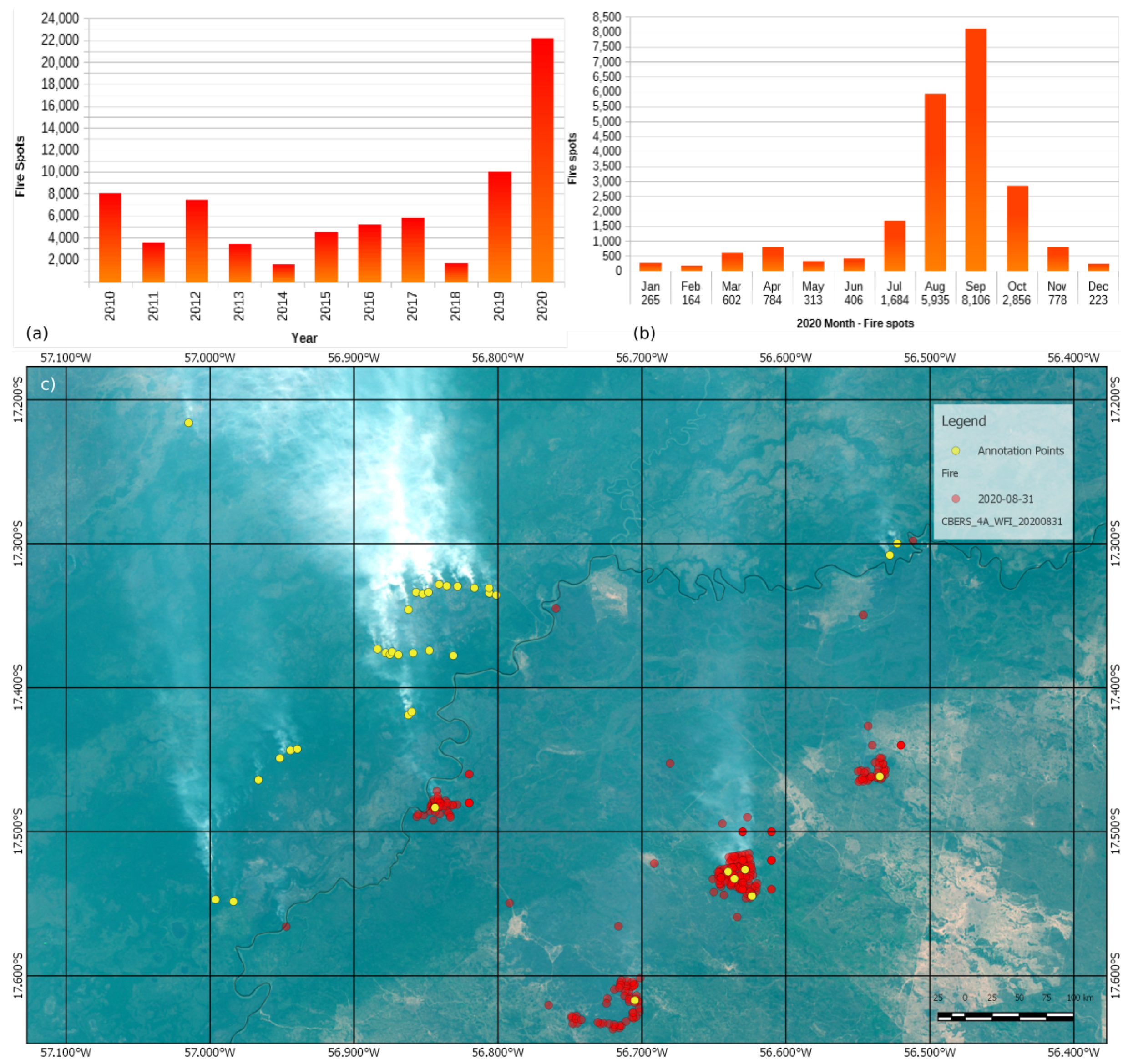
Figure 1. (a) BD Queimadas data of active fire in Pantanal in the last decade and (b) the Queimadas database active fire from January to December 2020, and (c) CBERS 04A, Queimadas active fire (red dots), and manual annotation (yellow dots).
Remotesensing 14 00688 g001
Figure 2. Study area location: (left) South America and Brazil; (right upper) Brazil; and (right lower) study area (Brazilian Pantanal).
Remotesensing 14 00688 g002
Figure 3. (a) Points and boxes; (b) points; and (c) boxes legend.
Remotesensing 14 00688 g003
Figure 4. Workflow of the proposed method.
Remotesensing 14 00688 g004
Figure 5. Example of Precision and Recall estimation to a distance threshold equal to 20. There are four predicted fire regions (represented as yellow circles) and four annotated fire regions (represented as red circles).
Remotesensing 14 00688 g005
Figure 6. The average F1-Score values for all algorithms for each distance threshold.
Remotesensing 14 00688 g006
Figure 7. Average F1-Score considering all distance thresholds (10, 15, and 20 pixels).
Remotesensing 14 00688 g007
Figure 8. Average F1-Score considering the distance threshold equal to 20 pixels.
Remotesensing 14 00688 g008
Figure 9. Ground-truth examples of (a) small smoke plumes, (b) smoke almost perpendicular dispersion, (c) smoke plumes above thin clouds, (d) cloud plume format (yellow rounds), (e) small dense clouds (yellow rounds), and (f) overlapped or mixed plumes.
Remotesensing 14 00688 g009
Figure 10. Easy detection with good background contrast and smoke boundaries (Ground-truth—red rounds and prediction—green rounds).
Remotesensing 14 00688 g010
Figure 11. Difficult detection with clouds coverage mixed with smoke (ground truth—red rounds and prediction—green rounds).
Remotesensing 14 00688 g011
Figure 12. Ground-truth (red rounds) and prediction (green rounds) of terrestrial features with high albedo detected by PAA and SABL. Multiple plumes are also presented.
Remotesensing 14 00688 g012
Figure 13. Band stripping misalignment. Ground truth (red rounds) and prediction (green rounds) of false positive detection due to cloud format and density.
Remotesensing 14 00688 g013
Figure 14. Ground-truth (red rounds) and prediction (green rounds). Few false-positive detection of VFNET and highly sensitive for PAA.
Remotesensing 14 00688 g014
Figure 15. Original image and the Grad-CAM++ activation map (heatmap) for each method.
Remotesensing 14 00688 g015
Figure 16. Predicted regions with active fire on six patches from images acquired in 2021.
Remotesensing 14 00688 g016
Figure 17. CBERS 4A image subset (31 August 2020), the predicted VFNet fire, and the BD Queimadas data.
Remotesensing 14 00688 g017
Table 1. CBERS 4A Imagery date, path, row, and correction level.
DatePathRowLevelDatePathRowLevel
4 May 2020214140L421 July 2020217132L4
5 May 2020220132L221 July 2020217140L4
5 May 2020220140L222 July 2020223132L4
10 May 2020219140L426 July 2020216132L4
15 May 2020218140L426 July 2020216140L4
20 May 2020217132L427 July 2020222132L4
20 May 2020217140L427 July 2020222140L4
31 May 2020221140L431 July 2020215132L4
10 June 2020219132L41 August 2020221132L4
10 June 2020219140L41 August 2020221140L4
15 June 2020218132L45 August 2020214140L4
15 June 2020218140L46 August 2020220132L4
20 June 2020217132L46 August 2020220140L4
20 June 2020217140L410 August 2020213132L4
25 June 2020216132L410 August 2020213140L4
30 June 2020215132L411 August 2020219132L4
30 June 2020215140L411 August 2020219140L2
1 July 2020221132L415 August 2020212132L4
1 July 2020221140L416 August 2020218132L4
5 July 2020214140L426 August 2020216132L4
6 July 2020220132L426 August 2020216140L4
11 July 2020219132L427 August 2020222132L4
15 July 2020212140L431 August 2020215132L4
16 July 2020218132L431 August 2020215140L4
16 July 2020218140L4
Table 2. Description of the training, validation, and test sets of the active fire dataset.
FoldTestTrainValidation
PatchesImagesPatchesImagesPatchesImages
F179 (10%)10497 (64%)28199 (26%)10
F282 (11%)10493 (64%)28200 (26%)10
F3187 (24%)10437 (56%)28151 (19%)10
F4182 (23%)9360 (46%)29233 (30%)10
F5245 (32%)9371 (48%)29159 (21%)10
Table 3. Average distances (and its standard deviation —SD) values between the center of predicted bounding boxes and its closest ground-truth bounding box center.
MethodsAverage Minimum Distances (±SD)
VFNET8.39 (±17.76)
SABL Cascade RCNN9.58 (±18.41)
PAA15.02 (±22.97)
ATSS5.04 (±14.02)
RetinaNet7.82 (±16.28)
Faster RCNN9.80 (±19.41)
Table 4. Average results considering 37 image patches of size 256 × 256 from CBERS 4A.
Metric μ (±SD)
Precision0.83 (±0.29)
Recall0.91 (±0.23)
F1-Score0.84 (±0.25)
Average Minimum Distances11.12 (±16.25)
Publisher’s Note: MDPI stays neutral with regard to jurisdictional claims in published maps and institutional affiliations.