
Performance Analysis of Zero-Difference GPS L1/L2/L5 and Galileo E1/E5a/E5b/E6 Point Positioning Using CNES Uncombined Bias Products


Abstract
:1. Introduction
2. Methodology
2.1. GPS/Galileo Multi-Frequency Observational Model
- and L stand for code (in meter) and phase (in cycle) measurements, respectively.
- is the geometric propagation distance of the GPS radio wave between s and r antenna phase center including PCO (Phase Centre Offset) corrections on different frequencies ().
- is the clock difference between r and s.
- I is the slant ionospheric delay at for code and is inversely corrected for phase. , .
- T is the slant troposeric delay.
- is the signal wavelength at frequency with c the speed of light.
- W is the phase wind-up effect (cycle).
- N is the carrier phase ambiguity and has the integer property (cycle) by definition.
- and denote the bias difference between r and s for code and phase, respectively.
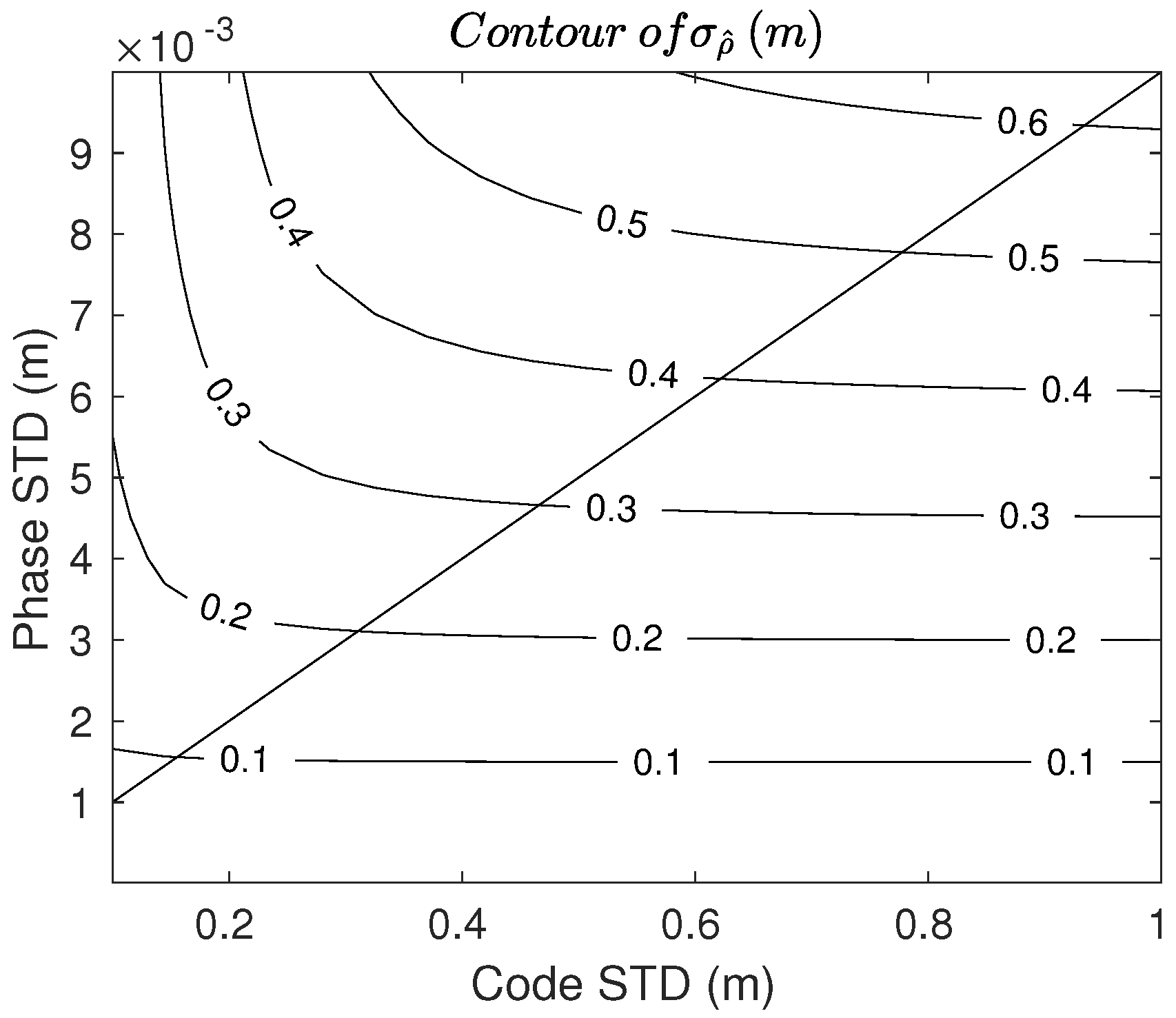
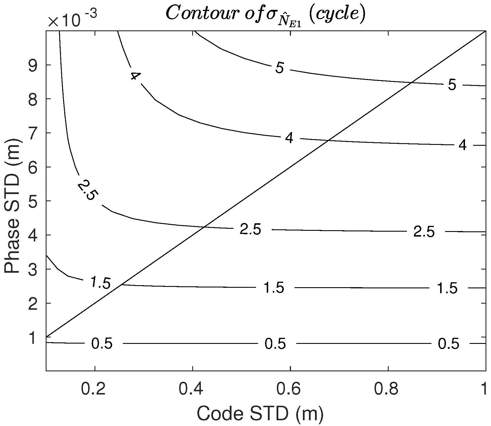
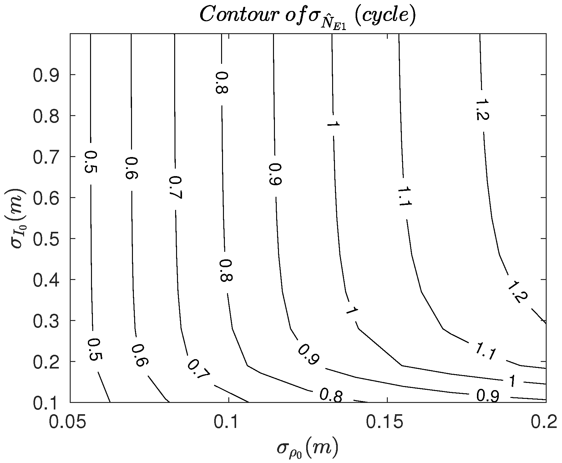
2.2. Stochastic Analysis
3. Experiments and Results
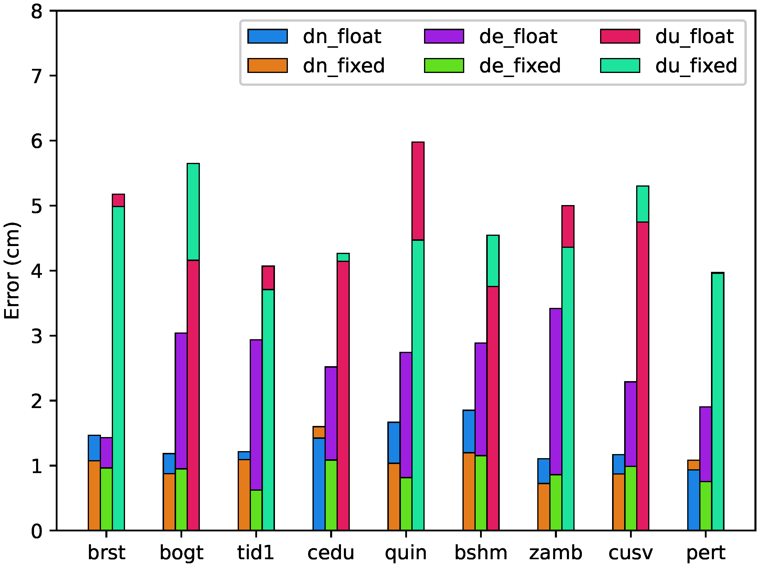
3.1. Multiple-Epoch Filtered Positioning
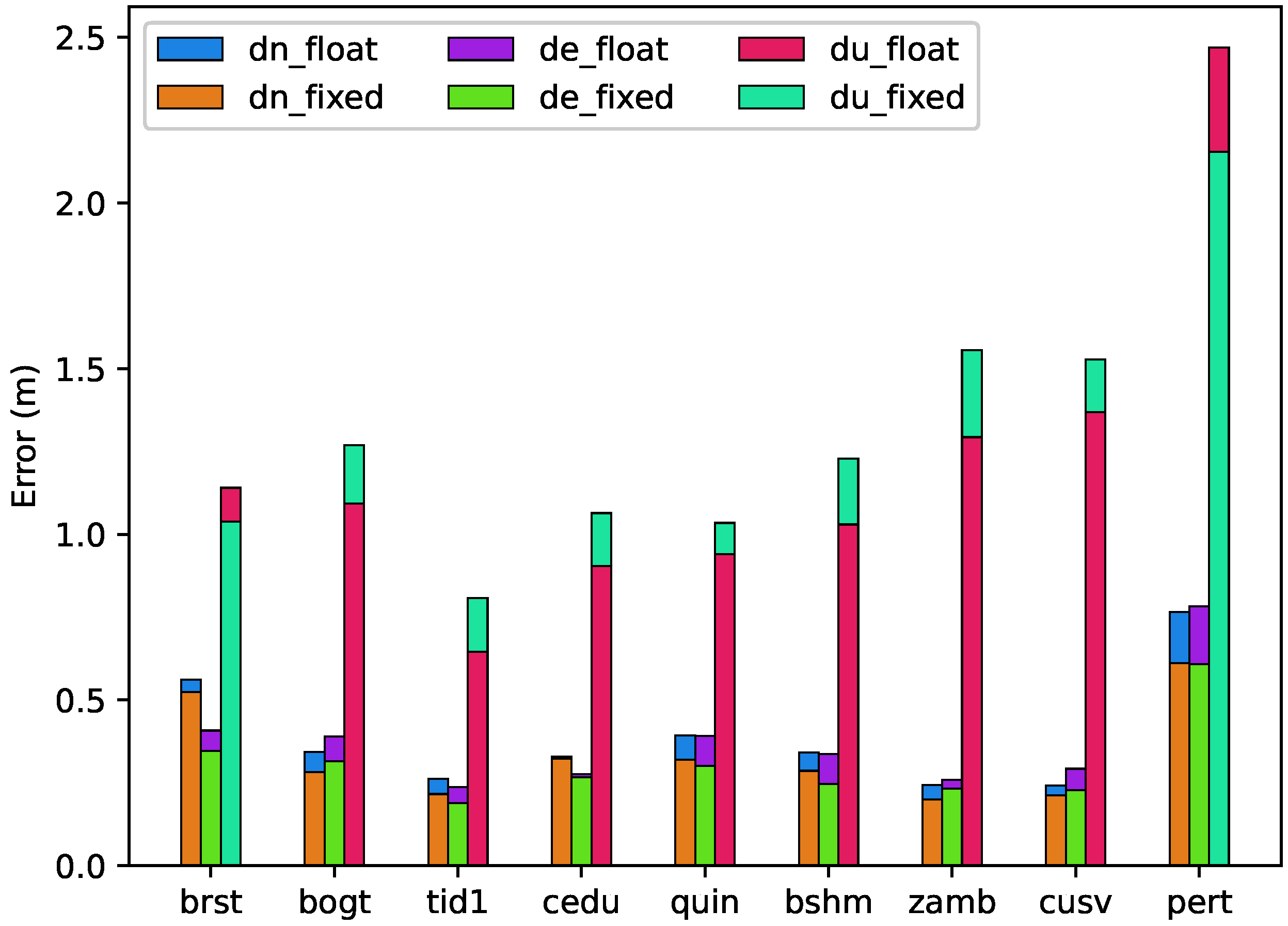
3.2. Single—Epoch Positioning
4. Discussion
5. Conclusions
Author Contributions
Funding
Data Availability Statement
Acknowledgments
Conflicts of Interest
References
- Montenbruck, O.; Hugentobler, U.; Dach, R.; Steigenberger, P.; Hauschild, A. Apparent clock variations of the Block IIF-1 (SVN62) GPS satellite. GPS Solut. 2012, 16, 303–313. [Google Scholar] [CrossRef]
- Pan, L.; Zhang, X.; Li, X.; Liu, J.; Li, X. Characteristics of inter-frequency clock bias for Block IIF satellites and its effect on triple-frequency GPS precise point positioning. GPS Solut. 2017, 21, 811–822. [Google Scholar] [CrossRef]
- Pan, L.; Zhang, X.; Guo, F.; Liu, J. GPS inter-frequency clock bias estimation for both uncombined and ionospheric-free combined triple-frequency precise point positioning. J. Geod. 2019, 93, 473–487. [Google Scholar] [CrossRef]
- Li, P.; Jiang, X.; Zhang, X.; Ge, M.; Schuh, H. GPS + Galileo + BeiDou precise point positioning with triple-frequency ambiguity resolution. GPS Solut. 2020, 24, 78. [Google Scholar] [CrossRef]
- Guo, J.; Geng, J. GPS satellite clock determination in case of inter-frequency clock biases for triple-frequency precise point positioning. J. Geod. 2018, 92, 1133–1142. [Google Scholar] [CrossRef]
- Geng, J.; Guo, J.; Meng, X.; Gao, K. Speeding up PPP ambiguity resolution using triple-frequency GPS/BeiDou/Galileo/QZSS data. J. Geod. 2020, 94, 6. [Google Scholar] [CrossRef] [Green Version]
- Li, X.; Li, X.; Liu, G.; Feng, G.; Yuan, Y.; Zhang, K.; Ren, X. Triple-frequency PPP ambiguity resolution with multi-constellation GNSS: BDS and Galileo. J. Geod. 2019, 93, 1105–1122. [Google Scholar] [CrossRef]
- Li, X.; Liu, G.; Li, X.; Zhou, F.; Feng, G.; Yuan, Y.; Zhang, K. Galileo PPP rapid ambiguity resolution with five-frequency observations. GPS Solut. 2020, 24, 24. [Google Scholar] [CrossRef]
- Ge, M.; Gendt, G.; Rothacher, M.; Shi, C.; Liu, J. Resolution of GPS carrier-phase ambiguities in Precise Point Positioning (PPP) with daily observations. J. Geod. 2008, 82, 389–399. [Google Scholar] [CrossRef]
- Cheng, S.; Wang, J.; Peng, W. Statistical analysis and quality control for GPS fractional cycle bias and integer recovery clock estimation with raw and combined observation models. Adv. Space Res. 2017, 60, 2648–2659. [Google Scholar] [CrossRef]
- Wang, J.; Huang, G.; Yang, Y.; Zhang, Q.; Gao, Y.; Xiao, G. FCB estimation with three different PPP models: Equivalence analysis and experiment tests. GPS Solut. 2019, 23, 93. [Google Scholar] [CrossRef]
- Laurichesse, D.; Mercier, F.; Berthias, J.P.; Broca, P.; Cerri, L. Integer ambiguity resolution on undifferenced GPS phase measurements and its application to PPP and satellite precise orbit determination. Navig. J. Inst. Navig. 2009, 56, 135–149. [Google Scholar] [CrossRef]
- Collins, P.; Bisnath, S.; Lahaye, F.; Héroux, P. Undifferenced GPS Ambiguity Resolution Using the Decoupled Clock Model and Ambiguity Datum Fixing. Navigation 2010, 57, 123–135. [Google Scholar] [CrossRef] [Green Version]
- Katsigianni, G.; Loyer, S.; Perosanz, F. PPP and PPP-AR Kinematic Post-Processed Performance of GPS-Only, Galileo-Only and Multi-GNSS. Remote Sens. 2019, 11, 2477. [Google Scholar] [CrossRef] [Green Version]
- Katsigianni, G.; Perosanz, F.; Loyer, S.; Gupta, M. Galileo millimeter-level kinematic precise point positioning with ambiguity resolution. Earth Planets Space 2019, 71, 76. [Google Scholar] [CrossRef] [Green Version]
- Laurichesse, D. Phase Biases Estimation for Integer Ambiguity Resolution. 2012. Available online: https://igs.bkg.bund.de/root_ftp/NTRIP/documentation/PPP-RTK2012/14_Laurichesse_Denis.pdf (accessed on 29 October 2020).
- Laurichesse, D.; Langley, R. Handling the Biases for Improved Triple-Frequency PPP Convergence. GPS World 2015, 26, 49–54. [Google Scholar]
- Laurichesse, D. Phase Biases for Ambiguity Resolution from an Undifferenced to an Uncombined Formulation. 2014. Available online: http://www.ppp-wizard.net/Articles/WhitePaperL5.pdf (accessed on 1 November 2020).
- Laurichesse, D.; Privat, A. An open-source PPP client implementation for the CNES PPP-WIZARD demonstrator. In Proceedings of the 28th International Technical Meeting of the Satellite Division of the Institute of Navigation, ION GNSS 2015, Tampa, FL, USA, 14–18 September 2015; Volume 4, pp. 2780–2789. [Google Scholar]
- Liu, T.; Jiang, W.; Laurichesse, D.; Chen, H.; Liu, X.; Wang, J. Assessing GPS/Galileo real-time precise point positioning with ambiguity resolution based on phase biases from CNES. Adv. Space Res. 2020, 66, 810–825. [Google Scholar] [CrossRef]
- Duong, V.; Harima, K.; Choy, S.; Laurichesse, D.; Rizos, C. Assessing the performance of multi-frequency GPS, Galileo and BeiDou PPP ambiguity resolution. J. Spat. Sci. 2020, 65, 61–78. [Google Scholar] [CrossRef]
- Laurichesse, D.; Banville, S. Innovation: Instantaneous centimeter-level multi-frequency precise point positioning. GPS World 2018, 2018, 42–47. [Google Scholar]
- Geng, J.; Guo, J. Beyond three frequencies: An extendable model for single-epoch decimeter-level point positioning by exploiting Galileo and BeiDou-3 signals. J. Geod. 2020, 94, 14. [Google Scholar] [CrossRef]
- Melbourne, W. The Case for Ranging in GPS-based Geodetic Systems. In Proceedings of the 1st International Symposium on Precise Positioning with the Global Positioning System, Rockville, MD, USA, 15–19 April 1985; pp. 373–386. [Google Scholar]
- Wübbena, G. Software developments for geodetic positioning with GPS using TI-4100 code and carrier measurements. In Proceedings of the 1st International Symposium on Precise Positioning with the Global Positioning System, Rockville, MD, USA, 15–19 April 1985; pp. 403–412. [Google Scholar]
- Hide, C.; Pinchin, J.; Park, D. Development of a low cost multiple GPS antenna attitude system. In Proceedings of the 20th International Technical Meeting of the Satellite Division of The Institute of Navigation 2007 ION GNSS 2007, Fort Worth, TX, USA, 25–28 September 2007; Volume 1, pp. 88–95. [Google Scholar]
- Blewitt, G. An Automatic Editing Algorithm for GPS data. Geophys. Res. Lett. 1990, 17, 199–202. [Google Scholar] [CrossRef] [Green Version]
- Liu, Z. A new automated cycle slip detection and repair method for a single dual-frequency GPS receiver. J. Geod. 2011, 85, 171–183. [Google Scholar] [CrossRef]
- Banville, S.; Langley, R.B. Mitigating the impact of ionospheric cycle slips in GNSS observations. J. Geod. 2013, 87, 179–193. [Google Scholar] [CrossRef]
- Teunissen, P.J. Theory of integer equivariant estimation with application to GNSS. J. Geod. 2003, 77, 402–410. [Google Scholar] [CrossRef] [Green Version]
- Odolinski, R.; Teunissen, P.J. Best integer equivariant estimation: Performance analysis using real data collected by low-cost, single- and dual-frequency, multi-GNSS receivers for short- to long-baseline RTK positioning. J. Geod. 2020, 94, 91. [Google Scholar] [CrossRef]
- Teunissen, P.J. The least-squares ambiguity decorrelation adjustment: A method for fast GPS integer ambiguity estimation. J. Geod. 1995, 70, 65–82. [Google Scholar] [CrossRef]
- Herrera, A.M.; Suhandri, H.F.; Realini, E.; Reguzzoni, M.; de Lacy, M.C. goGPS: Open-source MATLAB software. GPS Solut. 2016, 20, 595–603. [Google Scholar] [CrossRef]
- Wu, J.T.; Wu, S.C.; Hajj, G.A.; Bertiger, W.I.; Lichten, S.M. Effects of antenna orientation on GPS carrier phase. Manuscr. Geod. 1993, 18, 91–98. [Google Scholar]
- Banville, S.; Geng, J.; Loyer, S.; Schaer, S.; Springer, T.; Strasser, S. On the interoperability of IGS products for precise point positioning with ambiguity resolution. J. Geod. 2020, 94, 10. [Google Scholar] [CrossRef]


| Parameter estimation | Extended Kalman Filter |
| Orbit and clocks | GFZ rapid products |
| Biases | CNES post-processed products |
| Ambiguity resolution | Best integer equivariant (BIE) estimator |
| Elevation cut-off | 7° |
| Elevation weighting function | where is the elevation angle (radian) |
| Antenna PCO/PCV correction | igs14.atx |
| Site displacement | Pole tides and solid earth tides corrections |
| Earth orientation parameters: IERS EOP 14 C04 | |
| (IAU2000A); Solar system body ephemerides: | |
| NASA NAIF SPICE files | |
| Phase windup | [34] |
| Phase cycle slip detection | [28] |
| Troposphere | Saastamoinen model for the hydrostatic delay |
| Niell mapping function | |
| Estimation on the zenith wet delay | |
| Initial variance: 0.5 m; Model noise: 0.005 mm/s | |
| Ionosphere | Estimation of slant ionospheric delay on L1 |
| Higher-order terms are ignored | |
| Initial variance 10 m; Model noise 2 cm/s | |
| Receiver clock offset | Estimated as white noise; Model noise 1000 m/s |
| Additional receiver clock bias | Initial variance 0 m; Model noise 1 mm/s |
| Receiver state | Simulated kinematic; Model noise: 100 m/s for X Y Z |
| Positioning accuracy reference | IGS MGEX coordinate products |
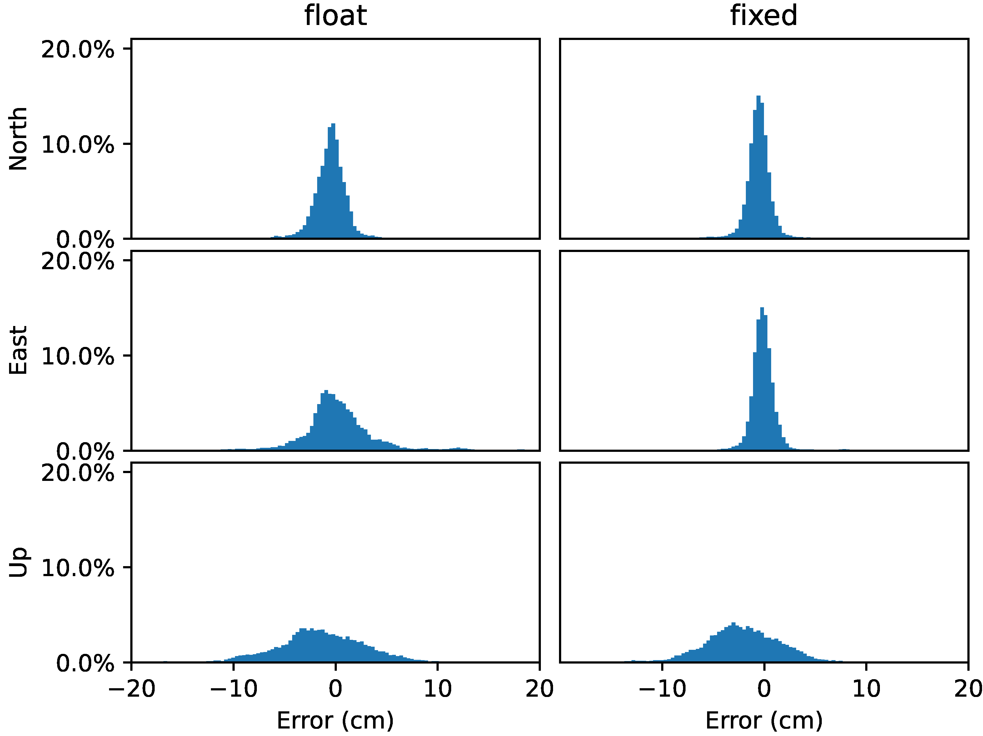
| Model | North | East | Up |
|---|---|---|---|
| Float* | 1.3 | 2.64 | 4.34 |
| Float | 1.37 | 2.63 | 4.48 |
| Fixed | 1.16 | 0.98 | 4.44 |
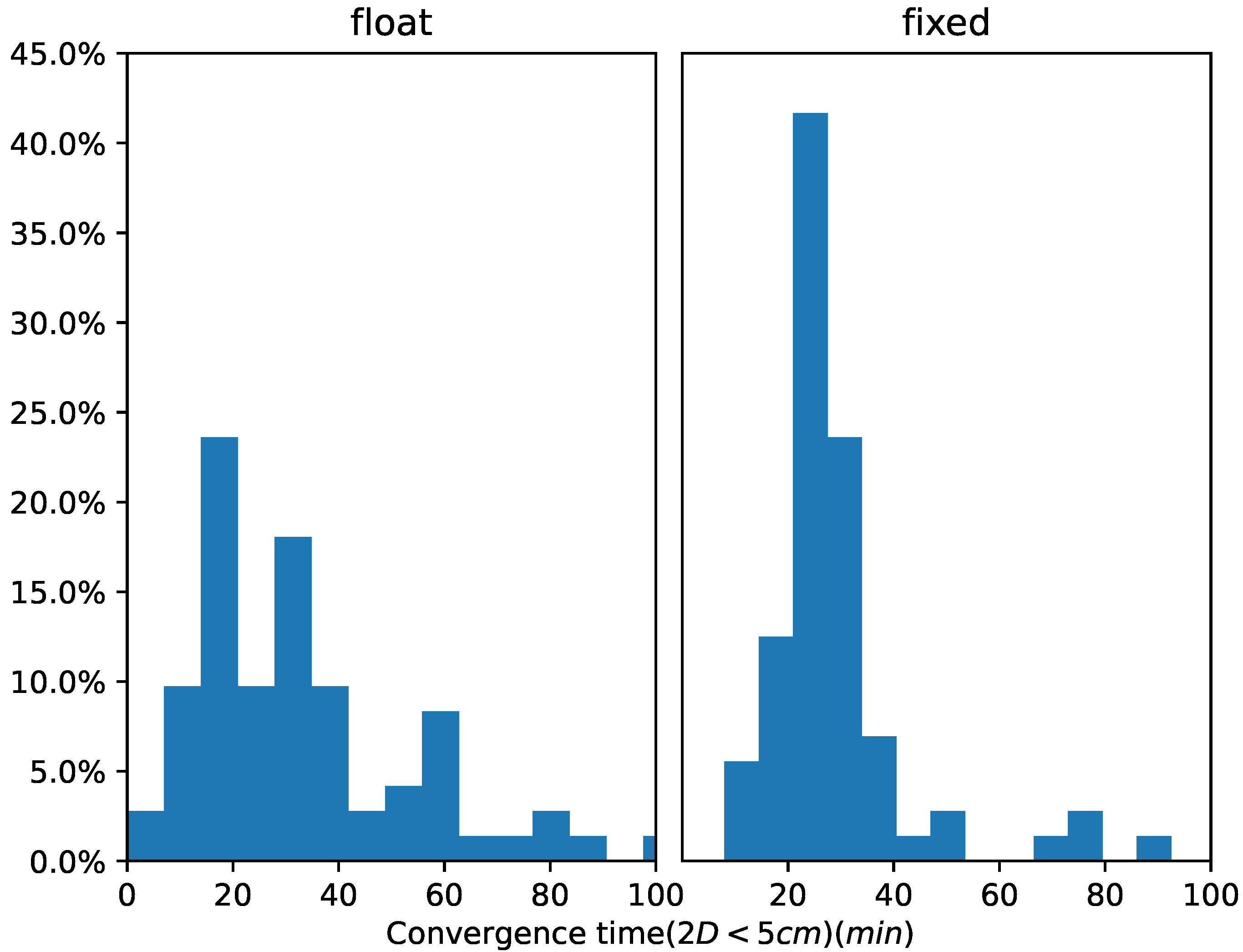
| Float | Fixed | |
|---|---|---|
| Average | 35.1 | 29.2 |
| Std. | 25.3 | 14.4 |
| 68th percentile | 37.1 | 29.6 |
| median | 28 | 25 |
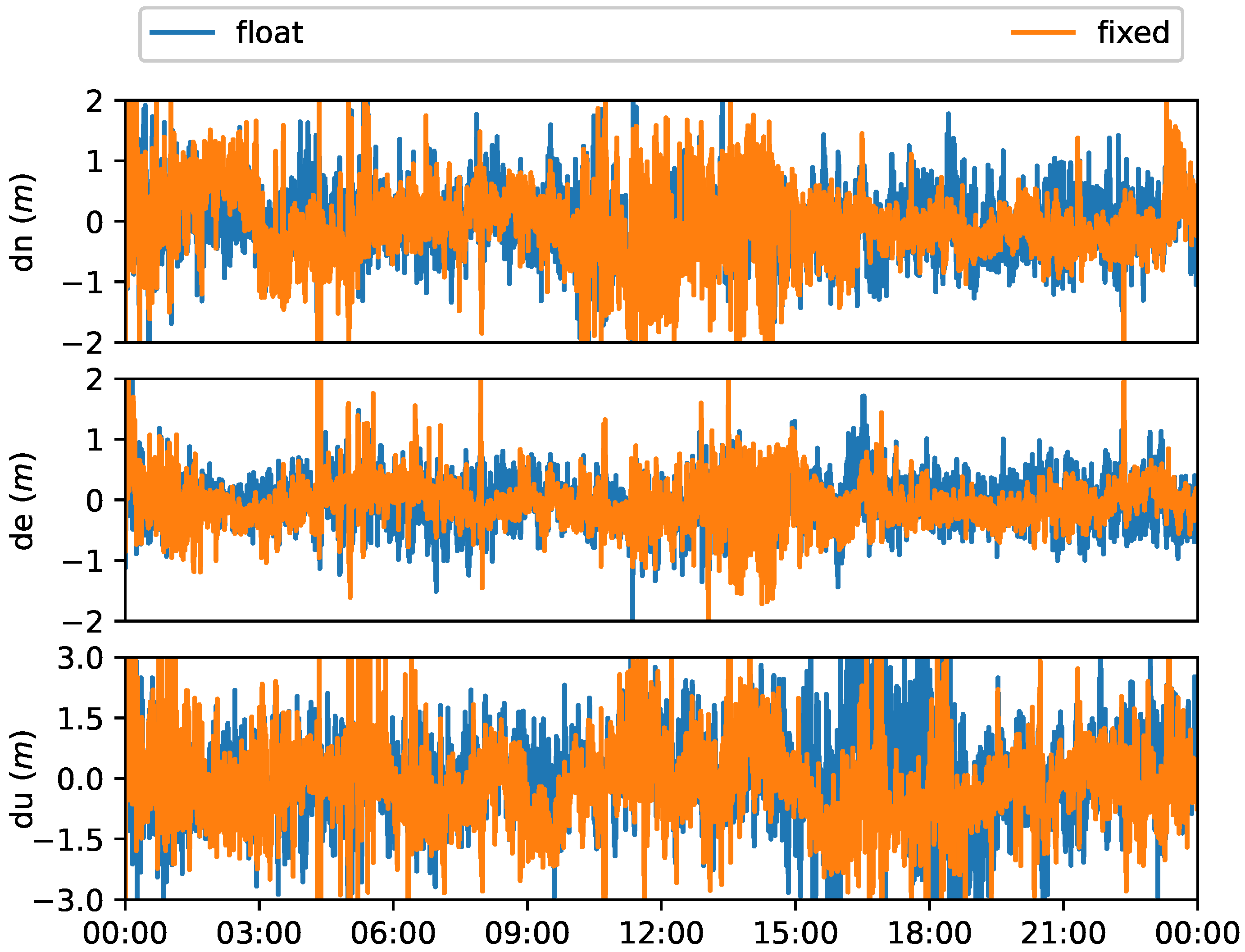
| Model | North | East | Up |
|---|---|---|---|
| Float | 0.37 | 0.37 | 1.11 |
| Fixed | 0.32 | 0.31 | 1.27 |
Publisher’s Note: MDPI stays neutral with regard to jurisdictional claims in published maps and institutional affiliations. |
© 2022 by the authors. Licensee MDPI, Basel, Switzerland. This article is an open access article distributed under the terms and conditions of the Creative Commons Attribution (CC BY) license (https://creativecommons.org/licenses/by/4.0/).
Share and Cite
Zhao, L.; Blunt, P.; Yang, L. Performance Analysis of Zero-Difference GPS L1/L2/L5 and Galileo E1/E5a/E5b/E6 Point Positioning Using CNES Uncombined Bias Products. Remote Sens. 2022, 14, 650. https://doi.org/10.3390/rs14030650
Zhao L, Blunt P, Yang L. Performance Analysis of Zero-Difference GPS L1/L2/L5 and Galileo E1/E5a/E5b/E6 Point Positioning Using CNES Uncombined Bias Products. Remote Sensing. 2022; 14(3):650. https://doi.org/10.3390/rs14030650
Chicago/Turabian StyleZhao, Lei, Paul Blunt, and Lei Yang. 2022. "Performance Analysis of Zero-Difference GPS L1/L2/L5 and Galileo E1/E5a/E5b/E6 Point Positioning Using CNES Uncombined Bias Products" Remote Sensing 14, no. 3: 650. https://doi.org/10.3390/rs14030650
APA StyleZhao, L., Blunt, P., & Yang, L. (2022). Performance Analysis of Zero-Difference GPS L1/L2/L5 and Galileo E1/E5a/E5b/E6 Point Positioning Using CNES Uncombined Bias Products. Remote Sensing, 14(3), 650. https://doi.org/10.3390/rs14030650