Abstract
We address surface wave breaking caused by oceanic Internal Solitary Waves (ISWs) and how ISWs are manifested in the SAR altimeter onboard Sentinel-3A and -3B satellites by means of their effects in Significant Wave Height (SWH). Two different regions of the ocean are selected, namely the tropical Atlantic Ocean off the Amazon shelf and the Banda Sea in the Indian Ocean, where there are scenes of Sentinel-3 OLCI acquired simultaneously with an along-track SAR mode altimeter, which include signatures of large amplitude ISWs. New data of unfocused SAR (UF-SAR 20 Hz) and fully focused SAR (FF-SAR 160 Hz) modes are analyzed, which are retracked in full range and over a reduced range of bins (truncation carried out dynamically ten gates away from the estimated epoch position). At first order, in scales of 1–3 km, a strong decrease in the normalized radar cross section (NRCS) over the rough part of the ISWs is observed followed by a small increase in the smooth part relative to the unperturbed ocean background. A second order ISW signature, in scales of 20 km, is noted: the SWH is attenuated after the passage of an ISW, considering length scales of about 10 km before and after the ISW crest. The SWH signatures are unique in showing that the surface wave energy does not return to its unperturbed level after the passage of an ISW, admittedly because intense meter-scale wave breaking results in surface wave energy dissipation. Furthermore, Sentinel-2 MSI images are analyzed and provide insights into this same phenomenon: white-capping resulting in a radiance increase at all (visible) wavelengths. Modulation of breaking waves owing to ISWs is demonstrated by estimates of the fraction of breaking waves in the presence of internal waves.
1. Introduction
1.1. Oceanic Internal Waves, Their Surface Manifestations and Remote Sensing
Oceanic internal waves are waves propagating in the interior of the ocean, usually along density interfaces such as the seasonal or permanent pycnocline. They are allowed to propagate when the ocean consists of layers of different densities, i.e., when the ocean is stratified, and when there is a physical mechanism that can perturb the interface between the layers, which, in coastal areas, is most often tidal flow over shallow bottom topography gradients. In most cases, the internal waves are nonlinear and appear in wave packets consisting of several internal solitons and are hence often called Internal Solitary Waves (ISWs). We will adopt this terminology throughout this paper. The ISWs become detectable from space primarily via ISW-induced variation of the sea surface roughness, which is detectable by optical and radar sensors, and in particular by Synthetic Aperture Radars (SARs). Historically, ISWs have first been detected from space on photographs taken by astronauts, who have pointed their hand-held cameras into the sunglint region. The sunglint region is the sea surface area from which the sunlight is reflected at roughly the same angle as the camera is viewing the surface. Since 1972, ISWs have also been detected on sunglint images taken from satellites, such as the American Landsat-1, which was called at that time the Earth Resources Technology Satellite [1]. However, optical images have their limitations in ISW studies, since they can be taken only during daytime when the sky is cloud-free or almost cloud-free and when certain criteria concerning the viewing geometry are fulfilled.
A breakthrough in ISW remote sensing from space came with the launch of the American Seasat satellite in 1978. The L-band (1.25 GHz) SAR on this satellite captured numerous ISWs [2,3,4]. Since then, many more ISW images have been acquired from various satellites, such as the European ERS-1/ERS-2, Envisat, and Sentinel-1A/1B satellites, the Canadian Radarsat-1/2 satellites, the Japanese ALOS satellite, and the Chinese Gaofen-3 satellite. ISW sea surface signatures have also occasionally been detected in ocean color images [5,6] and recently also in radar altimeter data [6,7,8,9,10].
There are two fundamentally different radar-based sensors operating from orbiting satellites; they are side-looking imaging SARs, which look down at an oblique angle to the side of the satellite orbit, and nadir-looking instruments that are pointed directly down towards the Earth. Despite the fact that both types of sensors are active instruments, meaning that they emit their own microwave pulses and record the subsequent echoes, their data acquisition geometries are intrinsically different, and they survey different aspects of ocean dynamics.
On the one hand, imaging SARs are sensors which acquire two-dimensional measurements of the ocean’s horizontal surface. They comprise very high spatial resolutions (up to the order of meters), in which backscattered radiation returning into the satellite direction is described, to a first order, by a Bragg scattering mechanism. Bragg scattering is particularly successful to account for sea surface signatures of small-scale phenomena via their changes in sea surface roughness mainly induced by wind wave and surface current variability. On the other hand, satellite altimeters are not imaging sensors. The recorded echoes are registered along a single “line” corresponding to the satellite’s ground-track, and hence their data are usually referred to as along-track data. This “line” corresponds to the satellite’s flight direction (or azimuth) projected onto the earth’s surface, and nominal spatial resolutions are of the order of kilometers—although new generation altimeters can reduce this to a few hundred meters in the along-track direction.
Nonetheless, both radar-based sensors use microwaves as their sensing radiation. This means using wavelengths of the order of centimeters (e.g., Ku and C bands have nominal wavelengths of about 2 and 4 cm, respectively), which in turn interact with similar length scales of the sea surface (note that the sea surface is essentially opaque to microwaves). Therefore—to leading order—they are essentially sensitive to centimeter-scale waves, which are mostly wind-generated in the ocean and hence (in practice) an intrinsic feature of the sea surface. It is well known that wind waves will naturally interact and group in progressively larger waves (see e.g., [11]). When wind waves are continuously fetched by the sea surface (i.e., assuming there is at least a mild wind), these growing waves will continue to increase in amplitude until some equilibrium balance is reached—upon which they eventually break, and their energy (which had been accumulating from the wind) dissipates. This brings about an important question: Since breaking surface waves are an inherent part of the ocean wave field, how do they affect the radar signature of other oceanic phenomena, such as oceanic fronts, oceanic eddies, and internal waves?
In principle, isolating the contributions owing to surface breaking waves from other potential contributions could be beneficial for understanding and quantifying different radar backscattering mechanisms. This can be achieved by having a nominal background (i.e., sea surface unperturbed by current shears and wind variability) against which two contrasting sea surfaces could be compared: one having little (or no) surface breaking waves, and another having a significant amount of enhanced surface wave breaking. Furthermore, the corresponding horizontal scales should be sufficiently large to ensure distinct transitions in the remotely sensed radar ground footprints—preferably located in deep ocean conditions and away from the more dynamical coastal environments. Interestingly, these exact conditions can be naturally found in deep ocean conditions, e.g., in the Tropical Atlantic Ocean off the Amazon River mouth. Consequently, large-amplitude ISWs with horizontal wavelength scales around 1 to 10 km and crest lengths of more than 100 km, which typically include a rougher leading section (often with patches of enhanced surface breaking and whitecaps) and a smooth (slick-like) trailing section, are ideally suited to investigate enhanced surface wave breaking contributions to both satellite SAR altimeters and imaging sensors.
The paper is organized as follows: in Section 1.2, we address wave breaking in the context of ISWs’ manifestations, e.g., quoting from a report written in the 19th century in which mariners describe observations of roughness bands in the Andaman Sea, which must have been sea surface signatures of strong ISWs, and then we present a typical photograph taken from a ship which shows sea surface signatures of ISWs containing breaking surface waves. All the data and methods used in this work are described in Section 2. In Section 3, we present new observations from SAR altimetry (from the Sentinel-3 mission) with clear evidence of Significant Wave Height (SWH) variations along the propagation paths of ISWs in scales of about 20 km or more. New advanced SAR altimetry products (e.g., Fully Focused FFSAR) are presented and compared with standard Copernicus products. Evidence of wave breaking in high-resolution optical images owing to large ISWs is also presented in Section 3. Finally, in Section 4, we summarize our results and conclusions.
1.2. Surface Wave Breaking Induced by Strong ISWs
Wave breaking is a ubiquitous phenomenon in the ocean at high to medium wind speeds. It generates turbulence in the upper ocean layer and causes dissipation of wave energy. However, ocean surface waves can break also in the absence of wind, for instance when a swell shoals on a beach. This paper deals with breaking surface waves, which are not generated by the action of the wind, but by a resonant interaction with an ISW as will be discussed later in this section.
There are numerous visual observations, in particular from ships, that ISWs are associated with bands of choppy waters containing surface breaking waves. An early description of this phenomenon can be found in the book of Maury [12], which is quoted in Osborne and Burch [13]. This book contains reports about roughness bands or ripplings, which are often observed from ships in the Andaman Sea: “The ripplings are seen in calm weather approaching from a distance, and in the night their noise is heard a considerable time before they come near. They beat against the sides of a ship with great violence, and pass on, the spray sometimes coming on deck; and a small boat could not always resist the turbulence”. “The ripplings consist of broken water, which makes a great noise when the ship is passing through the ripplings in the night”. At that time, it was not known that the roughness bands are sea surface manifestations of ISWs. However, Perry and Schimke [14], who made oceanographic surveys in the Andaman Sea north of Sumatra from a ship in 1964, identified the roughness bands or “rips” as sea surface signatures of “large-amplitude internal waves”. They observed roughness bands, which ranged from 200 to 800 m in width, stretched from horizon to horizon (approximately 30 km), and had a spacing of about 3200 m between the bands. The bands of choppy water contained short, steep, randomly oriented waves with heights of about 0.3 to 0.6 m. Each band stood out distinctly in an otherwise undisturbed sea (wind speed: 4 m/s). Moreover, Osborne and Burch [13] observed roughness bands in the Andaman Sea during a campaign, which was designed to measure internal waves and the associated response of a drillship simultaneously, and attributed them to sea surface manifestations of ISWs. On one occasion, they observed six distinct roughness bands, each approximately 600 to 1200 m wide, with breaking waves about 1.8 m high. After the passage of the roughness band, the wave heights quickly decreased in wave height to less than 0.1 m, and the sea surface had the appearance of a “millpond”. The entire process repeated at approximately 40 min intervals.
Enhanced surface wave breaking associated with large-scale ISWs is now widely accepted, and in Figure 1 we present a photograph taken from Research Vessel (R/V) Charles Darwin in the central region of the Bay of Biscay (approximately 46°N, 7°W), in which a band of strongly increased sea surface roughness containing surface breaking waves is visible. It is associated with a large-amplitude internal wave generated by a tidal internal wave beam in deep water [15]. It seems that the breaking waves have wavelengths in the order of meters. In these large-scale ISWs (with horizontal scales of the order of kilometers), enhanced effects in surface wave breaking may be imaged in high spatial resolution satellite images. Figure 2 shows an image taken in the visible band by the Multispectral Instrument (MSI) onboard the Sentinel-2A satellite (resolution: 10 m) showing also sea surface signatures of an internal wave packet in the Banda Sea (in the Indonesian Seas) generated over a sill in the Ombai Strait in between the Alor and Atauro Islands, one of the major passages of the Indonesian Through Flow. In this case, whitecaps are visible (Figure 2c, and respective inset to the right) which are generated by breaking waves associated with the internal wave.
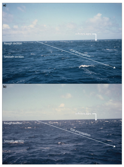
Figure 1.
Photographs taken from the Research Vessel Charles Darwin showing sea surface manifestations of a large-amplitude ISW advancing towards the ship in the central region of the Bay of Biscay, which includes surface wave breaking (i.e., whitecaps). Note that both panels (a,b) are just a few minutes apart, and wave breaking has moved towards the ship from (a) to (b). Courtesy: Adrian L. New from the National Oceanography Centre, Southampton.
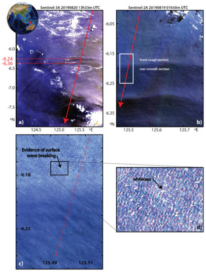
Figure 2.
(a) Quasi-true color image (Level-1b) acquired on 20 August 2019 at 13 h 33 m UTC by the OLCI sensor onboard the Sentinel-3A satellite (see inset for location). The red line represents the ground-track of the satellite, which in this case is close to the ISWs’ direction of propagation. (b) Image taken in the visible band by the Multispectral Instrument (MSI) onboard the Sentinel-2A satellite on 19 August 2019 at 01:50 UTC showing sea surface signatures of an ISW packet. Note the bright spots aligned in bands, which are evidence of whitecaps generated by breaking surface waves. The red line represents the ground-track of the satellite Sentinel-3, approximately one day after. (c) Zoom of the Sentinel-2 image in (b), in the location of the white rectangle. A larger zoom is also displayed in (d), representing the black rectangle in full resolution, and showing whitecaps.
As stated before, we attribute the roughness bands associated with ISWs as caused by a resonant interaction between surface waves and the internal waves. Such an interaction has been studied theoretically (see e.g., [16,17,18,19,20]) and was verified in laboratory experiments [17,19]. Resonance occurs when the group velocity of the surface waves (cgroupsw) matches the phase speed of the internal waves (cphaseiw):
cgroupsw = cphaseiw
While Lewis et al. [17] studied this interaction for a monochromatic internal wave, Kodaira et al. [19] studied it for an ISW, although in laboratory conditions, their results strictly refer to capillary surface waves, and hence their findings may not directly apply to resonance with meter-scale surface waves. The slowly varying surface currents associated with the ISW interact with the surface waves, and those waves which are in resonance or near-resonance with the varying surface current field steepen and give rise to the appearance of short-wave packets on the sea surface. According to the theory of Kodaira et al. [19], the wave packet is located above the front half of the ISW and propagates with a speed close to that of the ISW underneath, which is in agreement with observations. Applying Equation (1) and using the dispersion relation for deep water waves, the resonant surface wave has a wavelength of:
λresonantsw = (8π/g) (cphaseiw)2
For a typical phase speed of 2 m/s for an ISW, we obtain λresonantsw = 10 m, which is a typical wavelength of an “intermediate-scale wave”. It has long been suspected that these waves are strongly modulated by internal waves [21,22], and that their breaking on the sea surface contributes to the high radar backscatter signatures of internal waves. When these surface waves break, they generate turbulence in the upper surface layers and dissipate energy. The breaking stage is maintained by a replenishment of energy from the ISW via the resonant interaction. It is often assumed that surface wave breaking occurs when the phase velocity equals the orbital velocity of the wave, which results in H ≥ λ/2π, where H is the surface wave height, and λ its wavelength. However, Ochi and Tsai [23] propose the condition H ≥ 0.020gT2, where g is the acceleration due to gravity, and T the surface wave period, which results from laboratory measurements with random waves. In terms of wavelength, the condition reads:
H ≥ 0.142 λsw
Note that Equation (3) is consistent with the Stokes [24] criterion for surface breaking waves. Therefore, for a typical wavelength λsw of 10 m, we obtain for the height of the breaking surface wave H = 1.5 m. Wave heights of this order, but slightly larger (1.8 m), have been measured in roughness bands associated with an ISW in the Andaman Sea by Osborne and Burch [13], where the speed of the ISW was 2.2 m/s, and thus the wavelength of the resonating surface wave λresonantsw = 12.4 m (which would yield H = 1.76 m). As will be shown in Section 3, we obtained similar values in our analysis of Sentinel-3 altimetry data.
2. Materials and Methods
In previous work, it was discussed how surface wave breaking (resulting from ISWs) is thought to affect the radar backscatter in imaging SARs (see e.g., [10,25]). Since SAR altimeters, with enhanced spatial resolution, also use active microwaves to sense surface roughness, it is reasonable to assume that surface wave breaking will make a measurable signature in their radar returned echoes—even though they have a different nadir-looking acquisition geometry and operate in the more energetic part of the microwave spectra.
2.1. Fundamentals of Satellite Altimetry and Its Sea Surface Signatures of ISWs
Before proceeding to investigate possible contributions from surface wave breaking in satellite altimeters, it is important to explain the fundamentals of satellite altimetry and the mechanisms that allow it to detect the sea surface manifestations of ISWs. In essence, satellite altimeters use nadir-pointed radar pulses (i.e., microwave pulses emitted directly downwards in the vertical from the satellite) to “illuminate” the sea surface and record their subsequent microwave echoes. The altimeter echoes are recorded along the satellite’s flight (or azimuth or along-track) direction, meaning data are recorded and related to a single footprint on the ground, and along one-dimensional paths (i.e., the satellite’s ground-track) rather than in a two-dimensional image format.
The primary and most traditional measurement made by an altimeter is the two-way travel time from radar echoes received from the backscatter radiation, which of course translates to a distance after a series of very accurate corrections in microwave propagation speeds are accounted for along the two-way traveled distance through the Earth’s atmosphere. These distances can then be referenced to a mean sea level to yield e.g., the well-known Sea Level Anomalies (SLAs) or sea level height anomalies, once the marine geoid is used.
The altimeter’s echoes that are reflected backwards to the satellite antenna are recorded onboard over a period of time, meaning that not only times but also the power and shapes of the backscattered radar intensities can be used to estimate geophysical properties of the sea surface. These echoes are usually termed waveforms, and each waveform corresponds to an emitted pulse which returns to the sensor after reflection at the sea surface. For the ocean, surface waveforms typically follow a well-known pattern. An illustrative example is shown in Figure 3a, which is seen to begin at the sensor’s noise floor (preceding the echo’s arrival, also denominated thermal noise), then raising rapidly as the emitted pulse returns to the sensor (often termed the waveform’s leading slope), and finally decreasing along a trailing edge. Well-established algorithms (called retracking algorithms) are used to fit the recorded waveforms to those expected from theory and hence provide estimates for several geophysical quantities that are typically used in ocean sciences [26,27]. The Normalized Radar Cross Section (NRSC), which is a measure of the power received in the radar backscatter, depends mostly on the small-scale sea surface roughness (about three times the radar wavelength, i.e., greater than about 7 cm for Ku-Band), and relates closely to the waveforms’ maximum power. The Significant Wave Height (SWH), which is a statistical measure of the highest third waves of the local wave spectrum, relates to the waveforms’ leading slopes (see Figure 3a).
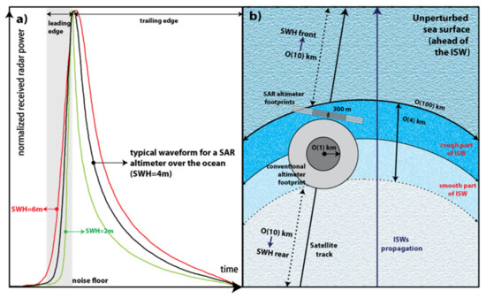
Figure 3.
(a) Normalized SAR altimeter waveforms for an unperturbed (in relation to the ISWs’ surface manifestations) sea surface (black) and for different SWHs (green and red). (b) Schematic representation of a typical ISW and footprints of a conventional (circular shape) and a SAR altimeter (SRAL, rectangular shapes). Dark gray represents illuminated areas corresponding to maximum backscattered power, and light gray the decaying part of the echo due to off-axis antenna gain attenuation.
It is well known that Internal Tides (ITs, i.e., IWs of tidal period with horizontal length scales of order of tens to hundreds of kilometers) can be successfully mapped using sea surface height data from satellite altimeters (see e.g., [28]). Magalhaes and da Silva [7] showed that conventional satellite altimetry can also detect the sea surface roughness signatures of large-scale ISWs (i.e., with horizontal scales of about 10 km), in which the waveforms were found to change significantly. In particular, the high-sampling rate (20 Hz) of the Jason-2/3 altimeters made it possible to detect several short-period signatures in the NRCS (or σ0) data, which resulted from ISWs.
2.2. Sentinel-3 SAR Altimeter and Detection of ISWs
New generation satellite altimeters, which use SAR processing in the along-track direction to simulate larger antenna apertures, increase the along-track ground resolution. They are commonly known as SAR altimeters (e.g., those flying onboard ESA’s Cryosat-2 and Sentinel-3 missions and more recently on the Copernicus Sentinel-6 Michael Freilich satellite). Nonetheless, this SAR processing, which uses the echoes’ Doppler Effect induced by the satellite motion, can only be used in the sensor’s direction of flight—i.e., in the along-track direction. This means that, in practice, the ground resolutions of these more advanced altimeters are in fact sharpened to about 300 m in the along-track direction (nominal along-track resolution), but still remain the same as those of conventional altimeters in the across-track direction (i.e., more than 1 km as illustrated in Figure 3b).
The reduced along-track footprint of SAR (or Delay/Doppler) altimeters relative to conventional altimeters is achieved through a technique developed in the 1990s (see [29]), by which return radar echoes are recorded in both range bins (time domain) and the Doppler frequency shift. Although the reflections from direct nadir have no Doppler shift, those reflections from a little in front of the sub-satellite point are shifted to a slightly higher frequency and those behind to a lower frequency. This is made possible thanks to the SAR altimeter capability of operating at a high pulse repetition frequency (PRF) (at a higher rate than conventional altimeters) which ensures the needed “pulse-to-pulse” radar waves coherence for delay/Doppler signal processing.
Depending on how ISWs crests are oriented relative to the altimeter ground track, this means that the altimeter’s footprint (i.e., the area of the illuminated sea surface) will be distributed differently between the unperturbed background (i.e., unaffected by ISWs) and the ISWs’ sea surface manifestation patterns (as shown in Figure 3b). Note that individual waveforms can come from just one of these characteristic footprints, which may or may not exhibit strong contrasts relative to the unperturbed background according to the orientation of the sharpened along-track footprint in relation to the ISW crests and troughs. If the sharpened along-track direction of the satellite is aligned with the waves’ direction of propagation, it is likely that large-scale ISWs produce a clear signature in the SAR radar altimeter. This is the case shown in Section 3 for the Banda Sea, and to some extent is also the case for the Tropical Atlantic Ocean cases shown in this paper.
Santos-Ferreira et al. [8,9] already documented how the sea surface roughness signatures of large-scale ISWs can affect the enhanced resolution waveforms in SAR altimeters. They used optical imagery from Sentinel-3 (from the Ocean and Land Color Instrument—OLCI) to inspect and validate visually the sea surface manifestations of ISWs that could be unambiguously identified (in synergy) with the SAR altimeter data, which are acquired simultaneously from the SAR altimeter (i.e., the SRAL) onboard the Sentinel-3 satellites. It was shown that the SRAL footprint is small enough (about 300 m in the along-track direction), and it can capture radar power fluctuations over consecutive ISW crests and troughs, and hence over rough and slick surface patterns arrayed in parallel bands with scales of a few kilometers.
The morphology of SAR waveforms is also significantly altered in the presence of ISWs—including SWH estimates, since the leading slopes (in SAR waveforms) feature a variable steepness between the internal waves’ leading and trailing sections (see Figure 3 and Figure 4 in [8]). This feature is relevant in the framework of this paper because SAR waveforms are sensitive to SWH along an ISW section (crest and trough), and appear to be sensitive to enhanced surface waves within a given signature of ISWs. Hence, re-tracked geophysical parameters such as σ0 or SWH are suited to investigate possible contributions in the altimetry echoes resulting from enhanced surface wave breaking.
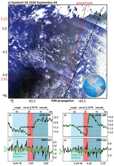
Figure 4.
(a) Quasi-true color image (Level-1b) acquired on 4 September 2020 at 13h01m UTC by the OLCI sensor onboard the Sentinel-3B satellite (see inset for location). The red line represents the ground-track of the satellite, which in this case is practically parallel to the ISWs’ direction of propagation. (b) Along-track 20 Hz NRCS (i.e., σ0) measured by the SRAL altimeter showing variations of approximately 2 dB in the leading ISW around 3.95°N. (c) SWH 20 Hz for the same ISW showing a larger-scale variation of 0.53 m when comparing the section in front of the leading wave with that in the rear. (d) Same as (b) for the leading ISW around 5.22°N, with variations of approximately 3 dB (e) Same as (c) showing a larger-scale variation of 0.35 m.
2.2.1. Sentinel-3 Unfocused SAR (UFSAR)
In this paper, we explore the radar altimeter system on board Sentinel-3 satellites in the unfocused SAR mode (UFSAR) and Fully Focused SAR mode (FFSAR) over the open ocean. This system is composed by the SAR Radar Altimeter (SRAL) together with the MicroWave Radiometer (MWR) and Precise Orbit Determination (POD) sub-systems for ocean topography measurements.
As implemented in the Sentinel-3 mission, the SRAL emits patterns of 64 coherent Ku-band (13.575 GHz, bandwidth = 320 MHz used) pulses in (closed) bursts at a PRF of approximately 18 kHz, enclosed by two C-band (5.41 GHz, bandwidth = 290 MHz used) pulses to provide an ionospheric bias correction (see e.g., [30,31]). The SAR altimetry processing first consists of coherently combining pulses from a burst to generate Doppler beams that are further steered to different surface samples’ location on the ground. A set of Doppler echoes originating from different bursts are then gathered at each surface sample (typically 212 looks) to form a stack that can subsequently be incoherently averaged to produce a multi-looked echo (also termed SAR-mode echo) with a much higher signal-to-noise ratio (see [31], and references therein for more details). The multi-looked echo has a beam-limited illumination pattern in the along-track direction while maintaining the pulse-limited form in the across-track direction. Hence, a sharpened along-track spatial resolution (around 300 m for Sentinel-3 SRAL) is achieved whereas in the across-track direction, it is still limited to the diameter of the pulse-limited circle (see Figure 3b). A mean least square estimator (retracking algorithm denominated SAMOSA, see [32] for details) is adjusted to each multi-looked echo, and hence it is possible to retrieve geophysical parameters such as range, SWH, and σ0 that are inferred from the amplitude of the fitted waveform. The shape of the multi-looked echo has a steeper leading edge than waveforms from conventional radar altimeters, and thus the range is determined more precisely (within less than 1.3 cm at 2 m SWH in SAR mode on board Sentinel-3, see [33]).
Sentinel-3 SRAL Non-Time-Critical (NTC) Marine Level 2 products are used in the first part of this study. The data are distributed by EUMETSAT through Copernicus Online Data services (http://archive.eumetsat.int/usc/, accessed on 27 April 2021). The product contains “enhanced measurement” data files which include radar waveforms corrected for Automatic Gain Control (AGC), Sea Level Anomaly (SLA), SWH, σ0, and other auxiliary variables at 20 Hz. Wind speed at 10 m height (U10) is provided in this product at 1 Hz.
2.2.2. Sentinel-3 Fully Focused SAR (FFSAR)
The fully focused SAR technique is a novel altimetry approach inherited from SAR imagery systems which, unlike SAR mode processing, optimizes the focusing of the radar pulses along the satellite ground track to achieve the highest possible resolution in azimuth. The FFSAR concept was originally designed for altimetry by Egido and Smith [34] and first used with Cryosat-2 data demonstrating its improvement over UFSAR data on many water surfaces. The focusing technique consists of a coherent combination of the pulse echoes that are acquired over the illumination time of a scatterer on the surface. This processing involves a fine alignment of the echoes in the phase and range to make them coherent to focus on the point target, then a summation to produce a single-looked waveform at that position with the highest along-track resolution (up to 50 cm corresponding to the theoretical limit of half the antenna length). Successive singled-look echoes are thereby generated along the track, spaced approximately 40 cm apart according to the pulse repetition interval. This unprecedented gain in resolution is of particular interest for probing water surfaces within highly heterogeneous scenes such as inland waters, sea-ice leads, and coastal areas. Over rough homogeneous surfaces such as the ocean, the speckle noise is particularly present in the backscattered signal, which masks any low-amplitude signals. Consecutive singled-look echoes are thus summed incoherently to reduce the speckle and form a (less-noisy) multi-looked waveform, at the expense, however, of a loss in resolution. The number Nsl of single looks that are summed into one multi-looked waveform gives the posting rate P in Hz, defined as . The noise reduction brought by the FFSAR multi-looking is much more effective than for the unfocused SAR methods [34], allowing higher along-track resolution to be used, while ensuring high precision altimeter measurements. The present study seeks to exploit such potential FFSAR improvements to resolve small-scale sea surface features better such as ISWs, that conventional altimetry fails to capture adequately. In this respect, FFSAR data were processed at a 160 Hz posting rate (equivalent to a 40 m spacing between measurements on ground) then assessed to determine whether ISW-induced signals can benefit from higher sampling rates.
Despite this improvement, one should note that the lacunar sampling of the Sentinel-3 closed-bursts chronogram introduces replicas in the azimuth FFSAR point target response (PTR), which alters its along-track resolution [34]. This makes it difficult to separate real scatterers’ signal from replicas once they are superposed. However, for long wavelength waves of a few kilometers such as ISWs, the impact of the replicas’ contamination coming from forward or backward waves might not be that important since replicas appear every 90 m on average and rapidly fall off in amplitude for increasing range.
Besides that, it was shown that the orbital wave velocities are widening the azimuth point target response of the UFSAR and more particularly the FFSAR processing [35,36], resulting in the degradation of their native along-track resolution. This further leads to a SWH over-estimation (about 10–15 cm at maximum) if the SAR altimeter retracking model does not account for this sea-state parameter.
2.2.3. Retracking of SAR Altimeter Waveforms
Geophysical parameters are estimated from Sentinel-3 FFSAR 160-Hz and UFSAR 20-Hz waveforms, generated over the Banda Sea and Tropical West Atlantic areas, using a common retracking algorithm. The retracking consists of fitting at best (in an optimization sense) the altimeter waveforms with a model dependent on geophysical parameters determined here by Levenberg–Marquardt optimization. In the SAR mode, the ocean retracking model was analytically formulated by Ray et al. [32] translating the conventional altimetry Brown model (see [26]) to SAR altimetry. This model expressed in the time domain is based on the convolution of three terms (probability density function, impulse response function, and the flat sea surface response) which is quite time-consuming. A faster computational approach replacing the time domain convolution by the frequential domain multiplication was introduced by Buchhaupt [37].
A similar frequential model retracking algorithm as the one developed in Buchhaupt [37], called SARmultilookLS3, was used in this study estimating the classical ocean parameters as the range, SWH, and σ0. One fundamental assumption of the associated waveform model is that of considering a constant backscattering over the total area illuminated by the radar. However, this assumption is not always valid, depending on the sea surface roughness that is present within the altimeter footprint. One way to improve the model is to introduce a mean square slope (mss) parameter, to account for the dependency of σ0 with respect to the viewing angle, using the geometrical optics theory as it is conducted in some published works (see [38,39]). Such an adaptive retracking algorithm that additionally estimates a constant mss was developed and applied in this study. It is called SARmultilookLS3_MSS, abbreviated as MSS throughout the rest of the paper.
Another possible source of error in the waveform modeling is the σ0 heterogeneity that is characteristic of ISWs (where high and low values are observed on different sides of the radar footprint of the same ISW front). This is particularly the case when the wave does not propagate in the same direction as the satellite track, resulting in variations of the mss within the radar footprint (that is not accounted for in the model) and potentially leading to biases on the geophysical parameters. To mitigate these errors, a proposed solution is to reduce the range window used in the retracking, i.e., estimate the parameters only on a portion of the waveform around the leading edge. The altimeter footprint size is in turn reduced in the cross-track direction, making the constant mss assumption more likely to be valid, at the expense, however, of an increase in the measurement noise. Based on that, two different approaches were considered: one using the full range of the waveforms as it is classically performed in operational SAR-mode processing and the other one by retracking the waveforms over a reduced range of bins (more precisely, a truncation is carried out dynamically ten gates away from the estimated epoch position), called 10 bins processing.
2.2.4. Characterization of ISWs’ SWH Signatures
SWH along-track profiles are examined in this paper at two different scales. First, an algorithm (described in [9]) is used to locate the approximate center of the ISWs, which is depicted at the location of the largest gradients of the SWH signal, usually at the transition between a local maximum and the immediately following local minimum. The algorithm first detects the ISW in σ0, and in this work we perform the identification of the ISW center manually, i.e., based on our best interpretation of the SWH signal. Secondly, we consider the ISW as the feature ±0.02° of latitude to each side of the ISW center. This represents approximately ±2 km in the along-track direction to each side of the ISW center, hence corresponding to an approximate wavelength of 4 km (note that in this paper we select ISW fronts perpendicular to the satellite tracks). This wavelength is consistent with the altimeter profiles we show and analyze in Section 3, being also the average wavelength reported in Magalhaes et al. [40], who used SAR images to study ISWs off the Amazon shelf. An illustration of this “small-scale” region is shown in Figure 4b,c in red shaded rectangles.
The following step consists of defining a larger-scale region of influence of the ISW, so that we can examine larger variations in SWH, which in this paper are hypothesized to be associated with surface wave breaking owing to the ISWs (see Section 3 and Section 4). This “larger-scale” is defined as ±0.10° of latitude to the front and to the rear of the “small-scale” ISW, described above. It is illustrated in shaded blue colors in Figure 4b–e. A box averaging filter is applied along the SWH signal to produce a smooth profile (see green lines in Figure 4). This box width of the averaging filter is defined as 10 cells along-track, which is typically the ISW wavelength. The filter width is chosen in a way such that, while still capturing the full backscattering power variations across an ISW front (i.e., crest to trough), it is sensitive to large-scale SWH variations of the order of ±10 km. As will be shown in Section 3, with this filter the SWH variation is still observed at shorter scales (of 1–4 km), while becoming a less noisy and hence clearer signal at larger scales (±10 km). We call this the “larger-scale” signature of SWH, which is used to characterize the SWH decrease to the rear of the ISWs. In practice, we use a single average value to characterize the SWH in front of the ISWs (corresponding to approximately 10 km in front of the ISW), and another single average value (corresponding to the same length) to characterize the average SWH to the rear of the ISW. The results are shown in form of bar graphics in Section 3.
2.3. Ocean and Land Color Instrument (OLCI)
In this paper we use Level-1b OLCI optical products from Top-Of-Atmosphere (TOA) radiometric measurements provided by the ESA-Copernicus Open Access Hub, which were corrected, calibrated, and spectrally characterized. These products are quality controlled and ortho-geo-located (with latitude and longitude coordinates) with a resolution of approximately 300 m at nadir. Quasi-true color images covering 1270 km width on the ground in the across-track direction are analyzed to interpret oceanic ISWs near the air-sea interface. The Level-1b data are appropriate to scrutinize oceanic internal waves visible in the sun glint patterns (direct specular reflection of the Sun in the ocean). Note that the OLCI strip is not centered in relation to the spacecraft’s nadir, but with a westward inclination. As the radar altimeter is aimed at nadir, the Sentinel-3 track is displaced about three quarters of the image to the right (assuming the North pointing vertically upwards). It appears that, in many cases, the sun glint band is close to the satellite track, and that is why it is easier to visualize ISWs [41]. We further note the exact temporal correspondence between OLCI and SRAL.
2.4. Characterization of Fraction of Wave Breaking in Sentinel-2 MultiSpetral Instrument (MSI)
The MultiSpectral Instrument (MSI) onboard Sentinel-2 measures the Ocean’s reflected radiance in 13 spectral bands from Visible and Near Infrared wavelengths (VNIR) to Short Wave Infrared (SWIR) (see e.g., https://sentinels.copernicus.eu/web/sentinel/technical-guides/sentinel-2-msi/msi-instrument, accessed on 10 May 2021). In this work, Band 8 that operates at centered wavelength 832.8 nm is used to retrieve an estimate of the wave breaking fraction at the sea surface. This band, as well as Bands 2, 3, and 4 that operate in visible wavelengths have spatial resolutions of 10 m, which is adequate to detect wind waves with scales of the order of tens of meters as well as to detect whitecaps and foams with subpixel resolution owing to their large reflectance in relation to the reflectance of sea water unaffected by breaking waves. We use a similar approach to Kubryakov et al. [42], who studied a similar problem with the Landsat-8 satellite. It is important to note that while Kubryakov et al. [42] developed their method for measuring the fraction of wave breaking in relation to wind conditions, here we are only interested in observing the contrast of the fraction of breaking in relation to background conditions unaffected by ISWs.
The method of whitecap fraction retrieval includes the main steps described in [42], which in summary consists of: it considers only azimuthal angles from 30° to 70° to avoid sun glint (Step 1); it excludes cloud affected pixels using a suitable threshold in the visible bands (Bands 2, 3, and 4) based on visual inspection (Step 2); the whitecap affected pixels were calculated using a similar method to Kubryakov et al. [42] based on reflectance (Step 3); identification of “outlier” pixels is considered as whitecap affected in comparison to the background by high-passed reflectance in Band 8, applying a Wiener-2d adaptive noise-removal filter [43] based on the computation of the standard deviation against the local mean (Step 4 in [42] is adapted, with a window size of 60 × 60 pixels). With this step, we exclude large-scale variations in the background owing to small sun glint modulations in the internal wave field. Essentially, positive extreme radiance values correspond to whitecaps. For more details, please refer to Kubryakov et al. [42].
The final step (Step 5 in Kubryakov et al. [42]) consists of choosing a suitable threshold to account for “whitecap-affected” pixels or active breakers. Again, we follow these authors closely, who explain that the effective reflectance of the foam in the NIR band (Band 8) is approximately 0.22, and the reflectance of active breakers is 0.55 (see also [44,45]). After the Wiener filtration in Step 3 (see above) and choosing a threshold based on manual inspection of the image in question (see Section 3.6), which is 0.002, we retain those pixels with a foam ratio greater than 0.002/0.22—1%, or active breakers (whitecaps) with a ratio of more than 0.3%. This means that the chosen threshold should only retain those pixels with a foam ratio greater than 1% or active breakers’ ratio greater than 0.3%. Please note that this corresponds to 0.01 × 100 m2 = 1 m2 of a foam-covered area in a pixel, or approximately 0.3 m2 covered by active breakers. As stated in Kubryakov et al. [42], this method does not allow differentiation between foams and active breakers, but since the former likely originate from the latter, it is not important in this work. In this paper, we are only aiming to demonstrate that there exists wave breaking over the ISW crests in the region of study, namely the Banda Sea (see Section 3.6).
3. Results
3.1. Sentinel-3 Case Study Using Optical Imagery and Standard Copernicus SAR Altimeter Data
Figure 4a shows a red-green-blue (RGB) image composite from an OLCI acquisition (i.e., a quasi-true color image from Sentinel-3B) where large-scale ISWs with characteristic width scales of about 10 km are seen propagating offshore the South American continent in an almost meridional direction. In this case, the along-track direction of the SRAL ground-track coincides closely with the waves’ propagation direction—which we recall is simultaneously collecting data in synergy with the OLCI optical sensor. This means that the increased ground resolution resulting from the SAR processing in the along-track direction is conveniently aligned to measure the variations in the ISWs’ sea surface roughness sections (very similar to the schematics presented in Figure 3b). Note that the increased along-track resolution of about 300 m (for the UFSAR mode) will fit within the ISWs’ rough and smooth sections, and hence we expect to see a transition within the sea surface roughness signatures that are of the order of a few km. In other words, a significant number of individual waveforms will be acquired over the waves’ crest and trough sections. Furthermore, this acquisition geometry allows for possible contributions from enhanced surface wave breaking (expected at the leading sections of these large-scale ISWs) in the altimetry record to be further analyzed.
Two transects are shown in Figure 4b–e for variations of NRCS (σ0) and SWH (top and bottom panels, respectively), all related to the same along-track sections of the two ISWs packets highlighted in Figure 4a (see red labels at 5.22°N and 3.95°N). The results are consistent with the previous analysis in Santos-Ferreira et al. [8,9] for large-scale ISWs and their SAR altimetry sea surface signatures. In the present cases, the σ0 variations corresponding to the rough and smooth sections of the sea surface affected by ISW manifestations vary by approximately 2 dB and 3 dB, respectively (top panels in Figure 4b,d, respectively), when comparing with an unperturbed section immediately preceding the ISW (i.e., ahead of the wave and hence unaffected by it). This asymmetry between the ISW rough and smooth sections may be related to small-scale roughness (of the order of three times the ku-band radar wavelengths), but may also contain an additional radar backscatter contribution from enhanced surface wave breaking which frequently features in the ISWs leading sections (as illustrated in Figure 1 and Figure 2).
Similar examples were presented in Santos-Ferreira et al. [8] and Magalhaes et al. [10] which already showed that SWHs from SAR altimetry have unambiguous surface signatures in the presence of ISWs. We therefore proceed in a similar manner but investigate it further for surface wave breaking. According to our results in Figure 4c,e, some sharp and localized increases of the order of 1 m can be seen over the rough (leading) sections of the ISWs—which is precisely where whitecaps are expected to occur (see also Figure 1 and Figure 2), meaning the local maxima for surface wave heights has probably been reached (i.e., the waves there cannot grow any larger and eventually break). A detailed analysis reveals another larger-scale effect in SWH that is the focus of this paper, related to both the ISW and its immediate surroundings (of the order of ±10 km to the front and to the rear of its center). It is highlighted in Figure 4c,e (bottom panels for different ISWs’ latitudes) by a green rectangle which shows that SWH decreases on average by about 53 cm and 35 cm, respectively, when comparing the sections ahead and behind the ISW, whereas the transition appears clearly related to the sharp decrease in σ0 (labeled “Local decrease” in Figure 4b,d). This is related to the expected enhanced surface wave breaking. We suggest that these are two separate features observed in SWH, i.e., the “Local increase” in σ0 and the “Larger-scale decrease”, which are in fact related via the internal wave—surface wave interaction.
It is therefore important to evaluate whether these characteristic signals in SWH visible in Figure 4c,e are isolated events, or if they are instead typical features of large ISWs that include enhanced surface wave breaking in their sea surface manifestations. To investigate this, we again rely on the synergetic acquisitions in Sentinel-3 between the optical imagery (OCLI) and its SAR altimeter (SRAL). In particular, OLCI imagery was used to survey other large-scale ISWs in this study region as well as in another region known for large-scale ISWs (the Banda Sea of Indonesia). We note in passing, however, that regions such as the South China Sea where very large ISWs are known to be associated with breaking waves (see e.g., [6] and Figure 8 in [46]) cannot (a priori) be used in this analysis since we need a proper geometry (as that in Figure 3b) between the ISWs and the satellite ground track—whereas in the South China Sea, the ISWs’ propagation and the altimeter track are nearly perpendicular, rendering the enhanced ground resolution of the SRAL essentially useless. The ISWs propagating in a nearly meridional direction in the Banda Sea (near Indonesia) fulfill the optimum geometry for SRAL observation of ISWs, and in this paper, we focus our search there (and in our current study region) for additional cases showing admittedly evidence of enhanced surface breaking in the SRAL altimeter.
3.2. Results for Standard Copernicus SAR Data
We now present in Table 1 results of the SWH average cross-sections of ISWs observed (simultaneously) in OLCI acquisitions and in σ0. We used 38 examples in total, from 23 different dates (i.e., sometimes more than one ISW was accounted on the same date), being 10 in the Banda Sea and 13 in the Tropical West Atlantic. To calculate the SWH average cross-sections of ISWs, we used the average value within ±10 km before and after the ISWs’ center regions (depicted in light red shades in Figure 4b–e, which are about 4 km in length), which we named SWH rear and SWH front, respectively. Please see Section 2.2.4 for more details.

Table 1.
List of Sentinel-3 cases exhibiting large-scale ISWs in optical imagery (OLCI) in synergy with the corresponding sea surface signatures in the SRAL altimeter. For each case, a respective measure of significant wave height (SWH) is given for leading (front) and trailing (rear) sections of the ISWs (as in Figure 4). Differences between these characteristic values (∆SWH = SWHfront − SWHrear) are also shown. For each acquisition, representative estimates are also shown for the surface wave field (including direction and wave period—from https://earth.nullschool.net/, accessed on 10 May 2021). All cases can be accessed in their corresponding permalinks from OceanDataLab (https://www.oceandatalab.com/home, accessed on 10 May 2021).
According to the results in Table 1, which are more clearly appreciated in Figure 5, the SWH estimates retrieved from the SAR altimeter show that a decrease is consistently seen between the waves’ leading and trailing sections, which, on average, are of about 25% of the unperturbed SWHs (i.e., ahead of the ISW) in the Banda Sea and 17% in the Tropical West Atlantic (see also Table 2 in Section 3.5). We also note in passing that these changes in SWH hold for different wind conditions, ranging from weak to moderate (even strong) winds and with different orientations (see Table 1), which adds to the robustness of these results.
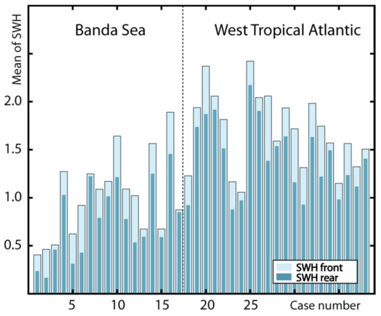
Figure 5.
Bar plots representing average significant wave heights (SWHs) for leading (i.e., front) and trailing (i.e., rear) sections (see text for details) of the ISWs for all cases in Table 1.
Table 2.
Mean of SWHs in front and rear of ISWs (see text for details) and differences between both (in percentage) for cases in the Banda Sea and Tropical West Atlantic. In light orange colors (bottom row), the same method is used for all Copernicus UFSAR cases (which are not exactly the same as those considered in gray shaded rows, see text for more details).
We therefore feel confident to propose as a possible interpretation for the observed decrease in SWH to the rear sections of an ISW as being the effects of ISWs in the local surface wave field, particularly the ISW-induced enhanced surface breaking. Since SWH is observed in the SAR altimeter to decrease as we move from unperturbed sections ahead of the ISW to sections behind the ISW (i.e., after the wave has passed), it is possible that a significant part of the surface wave spectrum is damped as a consequence of the passage of an ISW (in particular for the highest third of surface waves). This could be the result of assuming that additional surface wave breaking is triggered by the passing ISW, since this would cause the highest waves to increase beyond their limiting amplitude, break, and dissipate wave energy. In this case, the highest waves in the wave spectrum would undergo significant damping and cause a decrease in SWH in the transition between the ISWs’ rough and smooth sections—which we again recall is where whitecaps are consistently observed in optical imagery.
3.3. A Case Study Using Optical Imagery and Advanced SAR Altimeter Products
Figure 6 and Figure 7 concern the same data scene as in Figure 4 but regarding advanced SAR products, which are FFSAR and UFSAR with different retrackers, respectively (the retracker schemes are briefly described in Section 2.2.3). To calculate the SWH average cross-sections of ISWs, we used the average value within 10 km before and after the ISW center region (as conducted in Figure 4, which are about 4 km in length, but using the advanced SAR altimeter products described in Section 2.2.3). We coin the names “SWH-rear” and “SWH-front”, respectively.
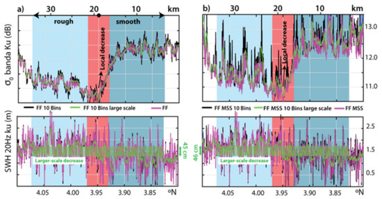
Figure 6.
The rectangles depicted in red shades represent the ISW center at 3.95°N. From the center of ISW, it is considered ±2 km to each side. To the left of it, we define the “SWH front” ahead of the ISW (“rough” in lighter blue using scales of about 10 km) and to the right, the “SWH rear” (“smooth” in darker blue using 10 km). Top of (a,b) shows along-track NRCSs (i.e., σ0) measured by the SRAL altimeter (in synergy with the OLCI) with the SAR-mode retracking color-coded in (a) FFSAR, FFSAR 10 Bins and its large-scale mean and in (b) FFSAR MSS, FFSAR MSS 10 Bins and its large-scale mean (using a box running average with approximately 3 km). Bottom plots show SWHs’ large-scale variations of 0.45 m in (a) and 0.46 m in (b), identified in the green shaded rectangles, when comparing the section in front of the primary ISW with that in the rear.
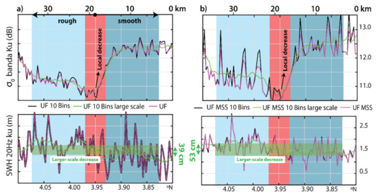
Figure 7.
As in Figure 6, but top of (a,b) shows along-track NRCSs (i.e., σ0) measured by the SRAL altimeter (in synergy with the OLCI) with the SAR-mode retracking color-coded in (a) UFSAR, UFSAR 10 Bins and its large-scale mean and in (b) UFSAR MSS, UFSAR MSS 10 Bins and its large-scale mean (using a box running average of 3 km). Bottom plots show SWHs’ large-scale variations of 0.39 m in (a) and 0.53 m in (b), identified in the green shaded rectangles, when comparing the section in front of the primary ISW with that in the rear for the same products.
The list used to evaluate the percentage difference between the front and rear of ISWs in these new algorithms is in Supplementary Materials S1 (see Table S1), being similar to Table 1. General remarks can be made regarding those advanced SAR processing results:
- Consistent results for all products: from Copernicus products, FF and UF full bins to FF and UF 10 bins processing schemes.
- SWHs from the Tropical Atlantic Ocean are higher than for the Banda Sea, which is understandable since in the Banda Sea, swell waves are practically absent; note that the average wave periods are 9.2 and 5.1 s, respectively.
- As expected, the adaptive MSS algorithms allow for better capturing of σ0 variations along the track, the 10 bin processing being a little more sensitive to heterogeneous sea surfaces.
- It is suggested however that the 10 bin processing has little impact on the SWH results for this applications and study regions.
- It is also suggested that the FFSAR processing (both schemes applied by CLS) has small impacts on SWH differences in this particular application (Internal Solitary Waves). It is as if by lowering the radar footprint, the processing is much less impacted by heterogeneities on the sea surface, making the MSS and 10 bin processing almost useless.
3.4. Results for Advanced FFSAR Products
More statistical analyses of the SWH variations between the front and rear of ISWs are presented in Figure 8, which are measured by the different unfocused and focused SAR processing configurations. Globally, the same results as those obtained in the case study of Section 3.3 are observed. In particular, it is confirmed that the adaptive MSS processing scheme tends to reduce the SWH attenuation in UFSAR, whereas it does not seem to impact the FF-SAR measurements, suggesting that the narrow footprint of the FFSAR makes the model less sensitive to the roughness inhomogeneities of the surface.
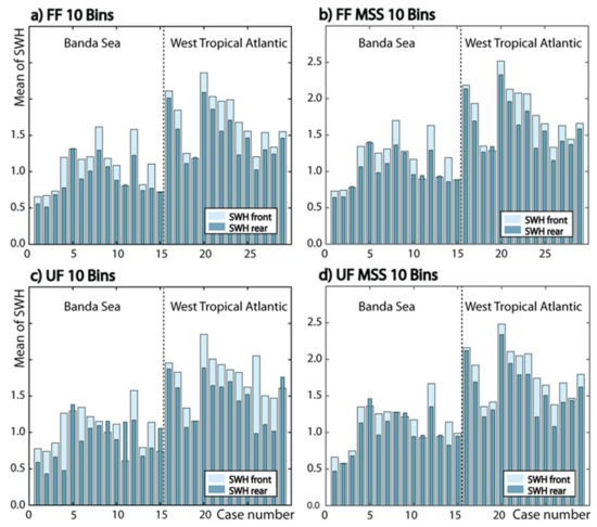
Figure 8.
Bar plots representing significant wave heights (SWHs) for leading (front) and trailing (rear) sections of the ISWs for all cases in Table S1 using different algorithms: (a) FF 10 Bins. (b) FF MSS 10 Bins. (c) UF 10 Bins. (d) UF MSS 10 Bins.
3.5. Consistency of Results for Different SAR Products
Table 2 demonstrates the consistency of results for all SAR products processed in this paper for SWHs. While the average attenuation in SWH is in the range 10–13% for the UFSAR 10 bin processing scheme that compares with 25% for the standard Copernicus products in the Banda Sea, for the West Tropical Atlantic off the Amazon river mouth, the range is between 11 and 17% in comparison with the 17% of the Copernicus products. Furthermore, in the FFSAR mode (and recalling that the processing is all using the 10 bin method), one can see that for the Banda Sea, the range is 12–16% in comparison with the 25% of the Copernicus standard processing, while for the Western Tropical Atlantic, the range in the FFSAR mode is 10–12% in comparison with the 17% in the standard UFSAR Copernicus processing scheme. We note that the adaptive MSS processing scheme (FF MSS 10 Bins and UF MSS 10 Bins in Table 2) gives systematically slightly smaller SWH attenuations than the SARmultilookLS3 ocean retracking algorithm (FF 10 Bins and UF 10 Bins in Table 2). All this said, the standing feature from Table 2 is the consistency of the average SWH attenuation for all products studied in this paper.
3.6. Image Processsing for the Investigation of Wave Breaking in Sentinel-2 Images
In this section, we calculate the percentage of whitecaps (or a fraction of wave breaking) in a specific MSI image of the Sentinel-2 satellite. The image was selected because there is synergy with the Sentinel-3B image shown in Figure 9a, which is from the Indian Ocean, in the Banda Sea, acquired on 21 April 2019. ISWs are clearly seen at −7.21°N and at −7.28°N in the Sentinel-2 and Sentinel 3B images, respectively, which were acquired with approximately a 3 h difference (see Figure 9a,b).
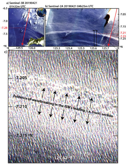
Figure 9.
(a) Quasi-true color image (Level-1b) acquired on 21 April 2019 at 01 h 31 m UTC by the OLCI sensor onboard the Sentinel-3B satellite. The red line represents the ground-track of the satellite, which in this case is practically parallel to the ISWs’ direction of propagation. (b) Image taken in the visible band by the Multispectral Instrument (MSI) onboard the Sentinel-2A satellite on 21 April 2019 at 04:25 UTC showing sea surface signatures of the same ISW packet seen in (a) approximately 3 h later. The red line also represents the ground-track of the satellite Sentinel-3 in the same day but at a different time. (c) Zoomed section of the leading ISW seen in (b). Note the bright spots aligned in bands, which are evidence of whitecaps generated by breaking surface waves.
We follow the methods published in Kubryakov et al. [42], which were applied for Landsat satellite data but can be adjusted to the MSI (see Section 2.4). Here we select an image section (corresponding to the black rectangle in Figure 9b), in the near-infrared NIR band (Band 8), that corresponds to the center wavelength of 842 nm in the Sentinel-2′ MSI and apply the methods described in Section 2.4.
Firstly, we verify the azimuthal angles that were found to be between 30° and 70°, in this specific case at around 35°. Band 10 is used to detect and discard high cirrus clouds, meaning that cirrus clouds are filtered with a threshold of 0.003. In this case, all pixels satisfy this criterion, and the image section is hence unaffected by high cirrus clouds. Then, we apply a wiener filter (see Figure 10), with a window size of 60 pixels (see Section 2.4 and [42]). This is a low-pass filter that is usually applied to an intensity image that has been degraded by constant power additive noise. The wave breaking fraction (W) is the difference between original Band 8 (NIR) and this filtered image (see Figure 10).
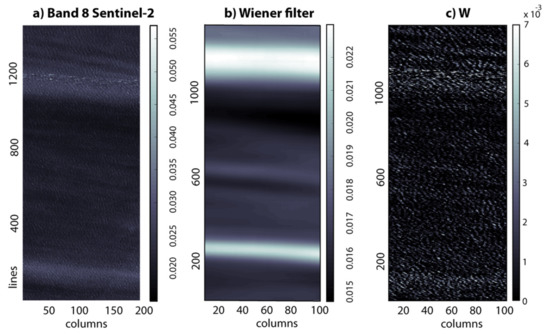
Figure 10.
(a) Zoom as shown in the black rectangle in Figure 9b corresponding to the NIR Band 8 of the Multispectral Instrument (MSI) onboard the Sentinel-2A satellite on 21 April 2019 at 04 h 25 m UTC showing sea surface signatures of an ISW packet. (b) Wiener filter applied to the image in part (a)—see text for details. (c) The image labeled W represents the wave breaking fraction, calculated by subtracting part (b) from (a).
As explained in Kubryakov et al. [42] and in Section 2.4, a suitable threshold to obtain the fraction of breaking is 0.002. The result is presented in Figure 11. Pixels where no breaking is detected are colored in white in Figure 11a, whereas the colored scale applies to the actual number of fractions of breaking. To comprehend the amount of breaking that is caused by the presence of the ISWs, we plot in Figure 11b an average profile along the ISW propagation direction. It can be seen that the fraction of wave breaking varies along the ISW direction, from 2.5 × 10⁻³ to more than 7.5 × 10⁻³. An average estimate of the fraction of breaking in a region unaffected by the ISW (ahead of the ISW packet) is 3.0 × 10⁻³ (not shown). This means that wave breaking is enhanced by at least two-fold over the sections of the ISW where surface wave breaking occurs. These results are important in the context of this work because they show by an independent method that wave breaking occurs for those ISWs typically analyzed in the altimeter records in the previous Sections. We note in passing that the wave breaking fractions found here are in line with similar values shown in Kubryakov et al. [42], who computed W values of the order of 7–10 × 10−3 for large ISWs near the Strait of Gibraltar (see their Figure 9b).
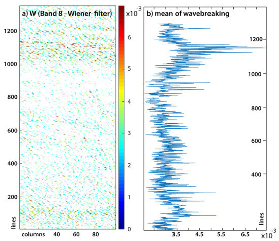
Figure 11.
(a) W represents wave breaking as shown in Figure 10c but color-coded to highlight the ISWs’ different sections, in which we applied a threshold of 0.002 (see text for details). (b) Mean of wave breaking fraction, i.e., W calculated for each line of (a), which is also approximately along the ISWs’ crests.
The same authors also estimate that the ISWs in their study enhance the fraction of breaking, i.e., whitecap enhancement, by a factor of 3 for a wind speed of about 10 m/s. In our study case of Figure 10 and Figure 11, the wind speed estimate is about 7 to 8 m/s, and the whitecap enhancement is at least two-fold and up to 7.5 × 10⁻³. Therefore, after the analysis explained in this Section, we are confident to say that significant wave breaking occurs for typical ISWs in the Banda Sea. The same procedure is more difficult to be applied to the Tropical West Atlantic, but we are confident that the wave breaking effect there is strong and similar to the Banda Sea.
We finally note that the case demonstrated in this Section, dated 21 April 2019, is of course a synergy case, presented in Table 1 (Section 3.2). The average SWH evaluated 10 km in front of the ISW located at 125.72°E, −7.28°N is 0.62 m, while the same average (in scales of 10 km) evaluated behind the ISW is of 0.31 m. In this case, the relative SWH decrease, presumably owing to breaking surface waves, is of 50%. We note however that, in such low wave height scenarios, the radar altimeter SWH measurements are probably less accurate and should be taken with caution.
4. Summary and Conclusions
This paper focuses on satellite remote sensing of Internal Solitary Waves (ISWs) by the new Synthetic Aperture Radar (SAR) altimeter on board Sentinel-3. We have pointed out that observations show that the sea surface roughness bands generated by ISWs often contain breaking waves having wavelengths of the order of meters and decameters (i.e., intermediate-scale waves, see Figure 1). Sometimes, such roughness bands containing breaking intermediate-scale waves have been observed when the sea surface was glassy with little or no surface winds. Investigations for oblique-looking satellite SAR imagers already show that non-polarized scattering mechanisms have to be invoked to explain radar backscattering from breaking waves adequately (see e.g., [25,47,48,49,50]) in the presence of inhomogeneous surface currents such as those produced near the surface by ISWs. These effects were hypothesized as the suppression of small-scale wind ripples by turbulence generated by breaking waves and were also recently confirmed by direct wave tank measurements described in Ermakov et al. [51].
While σ0 estimates relate more to small-scale roughness (elements with length scales greater than about three times the incident electromagnetic wavelength) rather than to some measure of the local wave spectrum (and hence with surface wave breaking), a more suited parameter to detect surface wave breaking could be SWH. As said before, this can be retrieved from satellite altimetry via the waveforms’ leading slopes. Note that SWH is, by design, a statistical parameter that conveys a measure of the significant wave height (traditionally the highest third of the surface wave field). Therefore, if the highest waves in the local (i.e., altimeter footprint) surface wave spectrum change—say by resonance with an ISW propagating below—then a measurable variation is expected to appear in the altimeter’s SWH estimates. More importantly, we expect a signal in SWH when these surface waves grow beyond their maximum equilibrium point and break causing wave energy dissipation behind the wave breaking band of the ISW surface manifestation.
Along-track SWH estimates from SAR altimeters revealed a sudden reduction in surface wave height owing to the presence of ISWs in the deep ocean. Recalling that energy in surface waves is proportional to the surface wave height squared, we propose an explanation for the decrease in wave energy after the passage of a large solitary wave: that the evidence of wave dissipation observed in the altimeter is due to breaking waves provoked by an internal wave—a surface wave interaction, presumably owing itself to resonance. The former argument is clearly consistent with the high resolution Multi-Spectral Instrument (MSI) Sentinel-2 shown in Figure 9, which reveals the existence of a region of enhanced meter-scale waves and whitecaps. We take this feature as evidence of strong wave breaking owing to a resonant interaction. This is a new and important result in oceanography, since ISWs may propagate at basin-scale distances (see e.g., [40]), meaning that they could cause a significant amount of enhanced surface turbulence along several hundred kilometers.
Furthermore, despite the altimeter evidence in this study concerning only large-scale ISWs, it has been shown that smaller-scale ISWs’ propagation over the shelf also feature enhanced surface breaking—this was shown e.g., using aerial LIDAR measurements of intermediate-scale ISWs (of the order a few hundreds of meters) in their dissipation stages off the west coast of Portugal [52]. Being a ubiquitous feature in both deep-ocean and coastal environments, ISWs may play a more efficient role than previously acknowledged in atmosphere-ocean interactions, owing to enhanced surface wave breaking. While energy input into the wave field by wind wave growth mechanisms may be enhanced by ISW resonant effects, it is eventually balanced by sinking terms owing to wave breaking, which generates turbulence and injects air bubbles into the upper water layer [52], typically across depth scales of the same order as the surface wave heights (as shown by Wang and Wijesekera [53]). We suggest that the breaking of surface waves owing to large amplitude ISWs may play a key role in the dynamics of the upper ocean, i.e., in the exchange of momentum, heat, and gases between the atmosphere and the ocean.
Energy in the surface wave field is slowly accumulated under the wind action over thousands of wave periods [11], being redistributed by nonlinear wave-wave interactions [54]. Interestingly, all that energy can be quickly cascaded down to turbulent scales and dissipation—owing to enhanced surface wave breaking from an ISW—within very short time scales (typically of the order of a single internal wave period, about 40 min). This is an important aspect about ISWs previously undocumented, provided there is a minimum amount of surface wave breaking, which can be caused when resonance occurs between ISWs and surface waves. When the ISW phase speed is large enough (e.g., in deep ocean regions), energy can be transferred between the ISW and surface waves with meter-scales, the latter being able to grow in amplitude and eventually break dissipating significant amounts of energy. Alternatively, or even simultaneously, it could also be possible that the presence of ISWs shifts the surface wave spectrum towards smaller wavelengths. A similar feature, but ascribed to other ocean phenomenon, was described in [55], who show a large attenuation in SWHs (measured by Jason-3) in the vicinity of the Gulf Stream off the coast of North America (see their Figure 3b). These authors noted large gradients in SWH in scales of 10 km as the altimeter footprints illuminate waves inside and outside the Gulf Stream by a factor of 2. Because of the current-wave interaction, it is likely that these large gradients in relatively short spatial scales may have to do with wave breaking and surface wave energy dissipation in a similar manner to the phenomena reported in this paper.
Satellite altimetry—including new-generation and more sophisticated missions (such as Sentinel-6 and the upcoming SWOT mission)—could prove a useful tool to understand and investigate these questions better. Note that, unlike imaging SARs, which have a limited number of acquisitions per orbit (owing to power limitations), satellite altimeters operate continuously and could (at least in principle) be used to map ocean internal waves on a routine and global basis and hence help quantify their turbulent dissipation more effectively.
Regarding the altimeter SAR processing, the consistency of the results between the different processing was demonstrated; both UFSAR and FFSAR (in full and reduced bins mode) are impacted by ISWs’ signatures in SWH and σ0. It does seem, however, more valuable and relevant to make use of higher sampling altimeter processing as the fully focused SAR may better detect small scale features (which would provide additionally a better gain in resolution as long as the vertical wave motion does not alter it that much). It must also be emphasized that further improvements would be made possible with the Sentinel-6 Open-burst operating mode (i.e., interleaved) which will not only reduce the noise of the altimeter measurements, but also significantly improve the focusing precision of the FFSAR measurements (an important step forward compared to the Cryosat-2 and Sentinel-3 missions which are currently impacted by sidelobes in the along-track point target response caused by the azimuth replicas of the Closed-burst mode).
Ultimately, surface wave breaking owing to ISWs add to the turbulent mixing and dissipation caused by breaking internal waves, both phenomena driving vertical transport of heat, carbon dioxide, and other climatologically important tracers in the ocean and at the air-sea interface. Consequently, ISWs play an important role in shaping the ocean circulation and distributions of heat and carbon within the climate system (see e.g., the review in [56]). The relative importance of surface wave breaking due to large ISWs in the deep ocean remains to be accounted for.
Supplementary Materials
The following supporting information can be downloaded at: https://www.mdpi.com/article/10.3390/rs14030587/s1, Table S1: List of Sentinel-3 cases in SAR-mode retracking approach exhibiting large-scale ISWs in optical imagery (OLCI) in synergy with the corresponding sea surface signatures in the SRAL altimeter. Note that cases are referring to the Banda Sea in the Indian Ocean before 27 September 2018, and the Tropical Western Atlantic after that, and that some dates include two or three ISWs, which were captured in the same image (i.e., relative orbit and cycle).
Author Contributions
Conceptualization, A.M.S.-F.; Data curation, A.M.S.-F. and S.A.; Formal analysis, A.M.S.-F.; Funding acquisition, J.C.B.d.S. and F.B. (Franck Borde); Investigation, A.M.S.-F., J.C.B.d.S., T.M. and C.M.; Methodology, A.M.S.-F., J.C.B.d.S. and T.M.; Project administration, F.B. (Franck Borde); Software, A.M.S.-F. and S.A.; Supervision, J.C.B.d.S.; Validation, F.B. (François Boy) and N.P.; Visualization, J.M.M.; Writing—original draft, A.M.S.-F. and J.M.M.; Writing—review and editing, J.C.B.d.S., T.M., C.M., F.B. (François Boy) and N.P. All authors have read and agreed to the published version of the manuscript.
Funding
This work has been funded by the European Commission (EC) and the European Space Agency (ESA). We thank “National Centre for Space Studies” (CNES) for technical support.
Data Availability Statement
The data presented in this study are openly available in Copernicus Open Access Hub: https://scihub.copernicus.eu/dhus/#/home, accessed on 27 December 2021.
Acknowledgments
This work was funded by the EU and ESA, under subcontract CLS-ENV-BC-20-0017 “Multi Sensor Synergy Study for Sentinel-3C/D” between the University of Porto and Collecte Localisation Satellites, SA. J.C.B.d.S. thanks the Portuguese funding agency Fundação para a Ciência e Tecnologia (FCT) under project UIDB/04683/2020. A.M.S.-F. gratefully acknowledges FCT and the UE for a Ph.D. grant SFRH/BD/143443/2019. J.M.M. thanks the FCT under projects UIDB/04423/2020 and UIDP/04423/2020. This paper is dedicated to Noddy, for his beloved companionship.
Conflicts of Interest
The authors declare no conflict of interest.
References
- Apel, J.R.; Byrne, H.M.; Proni, J.R.; Charnell, R.L. Observations of oceanic internal and surface waves from the earth resources technology satellite. J. Geophys. Res. Oceans 1975, 80, 865–881. [Google Scholar] [CrossRef]
- Fu, L.-L.; Holt, B. Seasat Views Oceans and Sea Ice with Synthetic-Aperture Radar; California Institute of Technology, Jet Propulsion Laboratory: Pasadena, CA, USA, 1982; Volume 81, p. 200. [Google Scholar]
- Apel, J.R.; Gonzalez, F.I. Nonlinear features of internal waves off Baja California as observed from the SEASAT imaging radar. J. Geophys. Res. Oceans 1983, 88, 4459–4466. [Google Scholar] [CrossRef]
- Alpers, W.; Salusti, E. Scylla and Charybdis observed from space. J. Geophys. Res. Oceans 1983, 88, 1800. [Google Scholar] [CrossRef]
- Kim, H.; Son, Y.B.; Jo, Y.-H. Hourly Observed Internal Waves by Geostationary Ocean Color Imagery in the East/Japan Sea. J. Atmos. Ocean. Technol. 2018, 35, 609–617. [Google Scholar] [CrossRef]
- Zhang, X.; Zhang, J.; Meng, J.; Fan, C.; Wang, J. Observation of internal waves with OLCI and SRAL on board Sentinel-3. Acta Oceanol. Sin. 2020, 39, 56–62. [Google Scholar] [CrossRef]
- Magalhaes, J.M.; Da Silva, J.C.B. Satellite Altimetry Observations of Large-Scale Internal Solitary Waves. IEEE Geosci. Remote Sens. Lett. 2017, 14, 1–5. [Google Scholar] [CrossRef]
- Santos-Ferreira, A.M.; Da Silva, J.C.B.; Magalhaes, J.M. SAR Mode Altimetry Observations of Internal Solitary Waves in the Tropical Ocean Part 1: Case Studies. Remote Sens. 2018, 10, 644. [Google Scholar] [CrossRef]
- Santos-Ferreira, A.M.; Da Silva, J.C.B.; Srokosz, M. SAR-Mode Altimetry Observations of Internal Solitary Waves in the Tropical Ocean Part 2: A Method of Detection. Remote Sens. 2019, 11, 1339. [Google Scholar] [CrossRef]
- Magalhães, J.; Alpers, W.; Santos-Ferreira, A.; da Silva, J. Surface Wave Breaking Caused by Internal Solitary Waves: Effects on Radar Backscattering Measured by SAR and Radar Altimeter. Oceanography 2021, 34, 166–176. [Google Scholar] [CrossRef]
- Babanin, A. Breaking and Dissipation of Ocean Surface Waves; Cambridge University Press: Cambridge, UK, 2011. [Google Scholar]
- Maury, M.F. The Physical Geography of the Sea and Its Meteorology; Harper: New York, NY, USA, 1861. [Google Scholar]
- Osborne, A.R.; Burch, T.L. Internal Solitons in the Andaman Sea. Science 1980, 208, 451–460. [Google Scholar] [CrossRef]
- Perry, R.B.; Schimke, G.R. Large-amplitude internal waves observed off the northwest coast of Sumatra. J. Geophys. Res. Oceans 1965, 70, 2319–2324. [Google Scholar] [CrossRef]
- New, A.; Da Silva, J. Remote-sensing evidence for the local generation of internal soliton packets in the central Bay of Biscay. Deep. Sea Res. Part I Oceanogr. Res. Pap. 2002, 49, 915–934. [Google Scholar] [CrossRef]
- Phillips, O.M. On the Interactions between Internal and Surface Waves. Izv. Atmos. Ocean. Phys. 1973, 9, 954–961. [Google Scholar]
- Lewis, J.E.; Lake, B.M.; Ko, D.R.S. On the interaction of internal waves and surface gravity waves. J. Fluid Mech. 1974, 63, 773–800. [Google Scholar] [CrossRef]
- Craig, W.; Guyenne, P.; Sulem, C. The surface signature of internal waves. J. Fluid Mech. 2012, 710, 277–303. [Google Scholar] [CrossRef]
- Kodaira, T.; Waseda, T.; Miyata, M.; Choi, W. Internal solitary waves in a two-fluid system with a free surface. J. Fluid Mech. 2016, 804, 201–223. [Google Scholar] [CrossRef]
- Taklo, T.M.A.; Choi, W. Group resonant interactions between surface and internal gravity waves in a two-layer system. J. Fluid Mech. 2020, 892, 14. [Google Scholar] [CrossRef]
- Lyzenga, D.R.; Bennett, J.R. Full-spectrum modeling of synthetic aperture radar internal wave signatures. J. Geophys. Res. Earth Surf. 1988, 93, 12345. [Google Scholar] [CrossRef]
- Plant, W.J.; Keller, W.C.; Hayes, K.; Chatham, G. Normalized radar cross section of the sea for backscatter: 1. Mean levels. J. Geophys. Res. Oceans 2010, 115, 09032. [Google Scholar] [CrossRef]
- Ochi, M.K.; Tsai, C.-H. Prediction of Occurrence of Breaking Waves in Deep Water. J. Phys. Oceanogr. 1983, 13, 2008–2019. [Google Scholar] [CrossRef][Green Version]
- Stokes, G.G. Supplement to a paper on the Theory of Oscillatory Waves. Math. Phys. Pap. 2010, 1, 314–326. [Google Scholar] [CrossRef]
- Kudryavtsev, V.; Kozlov, I.; Chapron, B.; Johannessen, J.A. Quad-polarization SAR features of ocean currents. J. Geophys. Res. Oceans 2014, 119, 6046–6065. [Google Scholar] [CrossRef]
- Brown, G. The average impulse response of a rough surface and its applications. IRE Trans. Antennas Propag. 1977, 25, 67–74. [Google Scholar] [CrossRef]
- Dinardo, S.; Lucas, B.; Benveniste, J. Sentinel-3 STM SAR ocean retracking algorithm and SAMOSA model. In Proceedings of the 2015 IEEE International Geoscience and Remote Sensing Symposium (IGARSS), Milan, Italy, 26–31 July 2015; pp. 5320–5323. [Google Scholar]
- Ray, R.D.; Mitchum, G.T. Surface manifestation of internal tides generated near Hawaii. Geophys. Lett. 1996, 23, 2101–2104. [Google Scholar] [CrossRef]
- Raney, R. The delay/Doppler radar altimeter. IEEE Trans. Geosci. Remote Sens. 1998, 36, 1578–1588. [Google Scholar] [CrossRef]
- Donlon, C.; Berruti, B.; Buongiorno, A.; Ferreira, M.-H.; Féménias, P.; Frerick, J.; Goryl, P.; Klein, U.; Laur, H.; Mavrocordatos, C.; et al. The Global Monitoring for Environment and Security (GMES) Sentinel-3 mission. Remote Sens. Environ. 2012, 120, 37–57. [Google Scholar] [CrossRef]
- Boy, F.; Desjonqueres, J.-D.; Picot, N.; Moreau, T.; Raynal, M. CryoSat-2 SAR-Mode Over Oceans: Processing Methods, Global Assessment, and Benefits. IEEE Trans. Geosci. Remote Sens. 2016, 55, 148–158. [Google Scholar] [CrossRef]
- Ray, C.; Martin-Puig, C.; Clarizia, M.P.; Ruffini, G.; Dinardo, S.; Gommenginger, C.; Benveniste, J. SAR Altimeter Backscattered Waveform Model. IEEE Trans. Geosci. Remote Sens. 2014, 53, 911–919. [Google Scholar] [CrossRef]
- Raynal, M.; Labroue, S.; Orsztynowicz, M.; Picot, N.; Guillot, A.; Boy, F. Sentinel-6A Delay Doppler Processing: Assessment over the Global Ocean. In Proceedings of the 2016 SAR Altimetry Workshop, La Rochelle, France, 31 October–1 November 2016. [Google Scholar]
- Egido, A.; Smith, W.H.F. Fully Focused SAR Altimetry: Theory and Applications. IEEE Trans. Geosci. Remote Sens. 2016, 55, 392–406. [Google Scholar] [CrossRef]
- Reale, F.; Carratelli, E.P.; Di Leo, A.; Dentale, F. Wave Orbital Velocity Effects on Radar Doppler Altimeter for Sea Monitoring. J. Mar. Sci. Eng. 2020, 8, 447. [Google Scholar] [CrossRef]
- Buchhaupt, C.; Fenoglio, L.; Becker, M.; Kusche, J. Impact of vertical water particle motions on focused SAR altimetry. Adv. Space Res. 2021, 68, 853–874. [Google Scholar] [CrossRef]
- Buchhaupt, C. Model Improvement for SAR Altimetry. Ph.D. Thesis, Schriftenreihe Fachriftenreihe Geodäsie der Technischen Universität Darmstadt, Darmstadt, Germany, 2019. [Google Scholar]
- Dinardo, S.; Fenoglio-Marc, L.; Becker, M.; Scharroo, R.; Fernandes, M.J.; Staneva, J.; Grayek, S.; Benveniste, J. A RIP-based SAR retracker and its application in North East Atlantic with Sentinel-3. Adv. Space Res. 2021, 68, 892–929. [Google Scholar] [CrossRef]
- Tourain, C.; Piras, F.; Ollivier, A.; Hauser, D.; Poisson, J.C.; Boy, F.; Thibaut, P.; Hermozo, L.; Tison, C. Benefits of the Adaptive Algorithm for Retracking Altimeter Nadir Echoes: Results From Simulations and CFOSAT/SWIM Observations. IEEE Trans. Geosci. Remote Sens. 2021, 59, 9927–9940. [Google Scholar] [CrossRef]
- Magalhaes, J.M.; da Silva, J.C.B.; Buijsman, M.C.; Garcia, C.A.E. Effect of the North Equatorial Counter Current on the generation and propagation of internal solitary waves off the Amazon shelf (SAR observations). Ocean Sci. 2016, 12, 243–255. [Google Scholar] [CrossRef]
- Jackson, C. Internal wave detection using the Moderate Resolution Imaging Spectroradiometer (MODIS). J. Geophys. Res. Oceans 2007, 112, 11. [Google Scholar] [CrossRef]
- Kubryakov, A.; Kudryavtsev, V.; Stanichny, S. Application of Landsat imagery for the investigation of wave breaking. Remote Sens. Environ. 2021, 253, 112144. [Google Scholar] [CrossRef]
- Lim, J.S. Two-Dimensional Signal and Image Processing; Prentice Hall: Englewood Cliffs, NJ, USA, 1990. [Google Scholar]
- Koepke, P. Effective reflectance of oceanic whitecaps. Appl. Opt. 1984, 23, 1816–1824. [Google Scholar] [CrossRef]
- Frouin, R.; Schwindling, M.; Deschamps, P.-Y. Spectral reflectance of sea foam in the visible and near-infrared: In Situ measurements and remote sensing implications. J. Geophys. Res. Earth Surf. 1996, 101, 14361–14371. [Google Scholar] [CrossRef]
- Liu, A.K.; Liu, C.-T.; Ming-Kuang, H.; Zheng, Q. Satellite Remote Sensing of South China Sea, 1st ed.; Liu, A.K., Ho, C.-R., Liu, C.-T., Eds.; Tingmao Publish Company: Taiwan, China, 2008; ISBN 978-986-122-948-5. [Google Scholar]
- Kudryavtsev, V.; Hauser, D.; Caudal, G.; Chapron, B. A semiempirical model of the normalized radar cross-section of the sea surface 1. Background model. J. Geophys. Res. Oceans 2003, 108, FET-2. [Google Scholar] [CrossRef]
- Kudryavtsev, V.; Akimov, D.; Johannessen, J.A.; Chapron, B. On radar imaging of current features: 1. Model and comparison with observations. J. Geophys. Res. Oceans 2005, 110, 07016. [Google Scholar] [CrossRef]
- Kudryavtsev, V.N.; Chapron, B.; Myasoedov, A.G.; Collard, F.; Johannessen, J.A. On Dual Co-Polarized SAR Measurements of the Ocean Surface. IEEE Geosci. Remote Sens. Lett. 2013, 10, 761–765. [Google Scholar] [CrossRef]
- Kudryavtsev, V.N.; Fan, S.; Zhang, B.; Mouche, A.A.; Chapron, B. On Quad-Polarized SAR Measurements of the Ocean Surface. IEEE Trans. Geosci. Remote Sens. 2019, 57, 8362–8370. [Google Scholar] [CrossRef]
- Ermakov, S.; Dobrokhotov, V.; Sergievskaya, I.; Kapustin, I. Suppression of Wind Ripples and Microwave Backscattering Due to Turbulence Generated by Breaking Surface Waves. Remote Sens. 2020, 12, 3618. [Google Scholar] [CrossRef]
- Magalhaes, J.M.; da Silva, J.C.B.; Batista, M.; Gostiaux, L.; Gerkema, T.; New, A.L.; Jeans, D.R.G. On the detectability of internal waves by an imaging lidar. Geophys. Res. Lett. 2013, 40, 3429–3434. [Google Scholar] [CrossRef]
- Wang, D.W.; Wijesekera, H.W. Observations of Breaking Waves and Energy Dissipation in Modulated Wave Groups. J. Phys. Oceanogr. 2018, 48, 2937–2948. [Google Scholar] [CrossRef]
- Lyzenga, D.R. Effects of nonlinear energy transfer on short surface waves. J. Geophys. Res. Oceans 2010, 115, 10001. [Google Scholar] [CrossRef]
- Ardhuin, F.; Gille, S.T.; Menemenlis, D.; Rocha, C.B.; Rascle, N.; Chapron, B.; Gula, J.; Molemaker, J. Small-scale open ocean currents have large effects on wind wave heights. J. Geophys. Res. Oceans 2017, 122, 4500–4517. [Google Scholar] [CrossRef]
- Whalen, C.B.; De Lavergne, C.; Garabato, A.C.N.; Klymak, J.M.; MacKinnon, J.A.; Sheen, K.L. Internal wave-driven mixing: Governing processes and consequences for climate. Nat. Rev. Earth Environ. 2020, 1, 606–621. [Google Scholar] [CrossRef]
Publisher’s Note: MDPI stays neutral with regard to jurisdictional claims in published maps and institutional affiliations. |
© 2022 by the authors. Licensee MDPI, Basel, Switzerland. This article is an open access article distributed under the terms and conditions of the Creative Commons Attribution (CC BY) license (https://creativecommons.org/licenses/by/4.0/).