Article

Practical Dynamical-Statistical Reconstruction of Ocean’s Interior from Satellite Observations

1
College of Meteorology and Oceanography, National University of Defense Technology, Hunan 410073, China
2
Beijing Institute of Applied Meteorology, Beijing 100029, China
*
Author to whom correspondence should be addressed.
Remote Sens. 2021, 13(24), 5085; https://doi.org/10.3390/rs13245085
Submission received: 3 August 2021 / Revised: 26 November 2021 / Accepted: 6 December 2021 / Published: 14 December 2021
(This article belongs to the Special Issue Remote Sensing of the Sea Surface and the Upper Ocean)

Abstract

:
The algorithms based on Surface Quasi-Geostrophic (SQG) dynamics have been developed and validated by many researchers through model products, however it is still doubtful whether these SQG-based algorithms are worth using in terms of observed data. This paper analyzes the factors impeding the practical application of SQG and makes amends by a simple “first-guess (FG) framework”. The proposed framework includes the correction of satellite salinity and the estimation of the FG background, making the SQG-based algorithms applicable in realistic circumstances. The dynamical-statistical method SQG-mEOF-R is thereafter applied to satellite data for the first time. The results are compared with two dynamical algorithms, SQG and isQG, and three empirical algorithms, multivariate linear regression (MLR), random forest (RF), and mEOF-R. The validation against Argo profiles showed that the SQG-mEOF-R presents a robust performance in mesoscale reconstruction and outperforms the other five algorithms in the upper layers. It is promising that the SQG-mEOF-R and the FG framework are applicable to operational reconstruction.

Graphical Abstract

1. Introduction

The satellite can provide a broad view on the ocean, while only the sea surface can be observed. Conversely, Argo profiles can reach as deep as 2000 m but are sparsely and loosely distributed. It is an important issue to project the satellite data into the interior of the ocean. This projection extends the conventional remote sensing and can thus be nominated as subsurface and deeper ocean remote sensing [1].
Pure empirical algorithms are typically employed in the subsurface reconstruction. One approach is to perform reconstruction by the superposition of empirical vertical modes, e.g., the Gravest Empirical Mode [2], Coupled Pattern Reconstruction [3], and mEOF-R (multivariate Empirical Orthogonal Function—Reconstruction) [4,5,6]. Although the empirical modes can represent multi-scale signals, the modes at one exact grid cannot actually be computed since Argo profiles are irregularly distributed. Only the approximate modes can be obtained, assuming that all of the profiles in the given temporal/spatial window share the same modes. The other approach is to perform surface-subsurface regression. This approach is favored, especially in recent years with the development of machine learning algorithms. The state-of-the-art machine learning algorithms can dig the nonlinear relation among the data at the expense of consuming more computational resources in the training phase. A good number of works have demonstrated the performance of the machine learning algorithms [7,8,9,10,11]. However, the nonlinear machine learning algorithms could possibly bring about negligible improvements or even take risks in deteriorating the performance of certain layers [7].
On the other hand, the algorithms based on Surface Quasi-Geostrophic (SQG) dynamics can retrieve subsurface density and geostrophic velocity from surface inputs and stratification profiles [12,13]. The SQG theory is a special case of quasi-geostrophic dynamics that is intended to highlight the role of surface buoyancy in mesoscale motions, such as frontogenesis [14,15]. The SQG solution is in substance a surface-trapped vertical mode that projects the surface buoyancy signal into the interior of the ocean [16]. However, the SQG mode is not enough to present robust performances since the interior of the ocean is driven by potential vorticity (PV). Isern-Fontanet et al. [17] proposed an eSQG (effective SQG) algorithm by estimating the PV of upper layers by surface buoyancy. Wang et al. [18] put forward the isQG (interior plus SQG) method by representing the interior solution with the barotropic mode and the first baroclinic mode. The isQG is still far from perfect due to the intrinsic surface-intensified shape of SQG mode and the first baroclinic mode [19]. Yan et al. [20] developed the SQG-mEOF-R algorithm by superimposing the dynamical mode of SQG and the empirical mode of EOF, which outperformed SQG and isQG, especially in the Peru–Chile upwelling domain. Nevertheless, almost all of these algorithms are applied to model products only.
To the best of our knowledge, only one study of practical application has ever been reported, which was the realistic application of isQG [21]. Unfortunately, the performances were quite poor in terms of satellite inputs. Liu et al. [21] attributed the poor performances to the erroneous remotely sensed Sea Surface Salinity (SSS) data. However, their utilization of monthly climatology as the background (so-called L17 Framework hereinafter) should also take responsibility. In the previous SQG works based on model products, a daily varying background, e.g., the low-pass-filtered background extracted from daily data, is typically employed. Compared to the non-static background, the monthly climatology makes the SQG solution less tenable and could thus lead to significant bias (see Section 2.4.1 for a detailed explanation).
In brief, an operational framework for the practical application of SQG-based algorithms is still lacking. In terms of observed data, no historical research has ever reported the comparison between pure empirical algorithms and those improved SQG algorithms, such as isQG and SQG-mEOF-R. It is especially questionable whether the SQG-based algorithms are worth using in this era of machine learning.
This paper proposes a first-guess (FG) scheme to operationally implement SQG-based algorithms and further validates the performance of SQG-mEOF-R by observational data. Two dynamical algorithms, SQG and isQG, and three empirical algorithms, including mEOF-R, multivariate linear regression (MLR), and random forest (RF), are used as baseline models.

2. Materials and Methods

2.1. Data Introduction

The sea surface temperature (SST) is extracted from the Reynolds OISST v2.1 dataset, which is a well-known product that fuses the temperature observations from satellite and in situ platforms by the Optimal Interpolation (OI) [22]. The Advanced Very-High-Resolution Radiometer (AVHRR)-only daily version was used in this paper. This is a product gridded on a 0.25° regular grid.
The Data Unification and Altimeter Combination System (DUACS) Absolute Dynamic Topography (ADT) product is a daily objective analysis product that combines the sea surface height (SSH) data from multi-platforms [23]. The delayed-time L4 reprocessed 0.25°/daily product (ID: SEALEVEL_GLO_PHY_CLIMATE_L4_REP_OBSERVATIONS_008_057) was obtained from Copernicus Marine Environment Monitoring Service (CMEMS). Besides the daily products, the monthly ADT climatology was calculated by the Mean Dynamic Topography (MDT) plus the monthly climatological Sea Level Anomaly (SLA) derived from the monthly SLA product of 2000–2018.
The ESA (European Space Agency)-CCI (Climate Change Initiative) SSS v1.8 is the latest version of satellite salinity products blending the remotely sensed salinity data of SMOS (Soil Moisture and Ocean Salinity) L2 ESA-OSv622/CATDS (Centre Aval de Traitement des Données SMOS) RE05, Aquarius L3 v5.0, and SMAP (Soil Moisture Active and Passive) L2 RSS (Remote Sensing Systems) v3.0 [24]. This product undergoes a series of calibrations and corrections and presents a high quality with the global root mean squared difference (RMSD) of 0.16 psu against Argo [25]. Note that the CCI SSS product is the only existing SSS product blending multi-platform satellite salinity observations. The daily running product was adopted. The nominal spatial resolution was 25 km. The SSS data were linearly gridded onto the regular grids of SST to compute the sea surface density (SSD).
The World Ocean Atlas (WOA) temperature/salinity monthly climatology is a gridded climatological mean dataset based on multi-source in situ observations [26]. The WOA13 monthly climatology used in this paper has the nominal spatial resolution of 0.25° and 57 uneven layers ranging from 0 to 1500 m.
The temperature/salinity (T/S) profiles of Global Observational Argo Dataset V3.0 were employed [27]. A series of “quality re-control” procedures were implemented to all of the real-time and delayed mode Argo profiles retrieved from the Global Data Assembly Center [28]. Only those adjusted data flagged as “good” were employed in this paper. Note that there are intensified 1-day profiles in 2014 provided by the project of Pacific Mode water Ventilation-Experiment (P-MoVE) [29].
The Global Reanalysis multi-model Ensemble Product (GREP) product is an ensemble product of four re-analyses, including GLORYS (Global ocean reanalysis) 2V4 [30], FOAM (Forecast Ocean Assimilation System) [31]-GLOSEA (Met Office Global Seasonal forecasting system) [32] 5v13, C-GLORS (CMCC-Global Ocean Reanalysis System) [33], and ORAS5 (Ocean Reanalysis System) [34,35]. Satellite SST, SSH, and multi-source in situ observations have been assimilated in the GREP dataset. The 0.25°/daily version utilized in this paper is available in CMEMS (ID: GLOBAL-REANALYSIS-PHY-001-031).

2.2. Data Preprocessing

The data of 2010–2013 and 2015–2017 are the training set, while the data of 2014 and 2018 are the validation set. The SSS, SST, ADT, ADT climatology, and WOA13 T/S climatology were interpolated onto the locations of Argo to obtain the collocated observation pairs. The shallowest T/S of Argo (must be <10 dbar) was taken as the near-surface temperature and salinity (NST/NSS). The Argo profiles and collocated climatological profiles were vertically interpolated onto 19 uneven layers of 10, 20, 30, 40, 50, 75, 100, 125, 150, 200, 250, 300, 400, 500, 600, 700, 800, 900, and 1000 dbar. Note that we chose 1000 dbar as the bottom since a good number of Argo profiles (about 12%) cannot reach 1000 dbar. The Steric Height (SH) and Dynamic Height (DH) were computed by S H z = 1 g H z 1 ρ 1 ρ 0 d z and D H z = 1 ρ 0 H z ρ d z , where H is the reference depth, i.e., 1000 dbar. The meaning of the other symbols can be found in Section 2.3.3. Since ADT is highly correlated to surface SH and surface DH (correlation coefficient > 0.9), an ADT-to-DH adjustment and an ADT-to-SH adjustment were carried out by the linear regression of longitude, latitude, and ADT with surface DH and surface SH to eliminate the height signal deeper than 1000 dbar.

2.3. Reconstruction Methods

2.3.1. MLR and RF

The regression of MLR (multivariate linear regression) and RF (random forest) was carried out between the surface layer and the 19 uneven layers. In the training phase, we used the collocated NST, NSS, ADT, longitude, and latitude as the predictors and the T or S at each layer as labeled data. The monthly climatology was firstly removed from the predictors and labeled data to build the surface–interior relation of anomalies. Each predictor was normalized by subtracting the mean value and then dividing the standard deviation. It must be noted that in some documents, the surface SH instead of ADT is used [11], however no significant differences can be seen between the results of surface SH and those of ADT since the surface SH has to be estimated by ADT. For RF or MLR, 2 (for T/S) × 19 (layers) regression models of monthly anomalies were trained. In the prediction phase, the gridded SST, SSS, ADT, and the longitude and latitude of the grid were input into 2 × 19 regression models to perform subsurface reconstruction. The reconstructed T/S were transformed into density to perform a further comparison with those SQG-based algorithms.
The random forest is an ensemble learning algorithm that randomly selects features and samples as the input of decision trees and then ensembles the results of the trees [36]. The most important parameters of RF are the number of trees (n_estimators) and the number of input features (or predictors) (n_features). Based on the scikit-learn toolkit of Python [37], we can directly use the GridSearchCV module to tune the parameters. The GridSearchCV performed an exhaustive search among all of the parameter combinations and chose the one that presents the best results of cross-validation (CV). We set the n_estimators as [50:50:300] and n_features as [1:1:5], and the best parameters were then automatically determined through a 10-fold CV.
Besides the subsurface reconstruction, RF also plays a role in SSS correction, which will be introduced in Section 2.4.3.

2.3.2. mEOF-R

The mEOF-R method is well-studied in previous works [4,5,6] and is thus not introduced in detail in this paper. In the training phase, mEOF-R extracts empirical modes (so-called mEOFs) based on the eigenvectors of the multivariate matrix X. The classical X is constructed by the profiles of T, S, and SH that are firstly interpolated onto the even layers of [10:10:1000] dbar. Since the magnitude of each variable is different, the profiles are normalized with regard to monthly climatology and standard deviation before they are input into the multivariate matrix. We computed different mEOFs at each grid of SST. Since no Argo is exactly located on the grids, a matchup of 10 degrees and 30 days was employed to make sure of the robustness of empirical modes. In the prediction phase, the depth-irrelevant amplitudes of at most three T/S/SH mEOFs can be estimated by the SST, SSS, and ADT-get SH (namely computed by the ADT-to-SH adjustment) so as to perform reconstructions. In this paper, three modes were employed to optimize the performance of the upper layers.

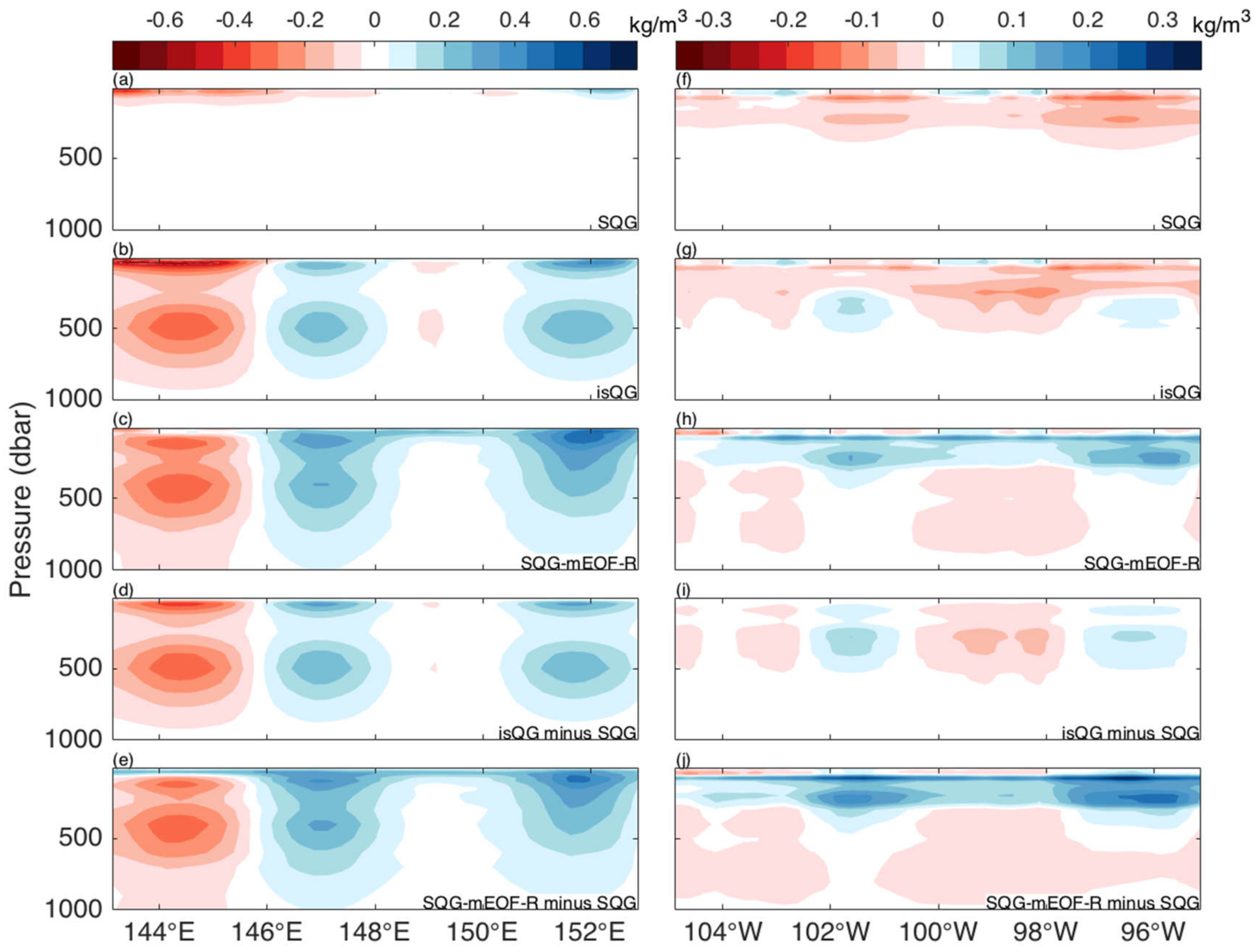
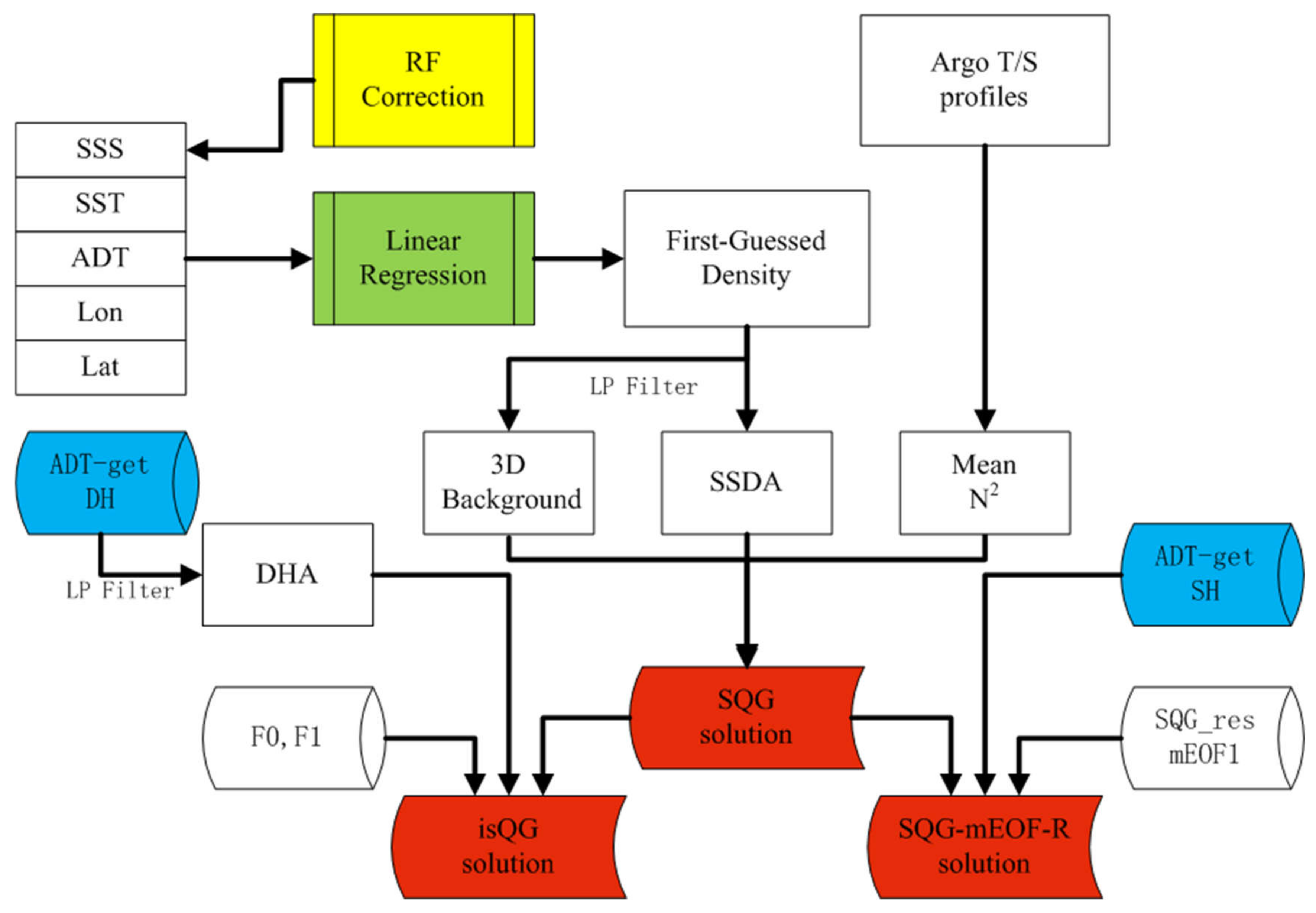
2.3.3. SQG, isQG, and SQG-mEOF-R

The Quasi-Geostrophic (QG) framework can be expressed as [38]:
L ψ + f 0 + β y = Q L = x 2 + y 2 + z f 0 2 N 2 z , H < z < 0
In Equation (1), ψ denotes the QG stream function, f0, β denotes the regional mean and meridional gradient of the Coriolis parameter, Q denotes the QG potential vorticity (QGPV), N2 denotes the buoyancy frequency, and H denotes the depth of the ocean bottom.
By a low-pass (LP) filter < >, the background should also satisfy Equation (1) in the form [18]:
L ψ + f 0 + β y = Q
After removing the background, the perturbation form that is used to perform reconstruction can be expressed as:
2 ψ + z f 0 2 N 2 ψ z = q ρ = ρ 0 f 0 g ψ z ;   V = z × ψ B . C .   ψ z | z = 0 = b | z = 0 f 0 = b s f 0 ;   ψ z | z = H = b | z = H f 0 = 0
Here, ψ and q are the perturbation forms of the QG stream function and QGPV, respectively, ρ denotes the density anomaly, V denotes the horizontal velocity anomaly, and bs =s0 is the surface buoyancy anomaly, calculated by the surface density anomaly, ρs, the volume mean density, ρ0, and the gravity acceleration, g.
Assuming that q = 0, the SQG equation is obtained. Based on sea surface density anomaly (SSDA) and regional mean, N2, the SQG solution can be computed in the Fourier space where the horizontal variation (namely the Laplace term) can be easily transformed into wavenumber [12].
The isQG assumes that the interior variation of QGPV can be decomposed into barotropic mode and baroclinic modes [18]. Based on the surface and bottom conditions of the stream function, the amplitudes of the barotropic mode (F0) and the baroclinic mode (F1) can be estimated by:
ψ ^ 0 = A 0 F 0 0 + A 1 F 1 0 + ψ ^ s 0 = g f 0 η ^ ψ ^ H = A 0 F 0 H + A 1 F 1 H + ψ ^ s H = 0
Here, ψ s denotes the SQG solution, A0 and A1 are the amplitudes, and η denotes the sea surface height (SSH) anomaly. The hat on the variables means the Fourier transformation. The reconstruction is then performed by ψ ^ = A 0 F 0 + A 1 F 1 + ψ ^ s .
Neither the SQG mode nor the first baroclinic mode, F1, could model subsurface-intensified eddies due to their surface-intensified shape [19]. Besides, it could possibly degrade the performance to use the uniform F1 derived from the regional mean, N2. The SQG-mEOF-R is proposed to replace the surface-intensified F1 with the empirical mode that differs at each grid [20]. The empirical mode is extracted following the same configurations and steps of mEOF-R, except for constructing the multivariate matrix by SQG-residual (SQG_res) density and SH profiles. The SQG_res profiles are computed by Argo profiles subtracting the collocated SQG solutions. Note that the SQG density should be theoretically projected by the surface “truth”, thus the SQG_res density mode should be zero at the surface. We processed the SQG_res density profiles by setting the surface value as zero and making the linear interpolation lie between the zero surface and thermocline (defined as the depth with the maximum N2 here). The SQG_res SH was also adjusted corresponding to the SQG_res density. Based on the empirical mode coupling SQG_res density and SH, the amplitude can be easily estimated by fitting the surface SH:
S H a = a 1 M 1 0
In Equation (5), SHa denotes the SQG-residual density, and a1 and M1 denote the amplitude and the first SH mode of mEOF. The density reconstruction (ρ) can be performed by the combination of the first density mode of mEOF (M1) and the SQG density ρSQG, namely: ρ = a 1 M 1 + ρ S Q G .

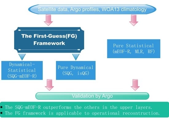
2.4. Proposal of the FG Framwrok

2.4.1. The L17 Framework

The implementation of SQG and isQG by Liu et al. [21] follows three main steps. Step 1: The sea surface height anomaly (SSHA) and sea surface density anomaly (SSDA) are calculated by ADT subtracting ADT monthly climatology, and satellite SSD subtracting monthly observational density climatology. Please note that “SSHA” instead of SLA is used since there is a matchup between the background of SSH and the background of density. Step 2: The SQG solution can be computed in the Fourier space by SSDA and the N2 profile through Equation (3), where the N2 profile is calculated from regional mean Argo T/S profiles. Then, the isQG solution can be solved by SSHA and the dynamical modes of F0 and F1 through Equation (4). Note that F0 and F1 are also computed from the regional mean, N2. Step 3: The complete solution can be obtained by the solution of step 2 plus the three-dimensional (3D) observational climatology.

2.4.2. Shortcomings of the L17 Framework

The L17 framework performed unsatisfactorily in the reconstruction based on observed data due to two dominant problems.
Problem 1: The satellite data, especially the SSS data, are erroneous or intrinsically different from the near-surface observations of Argo [39,40,41]. It is explicitly demonstrated in Equation (3) that the SQG solution is determined by the surface buoyancy, i.e., the surface density. As discussed in the L17 framework [21], the heavy bias of satellite SSS was the culprit of the failure of the reconstruction from satellite data. Nonetheless, a SSS correction module is not included in the L17 framework. In addition, the quality of the newest versions of SSS products has been significantly improved with the global RMSD of ~0.2 psu w.r.t Argo [42,43]. It implies that this problem can be solved by the employment of newly released SSS products and the import of a correction procedure.
Problem 2: The background field cannot be simply replaced by monthly climatology. Equation (3) can be taken for granted in the application to model products since the daily varying low-pass (LP)-filtered background can always be available. However, Equation (2) cannot be tenable in terms of the monthly climatology used in the L17 framework [21]. Consequently, Equation (3) would not be solved in the Fourier space unless the extra residuals of Equation (2) were compulsorily superimposed onto the perturbations. Systematic errors would be imposed when employing Equation (3) to perform reconstruction. The systematic errors do not only comprise of the biases between monthly climatology and daily varying background, but also include the biases of surface perturbation inherited from the climatology, which would be further projected into the interior of the ocean.

2.4.3. The FG Framework
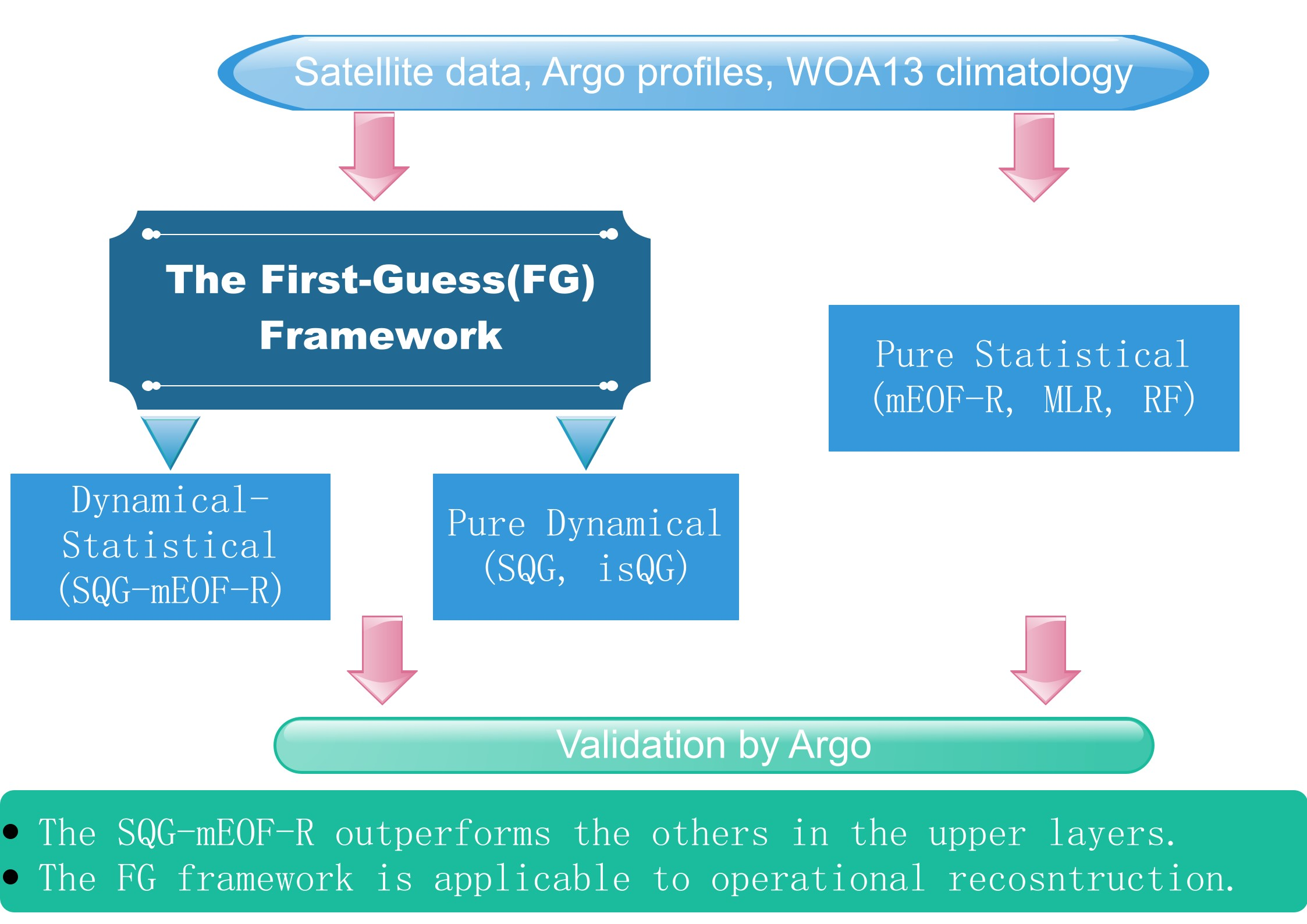
In order to solve these problems, the FG framework is proposed to make practical SQG-based reconstructions, as shown in Figure 1. Problem 1 can be improved by a SSS correction module based on the RF algorithm (the yellow part). The technique details are similar to the RF regression in Section 2.3.1, except for changing the predictors as longitude, latitude, SST, SSS, and ADT, and the labeled data as the Argo NSS. The corrected SSS along with the other satellite data would then be used to generate first-guessed fields based on the MLR regression. Problem 2 is circumvented by the estimation of a daily varying first-guessed background (the green part). The background is computed by carrying out a LP filter on the three-dimensional density reconstructed by MLR in Section 2.3.1. To be more specific, the quadratic surfaces are extracted from each layer of daily MLR reconstruction as the LP-filtered background [40]. The reason why we chose MLR instead of RF lies in the fact that the background estimated by two reconstructions would not differ significantly, while the MLR is more lightweight to become the pre-module of SQG reconstruction. Finally, we can compute the solution of SQG, isQG, and SQG-mEOF-R using the first-guessed background field, the sea surface density anomaly field, the regional mean N2 profile of Argo, and the adjusted surface DH or SH (the red part). The computation of the SQG solution and the isQG solution follows the same steps of the L17 framework, except for using the first-guessed background and the ADT-get DH. Please note that the surface DHA is also extracted by a LP filter in order to match the density background. The computation of SQG-mEOF-R is based on the SQG solution, the ADT-get SH, and the SQG-residual mEOF 1, as illuminated in Equation (5). Rather than performing 3D reconstruction directly, SQG-mEOF-R is implemented grid-by-grid.

3. Results

Two domains were selected to validate the reconstructions, including the North-West Pacific (NWP; 143° E–153° E, 25° N–35° N) and the South-East Pacific (SEP; 105° W–95° W, 15° S–25° S). The NWP is characterized by the Kuroshio current, where mesoscale eddies are ubiquitous, while the SEP is dominated by the Peru–Chile upwelling where there exist abundant subsurface-intensified eddies [44]. These two regions are aligned with the previous work of Yan et al. [20] so as to highlight the difference of model product application and practical application.
The RF correction has improved the quality of SSS. The root mean squared difference (RMSD) w.r.t Argo NSS was reduced from 0.14 to 0.13 psu in NWP and from 0.08 to 0.07 psu in SEP, while the correlation coefficient w.r.t Argo increased from 0.56 to 0.61 in NWP and from 0.90 to 0.93 in SEP. Note that the initial versions of SSS can be rather erroneous, e.g., the RMSD of monthly data can reach over 0.6 psu [45]. It indicates that the SSS CCI product has been a qualified one compared to initial versions of SSS products, thus the improvement of correction is limited. Nevertheless, the correction module is potentially useful considering the utilization of other SSS products in other regions, e.g., the RMSD of SMOS-only CATDS L3 products can be reduced from 0.367 to 0.255 psu in the Indian Ocean [46].
The bias of the surface density anomalies against WOA13 is 0.97 ± 0.45 kg/m3 in NWP and 0.13 ± 0.08 kg/m3 in SEP. Once the WOA13 were taken as the background, the heavy bias would be projected into the interior of the ocean. This systematic error could even exceed the error of surface density, since the salinity error of 0.2 psu usually corresponds to the density error of 0.1–0.2 kg/m3. The FG framework has effectively circumvented this problem, as the anomaly extracted from the low-pass filter is always zero-biased (namely, the mean value is close to zero). Note that the daily varying background estimated by the FG framework is based on the anomaly against WOA13, and thus the WOA climatology has been merged.
The reconstructed density fields of three SQG-based algorithms were compared through two zonal sections, as shown in Figure 2. The left panels show the section in NWP. This region is characterized by the strong but shallow pycnocline, which impedes the penetration of the SQG solution. As can be seen in Figure 2a, the SQG solution is trapped at upper 100 dbar and thus presents a negligible signal in the deeper ocean. The isQG solution and SQG-mEOF-R solution (Figure 2b,c) successfully project the surface signal into the ocean below the pycnocline. Consequently, the interior solution (isQG minus SQG) and the SQG-residual solution (SQG-mEOF-R minus SQG) present almost the same patterns with isQG and SQG-mEOF-R (Figure 2d,e). It turns out that the SQG solution loses its effectiveness in the NWP region, while the interior solution and SQG-residual solution dominate the interior signal of the ocean.
The right panels of Figure 2 show the section in SEP. In this region, the pycnocline is weak but deep, which is beneficial to the penetration of the SQG solution. In Figure 2f, the SQG solution can reach as deep as 300 dbar. The isQG solution (Figure 2g) is confined to upper 500 dbar and presents no more than two phases from surface to subsurface. The SQG-mEOF-R solution (Figure 2h) can present more complicated vertical structures, such as the warm-cold-warm three-compartment structure [44]. The pattern of SQG-mEOF-R is significantly different from that of the isQG solution or SQG solution. The SQG-residual solution presents a strong cold phase at 100–300 dbar and thus reverses the phase of the SQG solution (Figure 2j). In contrast, the interior solution of isQG (Figure 2i) only slightly adjusts the SQG solution, especially for upper 300 dbar. It implies that the SQG-mEOF-R has stronger potential to reconstruct complicated structures. Nevertheless, it is still doubtful whether the SQG-residual solution would bring about improvements instead of artifacts.
The RMSD and the spatial correlation of the reconstructions with regard to Argo are computed as the function of depth. The results of the test set are shown in Figure 3. As can be seen, the GREP product presents the best performance in both regions, which is not surprising since the Argo profiles have been assimilated in the product. In Figure 3a, all of the reconstructions present comparable RMSD except for the SQG and mEOF-R. The poor performance of mEOF-R indicates that the Argo profiles are still far from enough to extract robust empirical modes. Since the horizontal variation is quite strong in NWP, the profiles in the temporal and spatial window differ a lot from each other so that the mEOFs cannot represent the true variation of the given grid. The RMSD curves of isQG, SQG-mEOF-R, RF, and MLR are similar. The largest RMSD locates at about 50 dbar, corresponding to the shallow but strong mixed layer base. At 200–400 dbar, the RF and isQG are slightly better than SQG-mEOF-R, succeeded by the MLR.
In Figure 3b, the lowest correlation locates at 200–250 dbar, which is much deeper than the maximum RMSD layer. The SQG solution is extremely poor with the correlation lower than 0.5 at 200–700 dbar, partly due to the strong and shallow pycnocline. The correlation coefficient of mEOF-R strays away from other algorithms at deeper than 400 dbar, indicating that interior variation below pycnocline is still too strong to be caught by the empirical modes. As a result, the correlation of SQG-mEOF-R is also degraded. Conversely, the performances of RF and MLR at >400 dbar are much better. Nonetheless, the SQG-mEOF-R outperforms RF and MLR at upper 250 dbar, which highlights the advantage of the dynamical-statistical design of SQG-mEOF-R.
In the previous works about model product application, the isQG was believed to be intrinsically applicable to the strong currents [18,47] and presented comparable performances to SQG-mEOF-R [20]. However, at upper layers above 300 dbar in Figure 3b, the correlation of isQG is unexpectedly low. Combined with low RMSD of isQG in Figure 3a, it turns out that the baroclinic mode computed by regional mean stratification can successfully estimate the amplitude of the density field, but fails to retrieve the horizontal structures.
The performances of SQG-mEOF-R are prominent in Figure 3c,d, with a significant reduction of RMSD at 100–300 dbar and a significant improvement of correlation at 100–200 dbar. Satisfactory reconstructions can also be seen in terms of isQG or even the simple SQG. As concluded in [20], the weak pycnocline facilitates the penetration of SQG mode, making SQG-based algorithms more applicable in SEP than in NWP. In addition, since the horizontal variation is also weak in SEP, the extracted empirical modes or the first baroclinic mode are more robust. As a result, the mEOF-R also presents acceptable performances in SEP. On the other hand, the RF and MLR suffer from over-fitting, with a relatively low RMSD but a poor correlation at 100–150 dbar. It turns out that the regression relation drawn by the machine learning algorithm of RF is inferior to the simplest SQG mode at upper layers in SEP.
Abnormal peaks are reconstructed by SQG, isQG, and mEOF-R in Figure 3b. The unsatisfactory performances of these three coincide with the low correlation revealed by Figure 3b. The series of SQG and isQG present discrepancies with regard to Argo, and a significant reversed phase can be seen after day 200. Consequently, correlation coefficients of SQG and isQG are −0.56 and −0.12, respectively. It turns out that neither SQG nor the isQG solution are applicable at the upper layers of NWP. The series of MLR (yellow) is generally aligned with Argo, with a relatively low RMSD of 0.07 kg/m3 and high correlation of 0.62. Note that the SQG-based reconstructions are computed by the first guess of MLR. Hence, the unsatisfactory performances of SQG and isQG indicate that SQG mode and the first baroclinic mode are problematic or at least not representative. The SQG-mEOF-R, however, has successfully reproduced the general tendency of Argo series, with the RMSD of 0.05 kg/m3 and the correlation of 0.75. It turns out that the SQG mode plus the empirical mode is beneficial for the reconstruction, while the first baroclinic mode cannot model the true pattern of the upper layers.
Taking the high-frequency Argo profile (float number: 2,901,565) as an example, the performance of mesoscale reconstruction is highlighted in Figure 4. In Figure 4a, we can see that the float is caught by a series of energetic mesoscale eddies. The Argo is at first carried by an anti-cyclonic eddy and the trajectory gradually becomes cyclonic from day 150, and then becomes anti-cyclonic again from day 220. In Figure 4b, the corresponding low–high–low-density variation can be witnessed, and the corners of the trajectory in Figure 4a have their counterparts in the local peaks of the time series (the red line) in Figure 4b.
On the other hand, the machine learning algorithm of RF cannot outperform the MLR despite the increase in computational cost. The time series of RF (purple) even presents the opposite phase to Argo. Consequently, the correlation of RF is close to zero. It suggests that the machine learning algorithm takes risks in deteriorating the performance.
Figure 5 depicts the pattern of density anomalies of Argo 2,901,565 and the patterns of reconstructions. It can be seen that the basic patterns are successfully retrieved by 5 algorithms, except for the significant overestimation of mEOF-R in eddy centers. The warm center at approximately 300–600 dbar and day 110–125 (Figure 5a) is reconstructed by mEOF-R (Figure 5b), isQG (Figure 5e), and SQG-mEOF-R (Figure 5f), but fails to be estimated by MLR (Figure 5c) and RF (Figure 5d). In addition, the zero anomalies at 200 dbar and day 160–200 are only retrieved by MLR and SQG-mEOF-R, corresponding to the results in Figure 4. Although the performances of isQG and RF at 200 dbar are inferior to MLR in Figure 4, the correlation of the former two at all depths is still superior to the latter one in Figure 5. It indicates that the isQG and RF present merits in estimating the structures that are less energetic. The pattern of SQG-mEOF-R is closest to that of Argo, with the lowest RMSD and best correlation among all 5 algorithms. Nevertheless, none of the 5 reconstructions could present a robust performance at upper 50 dbar. The reconstruction of mixed layers is still a difficult task for the existing techniques.
Taking the GREP product as the reference, horizontal patterns can also be compared. It must be noted that it is tricky to take the mesoscale motions in GREP as the truth. Although the statistics in Figure 3 are supportive of the high quality of GREP, the Argo profiles used in validation are in substance not independent of GREP reanalysis. As depicted in Figure 6a, the GREP mainly presents four eddies, i.e., eddy 1 (143° E–146° E, 24° N–27° N), eddy 2 (149° E–152° E, 24° N–26° N), eddy 3 (148° E–151° E, 30° N–32° N), and eddy 4 (147° E–149° E, 26° N–29° N). These four eddies were successfully reconstructed by the algorithms in this paper, except SQG. Overestimation of eddies 1 and 4 can be seen in mEOF-R, MLR, RF, and SQG-mEOF-R. Meanwhile, eddy 4 of GREP presents a one-core pattern, however a two-core pattern can be seen in Figure 6c–g. Generally speaking, the performance in reconstructing mesoscale structures is comparable for mEOF-R, MLR, RF, and SQG-mEOF-R, however the mEOF-R tends to produce non-physical artifacts.
The horizontal pattern in Figure 6h is much simpler. The most conspicuous structure is the warm phase extending from left to right. The SQG reconstruction and isQG reconstruction present a quite uniform warm center in the middle of Figure 6i,l. The mEOF-R reconstruction still presents non-physical artifacts by estimating too many small eddies (Figure 6j). The MLR, RF, and SQG-mEOF-R successfully retrieve the extension-like pattern, however the former two misplace the center and significantly overestimate the warm phase. In the SEP region, the horizontal pattern is more difficult to reconstruct via existing methods. The SQG-mEOF-R turned out to be the most applicable algorithm.
In order to make further comparison against GREP, we compute the STD of different reconstructions with regard to GREP, as shown in Figure 7. In the NWP region, the SQG and mEOF-R present significantly high STD against GREP. The MLR and RF present a high STD center at (145° E–146° E, 32° N), which does not appear on isQG and SQG-mEOF-R reconstructions. The SQG-mEOF-R also presents several high STD centers, which partly coincide with the centers of mEOF-R. It indicates that the problem of mEOF-R is more or less inherited by SQG-mEOF-R. In terms of the SEP region, three SQG-based reconstructions present a low level of STD against GREP. The mEOF-R reconstruction is poorly aligned with GREP and presents several high STD centers. The STD pattern of MLR is similar to that of RF and shows a significantly high STD center at the southwest of the region. The results imply that the RF reconstruction can be more consistent with GREP than isQG and SQG-mEOF-R in NWP, however the superiority of SQG-based algorithms stands out in SEP.

4. Discussion

The technique of the pure empirical algorithm is favored by researchers in recent years, due to the rapid development of machine learning algorithms. The overall performance of RF is superior to MLR, as shown in Figure 3 and Figure 5. Nevertheless, the time series in Figure 4 demonstrates that the machine learning algorithm could possibly deteriorate the performance. Note that the typical circumstance is the low RMSD along with the poor correlation. Although RF is an ensemble learning algorithm that is claimed to lower the risk of over-fitting, the well-tuned RF is still powerless to retrieve the structures at upper layers.
The dynamical algorithms of SQG and isQG performed poorly in NWP (upper panels in Figure 3). The better performance of MLR has eliminated the possibility of the erroneous background. Thus, the main problem lies in the SQG and the first baroclinic mode (F1). The poor performance of SQG was not surprising as the SQG mode was trapped by the shallow and strong pycnocline (see Figure 2). However, it is disappointing that isQG cannot even outperform the linear regression in NWP, since isQG is meant to be applicable in the strong currents [18,47]. The degradation of isQG in realistic application is likely owing to the utilization of a regional mean F1. The significant horizontal variation in the Kuroshio current decreases the representativeness of F1. This problem is not noticeable in the application to model simulation but stands out in the realistic circumstance, where neither the surface nor the background is accurate. As a result, the error statistics (RMSD and STD) of isQG are satisfactory in Figure 3, Figure 6 and Figure 7, however the correlation is quite poor in Figure 3b. In the SEP, the weak stratification and better horizontal homogeneity facilitate the SQG and isQG (lower panels in Figure 3). Even the simplest SQG is more representative than the surface-subsurface relation derived from random forest (Figure 3d). The SQG-mEOF-R is comparable to RF at upper layers of NWP and outperforms RF at almost all depths of SEP. It turned out that the dynamical-statistical method can be more applicable than the complicated random forest algorithm.
The results are also supportive of the robustness of the FG framework. Compared to the L17 framework, the FG framework eliminates the bias of the input surface anomaly and provides a robust daily varying background. The FG framework thus makes Equations (2) and (3) tenable and prevents the projection of the bias of ~0.97 kg/m3 (in NWP) or ~0.13 kg/m3 (in SEP) into the interior of the ocean. The sea surface salinity is also a source of reconstruction error, while the utilization of CCI SSS effectively lowered the uncertainty of surface density. Although, the surface RMSD can never become zero in Figure 3 due to the intrinsic difference between satellite observation and in situ observation, e.g., the sub-footprint variation [39,41].
The SQG-mEOF-R is still facing problems in terms of practical application. The biggest headache lies in the extraction of empirical modes in the inhomogeneous regions, such as the Kuroshio current, where the number of Argo profiles is far from enough to extract a representative mode. The mEOFs must be computed by the profiles in a wide temporal and spatial window, while the profiles can be significantly different from each other. Consequently, the mEOFs can generally retrieve the mean state but cannot represent the variations. Evidence can be seen in the significantly low correlation of mEOF-R in those less energetic layers deeper than 400 dbar in Figure 3b. Similarly, the degradation of SQG-mEOF-R is also noticeable in Figure 3b. A better way to exploit the limited Argo profiles turned out to be the geography-based regression, namely taking longitude and latitude as factors. Future works are considered in terms of the combination of SQG and geography-based machine learning.
The validation of the mesoscale structure is still not perfectly solved by the existing data. Although the reanalysis data can be taken as the reference, it is still unknown whether the mesoscale eddies in the reanalysis are true. Note that the validation of reanalysis is also based on sparse Argo profiles, not to mention that these Argo profiles have been assimilated in the reanalysis.

5. Conclusions

This paper proposed an FG scheme to carry out SQG-based algorithms in the practical application, based on which the dynamical-statistical algorithm SQG-mEOF-R was validated by observed data for the first time. The results showed the robustness of the FG scheme, which contributed to the better performances of SQG, isQG, and SQG-mEOF-R in the weak-stratified and relatively homogeneous SEP region.
The vertical modes were not representative enough in the inhomogeneous NWP region due to the lack of Argo profiles. It is a disappointing conclusion that isQG was not quite applicable in the practical reconstruction in strong currents. Meanwhile, the poor empirical mode also degraded the performance of SQG-mEOF-R. Nonetheless, the SQG-mEOF-R presented better performance at upper layers and performed satisfactory work in retrieving the mesoscale variations of the 1-day Argo profile.
The machine learning algorithm random forest can perform well in subsurface reconstruction, especially considering the incorporation of longitude and latitude as factors. Nevertheless, the improvement from linear regression to machine learning can be negligible. There are circumstances in which the random forest algorithm is even inferior to linear regression due to the over-fitting problem.
The results in this paper highlighted that SQG-mEOF-R can be more powerful than the “shallow” machine learning algorithm of random forest at upper layers, especially in the South-East Pacific region. Besides pursuing deep machine learning algorithms, the technique of the dynamical-statistical method is worth investigating in the future.

Author Contributions

Conceptualization, H.Y. and R.Z.; methodology, H.Y.; software, C.B.; validation, H.Y., S.B. and H.W.; formal analysis, H.Y.; investigation, H.Y.; resources, H.Y.; data curation, H.W.; writing—original draft preparation, H.Y.; writing—review and editing, H.W., S.B. and H.Y.; visualization, H.Y.; supervision, R.Z. and C.B.; project administration, R.Z.; funding acquisition, R.Z. and H.W. All authors have read and agreed to the published version of the manuscript.

Funding

This paper is funded by the National Natural Science Foundation of China (41976188) and the National Key R&D Program of China (2018YFC1406202).

Data Availability Statement

The Global Argo Observational Dataset is distributed by China Argo Real-Time Data Center: Argo Real-time data-China Argo Real-time Data CenterThe OISST data are available at: https://climatedataguide.ucar.edu/climate-data/sst-data-noaa-high-resolution-025x025-blended-analysis-daily-sst-and-ice-oisstv2. The SSS CCI product can be available at: https://climate.esa.int/en/odp/#/project/sea-surface-salinity. The WOA13 monthly climatology can be downloaded from: https://climatedataguide.ucar.edu/climate-data/world-ocean-atlas-2013-woa13. The DUACS daily and monthly sea surface height data (ID: SEALEVEL_GLO_PHY_CLIMATE_L4_REP_OBSERVATIONS_008_057) and the reanalysis dataset of GREP (ID: GLOBAL-REANALYSIS-PHY-001-031) can be available from CMEMS: https://resources.marine.copernicus.eu/. The MDT is available from the Archiving, Validation, and Interpretation of Satellite Oceanographic Data (AVISO) website: https://www.aviso.altimetry.fr/es/data/products/. All of the links are last accessed on 13 December 2021.

Acknowledgments

We appreciate the three reviewers for their valuable suggestions.

Conflicts of Interest

The authors declare no conflict of interest.

References

  1. Klemas, V.; Yan, X.-H. Subsurface and Deeper Ocean Remote Sensing from Satellites: An Overview and New Result. Prog. Oceanogr. 2014, 122, 1–9. [Google Scholar] [CrossRef]
  2. Mitchell, D.A.; Wimbush, M.; Watts, D.R.; Teague, W.J. The residual GEM technique and its application to the southwestern Japan/East Sea. J. Atmos. Ocean. Technol. 2004, 21, 1895–1909. [Google Scholar] [CrossRef] [Green Version]
  3. Buongiorno, B.B.; Santoleri, R. Reconstructing synthetic profiles from surface data. J. Atmos. Ocean. Technol. 2004, 21, 694–703. [Google Scholar] [CrossRef]
  4. Buongiorno Nardelli, B.; Santoleri, R. Methods for the reconstruction of vertical profiles from surface data: Multivariate analyses, residual GEM, and variable temporal signals in the North Pacific Ocean. J. Atmos. Ocean. Technol. 2005, 22, 1762–1781. [Google Scholar] [CrossRef]
  5. Buongiorno Nardelli, B.; Cavalieri, O.; Rio, M.H.; Santoleri, R. Subsurface geostrophic velocities inference from altimeter data: Application to the Sicily Channel (Mediterranean Sea). J. Geophys. Res. Oceans 2006, 111, 1–22. [Google Scholar] [CrossRef]
  6. Buongiorno Nardelli, B.; Guinehut, S.; Verbrugge, N.; Cotroneo, Y.; Zambianchi, E.; Iudicone, D. Southern Ocean mixed layer seasonal and interannual variations from combined satellite and in situ data. J. Geophys. Res. Oceans 2017, 122, 10042–10060. [Google Scholar] [CrossRef] [Green Version]
  7. Bao, S.; Zhang, R.; Wang, H.; Yan, H.; Yu, Y.; Chen, J. Salinity profile estimation in the Pacific Ocean from satellite surface salinity observations. J. Atmos. Ocean. Technol. 2019, 36, 53–68. [Google Scholar] [CrossRef]
  8. Su, H.; Wu, X.; Yan, X.H.; Kidwell, A. Estimation of subsurface temperature anomaly in the Indian Ocean during recent global surface warming hiatus from satellite measurements: A support vector machine approach. Remote Sens. Environ. 2015, 160, 63–71. [Google Scholar] [CrossRef]
  9. Su, H.; Li, W.; Yan, X.H. Retrieving Temperature Anomaly in the Global Subsurface and Deeper Ocean From Satellite Observations. J. Geophys. Res. Oceans 2018, 123, 399–410. [Google Scholar] [CrossRef]
  10. Su, H.; Yang, X.; Lu, W.; Yan, X.H. Estimating subsurface thermohaline structure of the global ocean using surface remote sensing observations. Remote Sens. 2019, 11, 1598. [Google Scholar] [CrossRef] [Green Version]
  11. Buongiorno Nardelli, B. A Deep Learning Network to Retrieve Ocean Hydrographic Profiles from Combined Satellite and In Situ Measurements. Remote Sens. 2020, 12, 3151. [Google Scholar] [CrossRef]
  12. LaCasce, J.H.; Mahadevan, A. Estimating subsurface horizontal and vertical velocities from sea-surface temperature. J. Mar. Res. 2006, 64, 695–721. [Google Scholar] [CrossRef] [Green Version]
  13. Klein, P.; Hua, B.L.; Lapeyre, G.; Capet, X.; Le Gentil, S.; Sasaki, H. Upper ocean turbulence from high-resolution 3D simulations. J. Phys. Oceanogr. 2008, 38, 1748–1763. [Google Scholar] [CrossRef] [Green Version]
  14. Lapeyre, G.; Klein, P. Dynamics of the upper oceanic layers in terms of surface quasigeostrophy theory. J. Phys. Oceanogr. 2006, 36, 165–176. [Google Scholar] [CrossRef]
  15. Lapeyre, G. Surface Quasi-Geostrophy. Fluids 2017, 2, 7. [Google Scholar] [CrossRef]
  16. Lapeyre, G. What Vertical Mode Does the Altimeter Reflect? On the Decomposition in Baroclinic Modes and on a Surface-Trapped Mode. J. Phys. Oceanogr. 2009, 39, 2857–2874. [Google Scholar] [CrossRef]
  17. Isern-Fontanet, J.; Lapeyre, G.; Klein, P.; Chapron, B.; Hecht, M.W. Three-dimensional reconstruction of oceanic mesoscale currents from surface information. J. Geophys. Res. Oceans 2008, 113, 1–17. [Google Scholar] [CrossRef] [Green Version]
  18. Wang, J.; Flierl, G.R.; Lacasce, J.H.; Mcclean, J.L.; Mahadevan, A. Reconstructing the ocean’s interior from surface data. J. Phys. Oceanogr. 2013, 43, 1611–1626. [Google Scholar] [CrossRef]
  19. Assassi, C.; Morel, Y.; Vandermeirsch, F.; Chaigneau, A.; Pegliasco, C.; Morrow, R.; Colas, F.; Fleury, S.; Carton, X.; Klein, P.; et al. An Index to Distinguish Surface- and Subsurface-Intensified Vortices from Surface Observations. J. Phys. Oceanogr. 2016, 46, 2529–2552. [Google Scholar] [CrossRef]
  20. Yan, H.; Wang, H.; Zhang, R.; Chen, J.; Bao, S.; Wang, G. A Dynamical-Statistical Approach to Retrieve the Ocean Interior Structure From Surface Data: SQG-mEOF-R. J. Geophys. Res. Oceans 2020, 125, 1–15. [Google Scholar] [CrossRef]
  21. Liu, L.; Peng, S.; Huang, R.X. Reconstruction of ocean’s interior from observed sea surface information. J. Geophys. Res. Oceans 2017, 122, 1042–1056. [Google Scholar] [CrossRef]
  22. Reynolds, R.W.; Smith, T.M.; Liu, C.; Chelton, D.B.; Casey, K.S.; Schlax, M.G. Daily high-resolution-blended analyses for sea surface temperature. J. Clim. 2007, 20, 5473–5496. [Google Scholar] [CrossRef]
  23. Ducet, N.; Le Traon, P.Y.; Reverdin, G. Global high-resolution mapping of ocean circulation from TOPEX/Poseidon and ERS-1 and -2. J. Geophys. Res. Oceans 2000, 105, 19477–19498. [Google Scholar] [CrossRef]
  24. Boutin, J.; Vergely, J.-L.; Koehler, J.; Rouffi, F.; Reul, N. ESA Sea Surface Salinity Climate Change Initiative (Sea_Surface_Salinity_cci): Version 1.8 data collection. Available online: https://catalogue.ceda.ac.uk/uuid/9ef0ebf847564c2eabe62cac4899ec41 (accessed on 5 December 2021).
  25. Martin, A.; Guimbard, S.; Boutin, J.; Reul, N.; Catany, R. Overview of the CCI+SSS Project. Available online: https://meetingorganizer.copernicus.org/EGU2020/EGU2020-11683.html (accessed on 5 December 2021).
  26. Locarnini, R.A.; Levitus, S.; Boyer, T.; Antonov, J.I.; Mishonov, A.V.; Garcia, H.E.; Zweng, M.; Reagan, J.R. World Ocean Atlas 2013: Improved vertical and horizontal resolution. In Proceedings of the AGU Fall Meeting, San Francisco, CA, USA, 3–7 December 2012. [Google Scholar]
  27. Li, Z.Q.; Liu, Z.H.; Lu, S.L. Global Argo data fast receiving and post-quality-control system. In Proceedings of the IOP Conference Series: Earth and Environmental Science, Beijing, China, 18–20 November 2020; Volume 502. [Google Scholar]
  28. Argo Argo Float Data and Metadata from Global Data Assembly Centre (Argo GDAC). Available online: https://www.seanoe.org/data/00311/42182 (accessed on 5 December 2021).
  29. Xie, S.P. Advancing climate dynamics toward reliable regional climate projections. J. Ocean Univ. China 2013, 12, 191–200. [Google Scholar] [CrossRef] [Green Version]
  30. Lellouche, J.M.; Le Galloudec, O.; Drévillon, M.; Régnier, C.; Greiner, E.; Garric, G.; Ferry, N.; Desportes, C.; Testut, C.E.; Bricaud, C.; et al. Evaluation of global monitoring and forecasting systems at Mercator Océan. Ocean Sci. 2013, 9, 57–81. [Google Scholar] [CrossRef] [Green Version]
  31. Blockley, E.W.; Martin, M.J.; McLaren, A.J.; Ryan, A.G.; Waters, J.; Lea, D.J.; Mirouze, I.; Peterson, K.A.; Sellar, A.; Storkey, D. Recent development of the Met Office operational ocean forecasting system: An overview and assessment of the new Global FOAM forecasts. Geosci. Model Dev. 2014, 7, 2613–2638. [Google Scholar] [CrossRef] [Green Version]
  32. Maclachlan, C.; Arribas, A.; Peterson, K.A.; Maidens, A.; Fereday, D.; Scaife, A.A.; Gordon, M.; Vellinga, M.; Williams, A.; Comer, R.E.; et al. Global Seasonal forecast system version 5 (GloSea5): A high-resolution seasonal forecast system. Q. J. R. Meteorol. Soc. 2015, 141, 1072–1084. [Google Scholar] [CrossRef]
  33. Storto, A.; Masina, S.; Navarra, A. Evaluation of the CMCC eddy-permitting global ocean physical reanalysis system (C-GLORS, 1982-2012) and its assimilation components. Q. J. R. Meteorol. Soc. 2016, 142, 738–758. [Google Scholar] [CrossRef]
  34. Zuo, H.; Balmaseda, M.A.; Mogensen, K. The new eddy-permitting ORAP5 ocean reanalysis: Description, evaluation and uncertainties in climate signals. Clim. Dyn. 2017, 49, 791–811. [Google Scholar] [CrossRef]
  35. Zuo, H.; Balmaseda, M.A.; Tietsche, S.; Mogensen, K.; Mayer, M. The ECMWF operational ensemble reanalysis-analysis system for ocean and sea ice: A description of the system and assessment. Ocean Sci. 2019, 15, 779–808. [Google Scholar] [CrossRef] [Green Version]
  36. Huang, B.F.F.; Boutros, P.C. The parameter sensitivity of random forests. BMC Bioinformatics 2016, 17, 331. [Google Scholar] [CrossRef] [PubMed] [Green Version]
  37. Pedregosa, F.; Varoquaux, G.; Gramfort, A.; Michel, V.; Thirion, B.; Grisel, O.; Blondel, M.; Prettenhofer, P.; Weiss, R.; Dubourg, V.; et al. Scikit-learn: Machine learning in Python. J. Mach. Learn. Res. 2011, 12, 2825–2830. [Google Scholar] [CrossRef]
  38. Pedlosky, J. Geophysical fluid dynamics.; Springer: New York, NY, USA, 1979; ISBN 3540903682. [Google Scholar]
  39. Boutin, J.; Chao, Y.; Asher, W.E.; Delcroix, T.; Drucker, R.; Drushka, K.; Kolodziejczyk, N.; Lee, T.; Reul, N.; Reverdin, G.; et al. Satellite and In Situ Salinity: Understanding Near-Surface Stratification and Subfootprint Variability. Bull. Am. Meteorol. Soc. 2016, 97, 1391–1407. [Google Scholar] [CrossRef] [Green Version]
  40. Bao, S.; Wang, H.; Zhang, R.; Yan, H.; Chen, J. Comparison of Satellite-Derived Sea Surface Salinity Products from SMOS, Aquarius, and SMAP. J. Geophys. Res. Oceans 2019, 124, 1932–1944. [Google Scholar] [CrossRef]
  41. Yan, H.; Wang, H.; Zhang, R.; Bao, S.; Chen, J.; Wang, G. The Inconsistent Pairs Between In Situ Observations of Near Surface Salinity and Multiple Remotely Sensed Salinity Data. Earth Sp. Sci. 2021, 8, 1–15. [Google Scholar] [CrossRef]
  42. Vinogradova, N.; Lee, T.; Boutin, J.; Drushka, K.; Fournier, S.; Sabia, R.; Stammer, D.; Bayler, E.; Reul, N.; Gordon, A.; et al. Satellite salinity observing system: Recent discoveries and the way forward. Front. Mar. Sci. 2019, 6, 1–23. [Google Scholar] [CrossRef]
  43. Reul, N.; Grodsky, S.A.; Arias, M.; Boutin, J.; Catany, R.; Chapron, B.; D’Amico, F.; Dinnat, E.; Donlon, C.; Fore, A.; et al. Sea surface salinity estimates from spaceborne L-band radiometers: An overview of the first decade of observation (2010–2019). Remote Sens. Environ. 2020, 242, 111769. [Google Scholar] [CrossRef]
  44. Zhang, Z.; Zhang, Y.; Wang, W. Three-compartment structure of subsurface-intensified mesoscale eddies in the ocean. J. Geophys. Res. Oceans 2017, 122, 1653–1664. [Google Scholar] [CrossRef]
  45. Boutin, J.; Martin, N.; Yin, X.; Font, J.; Reul, N.; Spurgeon, P. First assessment of SMOS data over open ocean: Part II-sea surface salinity. IEEE Trans. Geosci. Remote Sens. 2012, 50, 1662–1675. [Google Scholar] [CrossRef] [Green Version]
  46. Bao, S.; Zhang, R.; Wang, H.; Yan, H.; Chen, J.; Wang, Y. Correction of Satellite Sea Surface Salinity Products Using Ensemble Learning Method. IEEE Access 2021, 1, 99. [Google Scholar] [CrossRef]
  47. Liu, L.; Peng, S.; Wang, J.; Huang, R.X. Retrieving density and velocity fields of the ocean’s interior from surface data. J. Geophys. Res. Oceans 2014, 119, 8512–8529. [Google Scholar] [CrossRef] [Green Version]
Figure 1. Technique flow of the FG scheme.
Remotesensing 13 05085 g001
Figure 2. Comparison of the sections of SQG-based solutions. The left panels (ae) present the 26.125° N section of NWP on 19 July 2014, while the right panels (fj) present the 20.125° S section of SEP on 4 April 2018. From top to bottom: SQG solution (a,f), isQG solution (b,g), SQG-mEOF-R solution (c,h), isQG minus SQG (d,i), and SQG-mEOF-R minus SQG (e,j). Note that the solutions are in the perturbation form without adding on the background.
Remotesensing 13 05085 g002
Figure 3. RMSD and correlation coefficient of the density reconstructions w.r.t Argo as the function of depth. From left to right: RMSD (a,c) and correlation coefficient (b,d). From top to bottom: NWP (a,b) and SEP (c,d). The dotted lines show the statistics of the GREP dataset.
Remotesensing 13 05085 g003
Figure 4. (a) Trajectory of the Argo 2901565. The Argo moved from light-dark points to deep-dark points, with the labeled number denoting the day of the year in 2014. (b) Time series of Argo density and the reconstructed density at 200 dbar. The statistics in the bracket show the RMSD and the correlation coefficient (Corr) of the reconstruction against Argo 2,901,565. The x-axis is the day of the year in 2014.
Remotesensing 13 05085 g004
Figure 5. Time-depth plot of the density anomalies of Argo 2,901,565 (a) and the reconstructions of mEOF-R (b), MLR (c), RF (d), isQG (e), and SQG-mEOF-R (f). The anomalies are calculated by subtracting the monthly climatology of WOA13. The statistics above (bf) show the RMSD and correlation of the pattern of each panel against the pattern of Argo in (a). X-axis is the day of the year in 2014.
Remotesensing 13 05085 g005
Figure 6. Comparison of the horizontal slices. The left panels (ag) present the 200 dbar slice of NWP on 19 July 2014, while the right panels (hn) present the 150 dbar slice of SEP on 4 April 2018. From top to bottom: GREP (a,h), SQG reconstruction (b,i), mEOF-R reconstruction (c,j), MLR reconstruction (d,k), isQG reconstruction (e,l), RF reconstruction (f,m), and SQG-mEOF-R reconstruction (f,n).
Remotesensing 13 05085 g006
Figure 7. The standard derivation of reconstructions with regard to GREP. The left panels (af) present the STD at 200 dbar in NWP, while the right panels (gl) present the STD at 150 dbar in SEP. From top to bottom: SQG reconstruction (a,g), mEOF-R reconstruction (b,h), MLR reconstruction (c,i), isQG reconstruction (d,j), RF reconstruction (e,k), and SQG-mEOF-R reconstruction (f,l).
Remotesensing 13 05085 g007
Publisher’s Note: MDPI stays neutral with regard to jurisdictional claims in published maps and institutional affiliations.

