Cramér-Rao Bound of Joint DOA-Range Estimation for Coprime Frequency Diverse Arrays

Abstract

Frequency diverse array (FDA) produces a beampattern with controllable direction and range by slightly shifting the carrier frequencies across the elements, which is attractive in many applications. By further incorporating coprime array structure and coprime frequency offsets, improved degrees-of-freedom and spatial/range resolutions have been achieved. For such a relatively new array configuration, theoretical performance analyses are essential to explore the potentials and to facilitate practical implementation. In this work, we consider coprime-FDA-based joint/separate angle-range estimation of far-field targets that exhibit two different types of Swerling fluctuation behavior, which are respectively modelled as deterministic and stochastic sources. Analytical expressions of the Cramér–Rao bounds (CRB) and numerical simulations for both cases are provided. The results reveal that the relationship between CRB and coprime FDA parameters is not simply monotonic. As shown in the numerical simulations, the CRB of coprime FDA outperforms that of uniform FDA-MIMO for more than $60\%$ under commonly-adopted coprime patterns. The presented results can be used as a guideline for optimal design of coprime FDA.

1. Introduction

The concept of frequency diverse array (FDA) was first proposed by Antonik et al. in 2006 [1,2]. In the pioneer work, a small and progressive frequency offset upon the carrier frequency is applied across the radiating elements. The use of element-to-element frequency offset generates a time-range-angle-dependent beampattern. Such a pattern is highly attractive for numerous applications including radar target localization [3,4,5], synthetic aperture radar (SAR) imaging [6,7], and wireless communications [8], since it enhances the flexibility of beam scanning and offers the potential to resist interference in a specific spatial region [9]. Nevertheless, the FDA beampattern generally exhibits periodicity in angle, range, and time [10,11]. Additionally, a standard FDA, i.e., a uniform linear FDA employing linearly increasing frequency offsets, yields coupling angle and range responses in the far-field beampattern. These unfavorable characteristics conspire to a spatiotemporal periodic S-shaped energy distribution in the angle-range plane, which further leads to ambiguity in target localization.

Owing to the fact that the FDA beampattern distribution can be controlled by tuning the frequency offsets, various solutions, such as time-dependent [12], logarithmic [13,14], and random [15] offsets, have been suggested to achieve a spatial-focusing and also preferably a time-invariant beampattern. Some sophisticated selection mechanisms have also been designed, which includes a transmit subarray strategy [16], adaptive selection scheme [17], and a multi-carrier transmission scheme [18,19], to name but a few. Additionally, by imposing certain evaluation metrics and penalty functions, the problem of frequency offset selection can be recast as an optimization problem [19]; different algorithms [20,21,22] have been employed to determine the optimal frequency offset.

The FDA angle-range estimation can also be decoupled from an array structure perspective. For example, many efforts have been made to incorporate the multiple-input multiple-output (MIMO) concept into FDA [4,23,24] to form a range-dependent-only beampattern. For MIMO enjoys the merits of increased degrees-of-freedom (DoF) and spatial diversity gain [25], it has attracted considerable interests. On the other hand, several types of sparse arrays have emerged to provide an enlarged array aperture and to overcome the DoF limitation for a given number of physical sensors. Among these sparse arrays, nested and co-prime configurations are compelling because they are more flexible and permit systematical design guided by explicit close-form expression [26,27]. But the latter is usually preferred, primarily due to the reduced mutual coupling [28,29]. FDA-MIMO radars exploit the DoF in the angle-range domain to jointly estimate the direction and range parameters of the targets [23]. In order to further achieve an improved DoF and spatial/range resolutions, a coprime FDA is proposed [30]. On the one hand, by incorporating the idea of coprime sampling to circumvent the limitation of physical sampling and using the virtual difference coarray concept, coprime FDA shows prominent advantages in terms of DOA-range resolution, localization accuracy, and the number of resolvable targets. Under the space-frequency difference equivalence of a coprime FDA, the unqiue non-negative lags of coarray produce extensive DoFs compared to the physical array [31]. On the other hand, the robustness of the coprime configuration in spatially filtering the interference [32] shows huge potential of adaptive beamforming using coprime FDA.

Objective performance analysis and optimal subarray design strategy are of paramount importance for arrays in practice, and they are often interconnected. In general, the Cramér–Rao bound (CRB) serves as a statistical benchmark to evaluate the degree of suboptimality that a certain unbiased parameter estimator exhibits. CRB also provides insights into the optimization of the array structure (cf., e.g., [20,33,34,35]). In the field of array signal processing, conventional research with respect to CRB mostly focuses on DOA estimation [36,37,38]. Motivated by the potentials of coprime FDAs and given the fact that their CRBs with respect to joint DOA-range estimation and the dependence between joint and separate estimations remain as yet uninvestigated, the technical contributions of this work are threefold, which are summarized as follows.

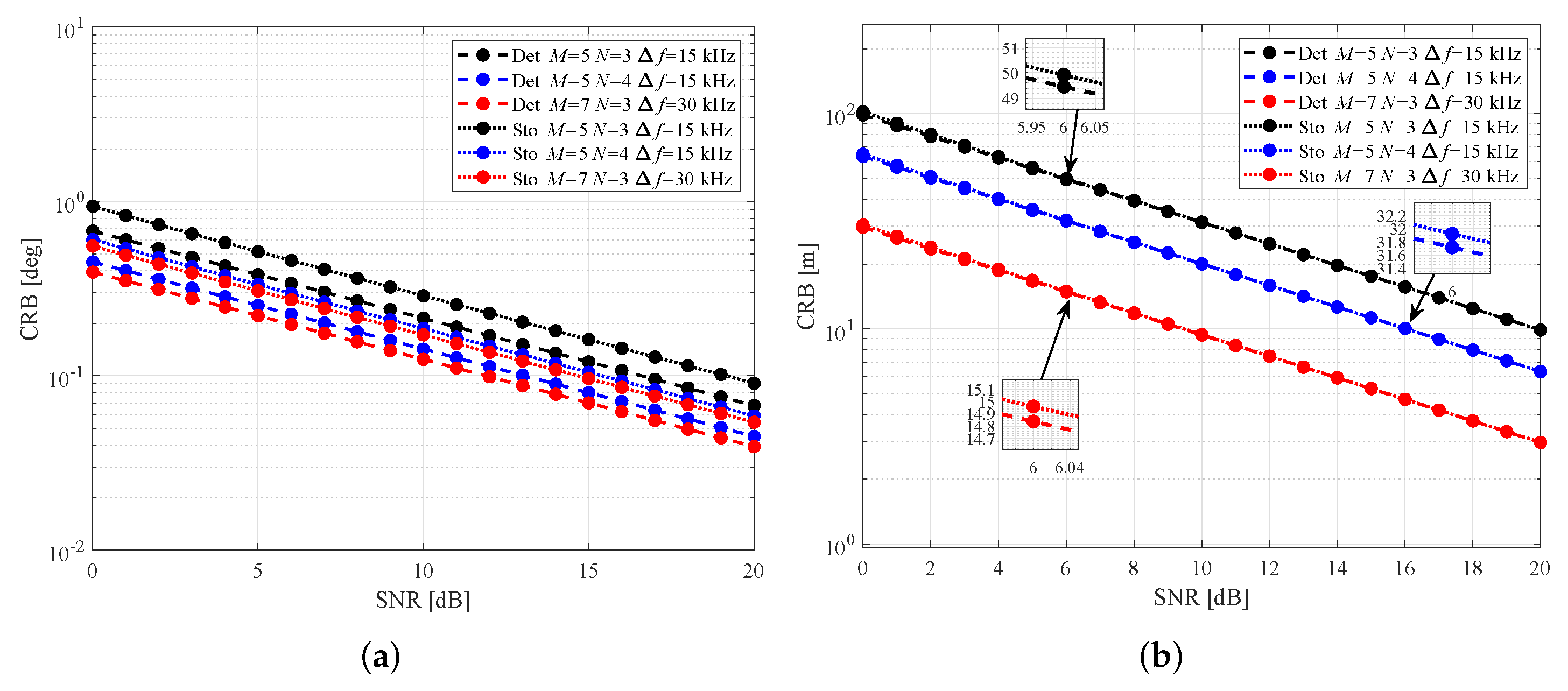
• In an attempt to capture the amplitude fluctuation of a target signal return due to the temporal variations of radar cross-section (RCS), Swerling models were established. Swerling 0 model [39,40] is associated with non-fluctuating RCS, and the radar return of such a target type shows deterministic characteristics. For complex targets that have many small surfaces and joints with different orientations, a Swerling I target-type model [41] is used, and the corresponding receive signal is subject to a stochastic model. In this work, we investigate far-field target detection, and both deterministic and stochastic signal models are considered.
• CRB identifies the potential performance of a signal model with the variance lower bound of unbiased estimation. For DOA-range estimation, the prior information of the radar target makes an impact on the CRB result. In this work, this issue is described as separate parameter estimation, i.e., CRB of DOA (range) estimation while range (DOA) is known. The relation between CRB of separate parameter estimation and CRB of joint estimation is studied via Fisher information with respect to angle and range.
• Analytical form expressions are derived for the input signal-to-noise ratio (SNR) and CRBs of DOA and range. Accordingly, numerical simulations are presented to compare CRBs for deterministic and stochastic source cases, and separate parameter estimation and joint estimation models. According to the analyses of CRB results, an intuitive method for coprime FDA design is proposed based on CRB minimization.

This paper is organized as follows. In Section 2, the configuration of coprime FDA and the transmit-receive steering vectors in deterministic case and stochastic cases are formulated. Based on the steering vectors, the array signal model is given. In Section 3, the explicit analytical form CRBs of joint estimation and separate estimation in deterministic signal cases are derived in terms of Gaussian distribution probability density function (PDF). When it comes to the stochastic signal case, the CRB is derived on the basis of the matrix form solution [42] in Section 4. Moreover, Section 5 presents some numerical simulations of CRBs in deterministic and stochastic source cases for different uniform FDA structures and coprime FDA structures. The comparisons of CRBs in different scenarios, i.e., two kinds of statistical characteristics and joint/separate estimation are analyzed. Ultimately, we make our conclusion in Section 6.

Notations: Lower (upper)-case bold characters are used to denote vectors (matrices). Vectors are by default in column orientation. ${(·)}^{\mathrm{T}}$ and ${(·)}^{\mathrm{H}}$ respectively represent the transpose and Hermitian operators of a matrix. $\mathrm{tr}\left(·\right)$ returns the trace of a matrix. Symbol ⊙ stands for the Hardmard-product. $\mathbb{E}\left[·\right]$ returns the expected value of a discrete random variable. ∇ is the Nabla symbol. ℜ returns the real part of a complex value. Operators ${(·)}^{\perp }$ represents the ortho-complement of a projector matrix.

2. Signal Model

In this work we consider a coprime FDA that consists of two collocated uniform linear subarrays. The transmit and receive subarrays respectively have N and M elements, where N and M are coprime integers. The array configuration of the coprime FDA is illustrated in Figure 1.

We assume that the unit inter-element spacing d is $\lambda /2$, where $\lambda$ denotes the wavelength. For a coprime FDA, a frequency increment as a multiple of $\Delta f$ is applied across the array element. As such, the carrier frequency of the nth transmit element can be expressed as

$$f_n=f_0+(n-1)·M·\Delta f,n=1,2,\cdots ,N,$$

(1)

where $f_0$ represents the FDA carrier frequency.

In array signal processing, the modelling of signal sources commonly falls into two categories [43], i.e., the deterministic and stochastic models. The former model category is adopted to describe the Swerling 0 type radar targets [39,40] and also in wireless communications [44]. The latter is related to Swerling I type targets and generic interferences [45] in radar applications as well as acoustic signals [46], where the signals are assumed to be driven by a Gaussian random process. In the following, we investigate radar detection performance for Swerling 0 and I targets, where the receive signals are respectively represented by deterministic and stochastic models.

2.1. Deterministic Signal Model

We first establish a deterministic signal model in this subsection. As stated above, we assume that a $priori$ knowledge on the scattered waveform from the target is accessible to the radar operators. Consider a far-field Swerling 0 target at position ($\theta ,r$), where $r\in [0,\mathrm{c}/2\Delta f]$ denotes the range from the far-field target to the first element and $\theta \in [-\pi /2,\pi /2]$ denotes the angle between arrival direction and array normal. Then, in the transmit stage, the phase of the signal radiated from the first element is

$$\begin{array}{c}\hfill {\phi }_1=\frac{2\pi f_1}{\mathrm{c}}r.\end{array}$$

(2)

Likewise, we can express the phase of the signal transmitted from the second element as

$$\begin{array}{c}\hfill {\phi }_2=\frac{2\pi f_2}{\mathrm{c}}(r-Mdsin\theta )=\frac{2\pi (f_0+M\Delta f)}{\mathrm{c}}(r-Mdsin\theta ).\end{array}$$

(3)

The phase difference between the first and the second elements caused by the path length difference is

$$\begin{array}{c}\hfill \Delta {\phi }_2={\phi }_2-{\phi }_1=\frac{2\pi }{\mathrm{c}}(-f_{0}Md·sin\theta +M\Delta f·r-M^2\Delta fd·sin\theta ).\end{array}$$

(4)

Similarly, the phase of the signal transmitted from the nth transmit element is

$$\begin{array}{c}\hfill {\phi }_n=\frac{2\pi f_n}{\mathrm{c}}(r-(n-1)Mdsin\theta )=\frac{2\pi (f_0+M(n-1)\Delta f)}{\mathrm{c}}(r-(n-1)Mdsin\theta ).\end{array}$$

(5)

The phase difference $\Delta {\phi }_n$ between the first and the nth transmit element is

$$\begin{array}{c}\hfill \Delta {\phi }_n={\phi }_n-{\phi }_1=\frac{2\pi }{\mathrm{c}}\left[-f_0(n-1)Md·sin\theta +(n-1)M\Delta f·r-M^2{(n-1)}^2\Delta fd·sin\theta \right].\end{array}$$

(6)

By taking the first transmit element as the reference, the transmit steering vector ${\mathbf{a}}_t(\theta ,r)$ is given by

$$\begin{array}{c}\hfill {\mathbf{a}}_t(\theta ,r)={\left[a_{t1}(\theta ,r),a_{t2}(\theta ,r),\cdots ,a_{tN}(\theta ,r)\right]}^{\mathrm{T}},\end{array}$$

(7)

where $a_{tn}(\theta ,r)=e^{\mathit{j}\Delta {\phi }_n},n=1,\cdots ,N,$ and $\mathit{j}=\sqrt{-1}$.

In the receive stage, the receive steering vector corresponding to the carrier frequency $f_n=f_0+(n-1)M\Delta f$ can be derived as

$$\begin{array}{c}{\mathbf{a}}_{rn}\left(\theta ,r\right)=exp\left(\frac{\mathit{j}2\pi ·(n-1)M\Delta f·r}{\mathrm{c}}\right)·\hfill \\ \left[\begin{array}{cc}1,& exp\left(-\mathit{j}\frac{2\pi }{\mathrm{c}}(f_0+(n-1)M\Delta f)Ndsin\theta \right),\cdots ,\end{array}\right.\hfill \\ {\left.\begin{array}{cc}& exp\left(-\mathit{j}\frac{2\pi }{\mathrm{c}}(f_0+(n-1)M\Delta f)(M-1)Ndsin\theta \right)\end{array}\right]}^{\mathrm{T}}.\hfill \end{array}$$

(8)

The first term denotes the phase shift caused by carrier frequency $f_n$, and the vector in the steering vector corresponds to the sparse receive array. To concentrate on the impact of coprime FDA structure, we consider an ideal case without mutual coupling and other hardware impairments in this work. Therefore, the overall transmit-receive steering vector $\mathbf{a}\left(\theta ,r\right)\in {\mathbb{C}}^{MN\times 1}$ which captures the phase difference generated in the transmit-receive stages can be written as

$$\begin{array}{c}\hfill \mathbf{a}\left(\theta ,r\right)={\left[a_{t1}(\theta ,r)·{\mathbf{a}}_{r1}^{\mathrm{T}},\cdots ,a_{tN}(\theta ,r)·{\mathbf{a}}_{rN}^{\mathrm{T}}\right]}^{\mathrm{T}}.\end{array}$$

(9)

More concretely, the entry in $\mathbf{a}\left(\theta ,r\right)$ that corresponds to the nth transmit element and the mth receive element is

$$\begin{array}{ll}{a}_{n,m}\left(\theta ,r\right) =& exp\left(-\mathit{j}\frac{2\pi }{\mathrm{c}}\left(f_{0}M\left(n-1\right)dsin\theta -2\Delta fM\left(n-1\right)r+\Delta f{M}^2{\left(n-1\right)}^{2}dsin\theta \right)\right)\\ & ·exp\left(-\mathit{j}\frac{2\pi }{\mathrm{c}}\left(f_0+M\left(n-1\right)\Delta f\right)\left(m-1\right)Ndsin\theta \right).\end{array}$$

(10)

Overall, the output of matched filter corresponding to the nth transmit element and the mth receive element can be expressed as

$$\begin{array}{c}\hfill y_{n,m}\left(k\right)=a_{n,m}(\theta ,r)s_{\det }\left(k\right)+n_{n,m}\left(k\right),k=1,\cdots ,K,\end{array}$$

(11)

where $s_{\det }\left(k\right),k=1,\cdots ,K$ denotes a signal with non-zero mean and zero variance [45]. Furthermore, $n_{n,m}\left(k\right)$ is the additive white Gaussian noise. Stacking $y_{n,m}\left(k\right)$ for all $n=1,\cdots ,N$ and $m=1,\cdots ,M$ yields an $MN\times 1$ vector and we have the deterministic receive signal vector

$$\begin{array}{c}\hfill {\mathbf{y}}_{\det }\left(k\right)=\mathbf{a}\left(\theta ,r\right)s_{\det }\left(k\right)+\mathbf{n}\left(k\right),k=1,\cdots ,K.\end{array}$$

(12)

2.2. Stochastic Signal Model

In this subsection we discuss the stochastic signal model that is used in Swerling I type target detection. Concretely, the statistics are governed by a chi-squared probability density function with two DoFs, and the echoed signal is modelled as a complex Gaussian process with zero mean and known variance. Suppose that we have a target at $(\psi ,l)$. By following a similar derivation to (12), we obtain the stochastic receive signal vector below:

$$\begin{array}{c}\hfill {\mathbf{y}}_{\mathrm{sto}}\left(k\right)=\mathbf{a}\left(\psi ,l\right)s_{\mathrm{sto}}\left(k\right)+\mathbf{n}\left(k\right),k=1,\cdots ,K,\end{array}$$

(13)

where $s_{\mathrm{sto}}\left(k\right),k=1,\cdots ,K$ denotes a stochastic signal driven by a complex Gaussian process $\mathcal{N}(0,{\delta }_s^2)$. We so far have established two different signal models for coprime FDA, which serve as the foundation for the following analyses of CRBs for joint DOA-range estimation in the following sections.

3. CRB of Deterministic Signal for Coprime FDA

3.1. Deterministic Signal Model and CRB Derivation

The deterministic CRB is the lower bound of the square error for target parameter estimation, which precisely defines the performance boundary of a specific array system, and is commonly used as the benchmark for the evaluation of estimation algorithms [43]. In this section, we derive the CRB of deterministic signal model.

Recall that the far-field target is located at $(\theta ,r)$. The matched filter at output of the receive antenna array can be expressed as (12). The covariance matrix of the zero-mean complex Gaussian white noise vector $\mathbf{n}\left(k\right)$ is

$${\mathbf{R}}_{\mathbf{n}}=\mathbb{E}\left[\mathbf{n}\left(k\right){\mathbf{n}}^{\mathrm{H}}\left(k\right)\right]={\sigma }_n^2{\mathbf{I}}_{MN},$$

(14)

where ${\sigma }_n^2$ is the noise power, and ${\mathbf{I}}_{MN}$ denotes the $MN\times MN$ identity matrix.

For simplicity of derivation, the subscript of ${\mathbf{y}}_{\det }\left(k\right)$ is omitted and the estimation parameters $(\theta ,r)$ are denoted as $\mathit{\alpha }$. We first consider the single-snapshot case, in which the observed vector follows a Gaussian distribution, i.e., $\mathbf{y}\sim \mathcal{N}({\mathbf{m}}_{\mathbf{y}}\left(\mathit{\alpha }\right),{\sigma }_n^2{\mathbf{I}}_{MN})$, where ${\mathbf{m}}_{\mathbf{y}}\left(\mathit{\alpha }\right)$ represents the mean value of the observed vector $\mathbf{y}$. As such, the PDF of $\mathbf{y}$ is

$$\begin{array}{c}\hfill P_{\mathbf{y}|\mathit{\alpha }}\left(\mathbf{y}\right)=\frac{1}{det\left(\pi {\mathbf{R}}_{\mathbf{n}}\right)}·exp\{-(\mathbf{y}-{\mathbf{m}}_{\mathbf{y}}\left(\mathit{\alpha }\right)){\mathbf{R}}_{\mathbf{n}}^{-1}{(\mathbf{y}-{\mathbf{m}}_{\mathbf{y}}\left(\mathit{\alpha }\right))}^{\mathrm{H}}\},\end{array}$$

(15)

where $\det (·)$ denotes the matrix determinant. Then, the log-likelihood function of $\mathbf{y}$ is expressed as

$$\begin{array}{c}\hfill {\mathcal{L}}_{\mathbf{y}}\left(\mathit{\alpha }\right)\triangleq ln{P}_{\mathbf{y}|\mathit{\alpha }}\left(\mathbf{y}\right)=-lndet\left(\pi {\mathbf{R}}_{\mathbf{n}}\right)-\left\{(\mathbf{y}-{\mathbf{m}}_{\mathbf{y}}\left(\mathit{\alpha }\right)){\mathbf{R}}_{\mathbf{n}}^{-1}{(\mathbf{y}-{\mathbf{m}}_{\mathbf{y}}\left(\mathit{\alpha }\right))}^{\mathrm{H}}\right\}.\end{array}$$

(16)

The CRB gives the lower bound of the variance of unbiased estimation for parameter set $\mathit{\alpha }$, which is denoted as $\widehat{\mathbf{a}}$. That is to say, the covariance matrix $\mathbf{C}\left(\mathit{\alpha }\right)\triangleq \mathbb{E}\left[(\widehat{\mathit{\alpha }}-\mathit{\alpha }){(\widehat{\mathit{\alpha }}-\mathit{\alpha })}^{\mathrm{T}}\right]$ satisfies the following inequality:

$$\begin{array}{c}\hfill \mathbf{C}\left(\mathit{\alpha }\right)⪰{\mathbf{C}}_{\mathrm{CR}}\left(\mathit{\alpha }\right)\triangleq {\mathbf{J}}^{-1},\end{array}$$

(17)

where $\mathbf{J}$ is the Fisher information matrix (FIM) giving by

$$\begin{array}{c}\hfill \mathbf{J}=-\mathbb{E}\left[{\nabla }_{\mathit{\alpha }}{{\nabla }_{\mathit{\alpha }}}^{\mathrm{T}}{\mathcal{L}}_{\mathbf{y}}\left(\mathit{\alpha }\right)\right],\end{array}$$

(18)

and ${\nabla }_{\mathit{\alpha }}={\left[\frac{\partial }{\partial \theta }\frac{\partial }{\partial r}\right]}^{\mathrm{T}}$. Furthermore, for deterministic signals,

$$J_{i,j}=\frac{{\partial }^2}{\partial {\alpha }_i\partial {\alpha }_j}\left[{\mathcal{L}}_{\mathbf{y}}\left(\mathit{\alpha }\right)\right]=2·\Re \left\{\frac{\partial {\mathbf{m}}_{\mathbf{y}}^{\mathrm{H}}\left(\mathit{\alpha }\right)}{\partial {\alpha }_i}·{\mathbf{R}}_{\mathbf{n}}^{-1}·\frac{\partial {\mathbf{m}}_{\mathbf{y}}\left(\mathit{\alpha }\right)}{\partial {\alpha }_j}\right\},$$

(19)

where $J_{i,j}$ represents the element of the ith row and the jth column, ${\alpha }_i$ represents the ith parameter in $\mathit{\alpha }$. The detailed proof of (19) can be found in Appendix A. Therefore, the CRBs for parameter estimation are obtained as follows

$$\begin{array}{c}\hfill \mathrm{CRB}\left(\mathit{\alpha }\right)=\left[\begin{array}{c}\mathrm{CRB}\left(\theta \right)\\ \\ \mathrm{CRB}\left(r\right)\end{array}\right]=\mathrm{diag}({\mathbf{J}}^{-1}\odot \mathbf{I}),\end{array}$$

(20)

where diag(·) returns the diagonal elements of the matrix as a vector.

3.2. CRB of Joint DOA-Range Estimation

As mentioned above, the steering vector of coprime FDA is a function of both range and angle which leads to the capacity of joint DOA-range estimation. For the situation where the DOA and the range of the far-field target are both unknown and need to be estimated jointly, the corresponding FIM is expressed as

$$\begin{array}{c}\hfill \mathbf{J}=\left[\begin{array}{cc}{\mathit{J}}_{\theta \theta }& {\mathit{J}}_{\theta r}\\ \\ {\mathit{J}}_{r\theta }& {\mathit{J}}_{\mathit{rr}}\end{array}\right].\end{array}$$

(21)

Based on the deterministic signal model established in Section 2.1, we first derive the analytical expression of Fisher information with respect to $\theta$. Formula (19) is first rewritten as

$$\begin{array}{c}\hfill J_{1,1}=\frac{{\partial }^2}{\partial {\theta }^2}\left[{\mathcal{L}}_{\mathbf{y}}\left(\mathit{\alpha }\right)\right]=2·\frac{\partial {\mathbf{m}}_{\mathbf{y}}^{\mathrm{H}}\left(\mathit{\alpha }\right)}{\partial \theta }·{\mathbf{R}}_{\mathbf{n}}^{-1}·\frac{\partial {\mathbf{m}}_{\mathbf{y}}\left(\mathit{\alpha }\right)}{\partial \theta }=2·\frac{A_{\mathbf{y}}^2}{{\sigma }_n^2}·\frac{\partial {\mathbf{a}}^{\mathrm{H}}(\theta ,r)}{\partial \theta }·\frac{\partial \mathbf{a}(\theta ,r)}{\partial \theta },\end{array}$$

(22)

where $A_{\mathbf{y}}^2={\left|{\mathbf{m}}_{\mathbf{y}}\left(\mathit{\alpha }\right)\right|}^2$ represents the power of the deterministic signal. For each element $a_{n,m}(\theta ,r)$ in the steering vector $\mathbf{a}\left(\theta ,r\right)$, we readily obtain

$$\begin{array}{c}{\displaystyle \frac{\partial a_{n,m}(\theta ,r)}{\partial \theta }=a_{n,m}(\theta ,r)·(-\mathit{j}\eta )·\{f_0·\left[M(n-1)+N(m-1)\right]}\hfill \\ +\Delta f·[M^2{(n-1)}^2+MN(m-1)(n-1)]\},\hfill \end{array}$$

(23)

where $\eta =2\pi dcos\theta /\mathrm{c}$. Substituting (23) into (22) and considering the property $\Delta f^2\ll f_0^2$, we have the following approximation

$$\begin{array}{cc}\hfill & \frac{\partial {\mathbf{a}}^{\mathrm{H}}(\theta ,r)}{\partial \theta }·\frac{\partial \mathbf{a}(\theta ,r)}{\partial \theta }={\eta }^2{f}_0^2\sum _{m=0}^{M-1}\sum _{n=0}^{N-1}{(Mn+Nm)}^2\hfill \\ & +{\eta }^2\Delta f^2\sum _{m=0}^{M-1}\sum _{n=0}^{N-1}{(M^2{n}^2+MNmn)}^2+2{\eta }^2\Delta f{f}_0\sum _{m=0}^{M-1}\sum _{n=0}^{N-1}(M^3{n}^3+2M^{2}Nm{n}^2+M{N}^2{m}^{2}n)\hfill \\ \hfill & \approx {\eta }^2{f}_0^2\left(M^3\sum _{n=0}^{N-1}{n}^2+N^3\sum _{m=0}^{M-1}{m}^2+2MN\sum _{m=0}^{M-1}m\sum _{n=0}^{N-1}n\right)\hfill \\ \hfill & +2{\eta }^2\Delta f{f}_0\left(M^4\sum _{n=0}^{N-1}{n}^3+2M^{2}N\sum _{m=0}^{M-1}m\sum _{n=0}^{N-1}{n}^2+M{N}^2\sum _{m=0}^{M-1}{m}^2\sum _{n=0}^{N-1}n\right).\hfill \end{array}$$

(24)

Accordingly, the Fisher information with respect to $\theta$ for the coprime FDA can be expressed as (25),

$$\begin{array}{cc}\hfill & J_{\theta \theta }=J_{1,1}\hfill \\ \hfill & =2·\mathrm{SNR}·\frac{4{\pi }^2{d}^2{cos}^2\theta }{{\mathrm{c}}^2}·\{f_0^2·\left(M^3\sum _{n=0}^{N-1}{n}^2+N^3\sum _{m=0}^{M-1}{m}^2+2MN\sum _{m=0}^{M-1}m\sum _{n=0}^{N-1}n\right)\hfill \\ \hfill & +2·\Delta f{f}_0·\left(M^4\sum _{n=0}^{N-1}{n}^3+2M^{2}N\sum _{m=0}^{M-1}m\sum _{n=0}^{N-1}{n}^2+M{N}^2\sum _{m=0}^{M-1}{m}^2\sum _{n=0}^{N-1}n\right)\}\hfill \\ \hfill & =2·\mathrm{SNR}·\frac{4{\pi }^2{d}^2{cos}^2\theta f_0}{{\mathrm{c}}^2}·\{f_0·\frac{\left(7M^3-6M^2+M\right)N^3+\left(-6M^3+3M^2\right)N^2+M^{3}N}{6}\hfill \\ \hfill & +\Delta f·\frac{\left(9M^4-7M^3+M^2\right)N^4+\left(-14M^4+9M^3-M^2\right)N^3+\left(5M^4-2M^3\right)N^2}{6}\}.\hfill \end{array}$$

(25)

We next consider the Fisher information with respect to r. Similar to the derivation of (22), we obtain the Fisher information with respect to r as follows:

$$J_{2,2}=\frac{{\partial }^2}{\partial r^2}\left[{\mathcal{L}}_{\mathbf{y}}\left(\mathit{\alpha }\right)\right]=2·\frac{A_{\mathbf{y}}^2}{{\sigma }_n^2}·\frac{\partial {\mathbf{a}}^{\mathrm{H}}(\theta ,r)}{\partial r}·\frac{\partial \mathbf{a}(\theta ,r)}{\partial r}.$$

(26)

We also get

$$\begin{array}{c}\hfill \frac{\partial a_{n,m}(\theta ,r)}{\partial r}=a_{n,m}(\theta ,r)·\frac{\mathit{j}2\pi \Delta f}{\mathrm{c}}·(n-1)2M,\end{array}$$

(27)

and

$$\frac{\partial {\mathbf{a}}^{\mathrm{H}}\left(\theta ,r\right)}{\partial r}·\frac{\partial \mathbf{a}\left(\theta ,r\right)}{\partial r}={\left(\frac{2\pi \Delta f}{\mathrm{c}}\right)}^2·4M^3·\sum _{n=0}^{N-1}{n}^2.$$

(28)

Thus, the Fisher information with respect to r is expressed as

$$\begin{array}{cc}\hfill J_{rr}& =J_{2,2}=2\mathrm{SNR}·\frac{4{\pi }^2\Delta f^2}{{\mathrm{c}}^2}·4M^3·\sum _{n=0}^{N-1}{n}^2\hfill \\ \hfill & =2·\mathrm{SNR}·\frac{4{\pi }^2\Delta f^2}{{\mathrm{c}}^2}·\left(\frac{8M^3{N}^3-12M^3{N}^2+4M^{3}N}{6}\right).\hfill \end{array}$$

(29)

Thus far, $J_{\theta \theta }$ and $J_{rr}$ have been derived. In addition, we know that $J_{\theta r}=J_{r\theta }$ and we have

$$\begin{array}{c}\hfill J_{1,2}=2·\Re \left\{\frac{\partial {\mathbf{m}}_{\mathbf{y}}^{\mathrm{H}}\left(\mathit{\alpha }\right)}{\partial \theta }·{\mathbf{R}}_{\mathbf{n}}^{-1}·\frac{\partial {\mathbf{m}}_{\mathbf{y}}\left(\mathit{\alpha }\right)}{\partial r}\right\}=2·\frac{A_{\mathbf{y}}^2}{{\sigma }_n^2}·\Re \left\{\frac{\partial {\mathbf{a}}^{\mathrm{H}}(\theta ,r)}{\partial \theta }·\frac{\partial \mathbf{a}(\theta ,r)}{\partial r}\right\}.\end{array}$$

(30)

We further obtain

$$\begin{array}{cc}\hfill & \frac{\partial {\mathbf{a}}^{\mathrm{H}}(\theta ,r)}{\partial \theta }·\frac{\partial \mathbf{a}(\theta ,r)}{\partial r}=\frac{8{\pi }^{2}dcos\theta \Delta f}{{\mathrm{c}}^2}·\hfill \\ & \left\{f_0\left(M^3\sum _{n=0}^{N-1}{n}^2+MN\sum _{m=0}^{M-1}m\sum _{n=0}^{N-1}n\right)+\Delta f\left(M^4\sum _{n-0}^{N-1}{n}^3+M^{2}N\sum _{m=0}^{M-1}m\sum _{n=0}^{N-1}{n}^2\right)\right\}.\hfill \end{array}$$

(31)

Hence, Fisher information with respect to $\theta$ and r is computed as (32),

$$\begin{array}{cc}\hfill & J_{\theta r}=J_{1,2}=2·\mathrm{SNR}·\frac{8{\pi }^{2}dcos\theta \Delta f}{{\mathrm{c}}^2}·\hfill \\ \hfill & \left\{f_0\left(M^3\sum _{n=0}^{N-1}{n}^2+MN\sum _{m=0}^{M-1}m\sum _{n=0}^{N-1}n\right)+\Delta f\left(M^4\sum _{n-0}^{N-1}{n}^3+M^{2}N\sum _{m=0}^{M-1}m\sum _{n=0}^{N-1}{n}^2\right)\right\}\hfill \\ \hfill & =2·\mathrm{SNR}·\frac{8{\pi }^{2}dcos\theta \Delta f}{c^2}·\{f_0·\frac{\left(7M^3-3M^2\right)N^3+\left(-9M^3+3M^2\right)N^2+2M^{3}N}{12}\hfill \\ \hfill & +\Delta f·\frac{\left(5M^4-2M^3\right)N^4+\left(-9M^4+3M^3\right)N^3+\left(4M^4-M^3\right)N^2}{12}\}.\hfill \end{array}$$

(32)

Substituting (25), (29) and (32) into (20) yields the analytical expression of the CRB for the joint DOA-range estimation, given as

$${\mathrm{CRB}}_{\theta }={\left[{\mathbf{J}}^{-1}\right]}_{1,1}=\frac{1}{J_{\theta \theta }-\frac{J_{\theta r}{J}_{r\theta }}{J_{rr}}},$$

(33)

$${\mathrm{CRB}}_r={\left[{\mathbf{J}}^{-1}\right]}_{2,2}=\frac{1}{J_{rr}-\frac{J_{\theta r}{J}_{r\theta }}{J_{\theta \theta }}},$$

(34)

where ${\left[·\right]}_{i,j}$ denotes the element of the ith row and the jth column. For the K-snapshot case, the Fisher information are scaled up by a factor of K on the basis of (25), (29) and (32). As a result, the CRBs are scaled down by a factor of K on the basis of (33) and (34).

According to above results, we notice that all Fisher information increase with the coprime FDA parameters, i.e., coprime integers $M,N$ and the carrier increment $\Delta f$. Clearly, the Fisher information $J_{\theta \theta }$ of an FDA is generally greater than or equal to that of a phased array and, in particular, the equality holds when $\Delta f=0$. Nevertheless, this does not lead to the conclusion that ${\mathrm{CRB}}_{\theta }$ decreases with the increase of $\Delta f$. The reason is that the CRB of joint DOA-range estimation is also influenced by the fisher information $J_{\theta r}$, which increases with $\Delta f$. As a result, the mutual dependence of the DOA and the range estimations are stronger in the joint estimation case. As will be shown in the numerical results of Section 5, the relationship between ${\mathrm{CRB}}_{\theta }$ and $\Delta f$ is nonmonotonic.

3.3. CRB of Separate Estimation

If either parameter of $\mathit{\alpha }=(\theta ,r)$ is known, the problem of joint parameter estimation degrades to a separate parameter estimation problem. In this subsection, we assume a certain one of the target parameters is known from a previous detection [47,48]. Based on the Fisher information with respect to $\theta$ and r established in Section 2.2, we derive the analytical expression of CRB of DOA (range) estimation with coprime FDA parameters while the range (DOA) is known. The CRBs of separate estimation, which are denoted as SCRB, are given by

$${\mathrm{SCRB}}_{\theta }=\frac{1}{J_{\theta \theta }}\mathrm{and}{\mathrm{SCRB}}_r=\frac{1}{J_{rr}}.$$

(35)

We readily observe from (35) that, ${\mathrm{SCRB}}_{\theta }$ decreases with the increase of the coprime FDA parameters, but the impact of $\Delta f$ to ${\mathrm{SCRB}}_{\theta }$ is very limited, for coprime FDA is narrow-band in nature. This result agrees with our common sense that the performance of DOA estimation is fundamentally determined by the array aperture. Likewise, ${\mathrm{SCRB}}_r$ decreases with the increase of the coprime FDA parameters.

4. CRB of Stochastic Signal for Coprime FDA

4.1. Stochastic Signal Model and CRB Derivation

In the following, we examine the stochastic signal case and derive the CRB for parameter estimation in coprime FDA. For notational convenience, we also simplify $s_{\mathrm{sto}}\left(k\right)$ and the estimation parameters $(\psi ,l)$ as $s\left(k\right)$ and $\xi$, respectively. The mean and variance of the observed vectors ${\mathbf{y}}_{\mathrm{sto}}\left(k\right)$ are respectively assumed to be

$${\mathbf{m}}_{\mathbf{y}}\left(\xi \right)=0,$$

(36)

$${\mathbf{R}}_{\mathbf{y}}\left(\xi \right)=\mathbf{a}{\sigma }_s^2{\mathbf{a}}^{\mathrm{H}}+{\sigma }_n^2{\mathbf{I}}_{MN}.$$

(37)

The log-likelihood function of $\mathbf{y}$ is expressed as

$$\begin{array}{c}\hfill {\mathcal{L}}_{\mathbf{y}}\left(\xi \right)\triangleq ln{P}_{\mathbf{y}|\xi }\left(\mathbf{y}\right)=-lndet\left(\pi {\mathbf{R}}_{\mathbf{y}}\right)-\mathbf{y}{\mathbf{R}}_{\mathbf{y}}^{-1}{\mathbf{y}}^{\mathrm{H}},\end{array}$$

(38)

where $\det (·)$ represents the matrix determinant. Similar to the deterministic signal case, according to the matrix form solution [42], the FIM of stochastic signal can be written as

$$\begin{array}{c}\hfill \mathbf{J}=-\mathbb{E}\left[{\nabla }_{\xi }{{\nabla }_{\xi }}^{\mathrm{T}}{L}_{\mathbf{y}}\left(\xi \right)\right]=\frac{2}{{\sigma }_n^2}\Re \{\left({{\sigma }_s}^2\mathbf{a}{\mathbf{R}}_{\mathbf{y}}^{-1}\mathbf{a}{{\sigma }_s}^2\right)·\left({\nabla }_{\xi }{\mathbf{a}}^{\mathrm{H}}{\mathbf{P}}_{\mathbf{a}}^{\perp }{\nabla }_{\xi }\mathbf{a}\right)\},\end{array}$$

(39)

where ${\nabla }_{\xi }={\left[\frac{\partial }{\partial \psi }\frac{\partial }{\partial l}\right]}^{\mathrm{T}}$ and ${\mathbf{P}}_{\mathbf{a}}^{\perp }=\mathbf{I}-\mathbf{a}{\left({\mathbf{a}}^{\mathrm{H}}\mathbf{a}\right)}^{-1}{\mathbf{a}}^{\mathrm{H}}$. In order to facilitate the numerical computing, the former factor in (39) is expressed as

$$\begin{array}{c}\hfill {{\sigma }_s}^2{\mathbf{a}}^{\mathrm{H}}{\mathbf{R}}_{\mathbf{y}}^{-1}\mathbf{a}{{\sigma }_s}^2=[\mathbf{I}-{\mathbf{a}}^{\mathrm{H}}\mathbf{a}\Sigma {({\mathbf{a}}^{\mathrm{H}}\mathbf{a}\Sigma +\mathbf{I})}^{-1}]{\mathbf{a}}^{\mathrm{H}}\mathbf{a}\Sigma =\frac{MN·\mathrm{SNR}}{1+MN·\mathrm{SNR}}·{\sigma }_s^2,\end{array}$$

(40)

where $\Sigma ={\sigma }_s^2/{\sigma }_n^2=\mathrm{SNR}$. The readers are referred to the proof given in Appendix B for more details. The latter factor in (39) can be reformulated as

$$\begin{array}{c}\hfill {\nabla }_{\xi }{\mathbf{a}}^{\mathrm{H}}{{\mathbf{P}}_{\mathbf{a}}}^{\perp }{\nabla }_{\xi }\mathbf{a}={\nabla }_{\xi }{\mathbf{a}}^{\mathrm{H}}\left[{\mathbf{I}-\mathbf{a}\left({\mathbf{a}}^{\mathrm{H}}\mathbf{a}\right)}^{-1}{\mathbf{a}}^{\mathrm{H}}\right]{\nabla }_{\xi }\mathbf{a}={\nabla }_{\xi }{\mathbf{a}}^{\mathrm{H}}·{\nabla }_{\xi }\mathbf{a}-\frac{1}{MN}·{\nabla }_{\xi }{\mathbf{a}}^{\mathrm{H}}·\mathbf{a}{\mathbf{a}}^{\mathrm{H}}·{\nabla }_{\xi }\mathbf{a}.\end{array}$$

(41)

Hence, the FIM of stochastic signal can be derived as

$$\begin{array}{c}\hfill \mathbf{J}=2·\frac{MN·{\mathrm{SNR}}^2}{1+MN·\mathrm{SNR}}·\left({\nabla }_{\xi }{\mathbf{a}}^{\mathrm{H}}·{\nabla }_{\xi }\mathbf{a}-\frac{1}{MN}·{\nabla }_{\xi }{\mathbf{a}}^{\mathrm{H}}·\mathbf{a}{\mathbf{a}}^{\mathrm{H}}·{\nabla }_{\xi }\mathbf{a}\right).\end{array}$$

(42)

4.2. CRB of Joint DOA-Range Estimation

Similar to the analysis of the deterministic signals, in deriving the analytical form CRB of joint DOA-range estimation, the corresponding joint FIM is expressed as

$$\begin{array}{c}\hfill \mathbf{J}=\left[\begin{array}{cc}{\mathit{J}}_{\psi \psi }& {\mathit{J}}_{\psi \mathit{l}}\\ \\ {\mathit{J}}_{\mathit{l}\psi }& {\mathit{J}}_{\mathit{ll}}\end{array}\right].\end{array}$$

(43)

According to Formula (42), the Fisher information with respect to $\psi$ is

$$\begin{array}{cc}\hfill J_{1,1}=& 2·\frac{MN·{\mathrm{SNR}}^2}{1+MN·\mathrm{SNR}}·\left(\frac{\partial {\mathbf{a}}^{\mathrm{H}}(\psi ,l)}{\partial \psi }·\frac{\partial \mathbf{a}(\psi ,l)}{\partial \psi }-\frac{1}{MN}·\frac{\partial {\mathbf{a}}^{\mathrm{H}}(\psi ,l)}{\partial \psi }·\mathbf{a}{\mathbf{a}}^{\mathrm{H}}·\frac{\partial \mathbf{a}(\psi ,l)}{\partial \psi }\right).\hfill \end{array}$$

(44)

For arbitrary element $a_{n,m}\left(\psi ,l\right)$ in the steering vector $\mathbf{a}\left(\psi ,l\right)$, which corresponds to the nth transmit element and the mth receive element, we have

$$\begin{array}{c}\hfill \frac{\partial a_{n,m}(\psi ,l)}{\partial \psi }=\frac{\partial a_{n,m}(\theta ,r)}{\partial \theta }{|}_{\theta =\psi ,r=l}.\end{array}$$

(45)

Since $\Delta f^2\ll f_0^2$, we further have

$$\begin{array}{c}\hfill \frac{\partial {\mathbf{a}}^{\mathrm{H}}(\psi ,l)}{\partial \psi }·\frac{\partial \mathbf{a}(\psi ,l)}{\partial \psi }=\frac{\partial {\mathbf{a}}^{\mathrm{H}}(\theta ,r)}{\partial \theta }·\frac{\partial \mathbf{a}(\theta ,r)}{\partial \theta }{|}_{\theta =\psi ,r=l},\end{array}$$

(46)

and

$$\begin{array}{cc}\hfill & \frac{\partial {\mathbf{a}}^{\mathrm{H}}(\psi ,l)}{\partial \psi }·\mathbf{a}{\mathbf{a}}^{\mathrm{H}}·\frac{\partial \mathbf{a}(\psi ,l)}{\partial \psi }=\left|\right|\frac{\partial {\mathbf{a}}^{\mathrm{H}}(\psi ,l)}{\partial \psi }·\mathbf{a}|{|}^2\hfill \\ \hfill & ={\vartheta }^2{\left\{f_0\left(M^2\sum _{n=0}^{N-1}n+N^2\sum _{m=0}^{M-1}m\right)+\Delta f\left(M^3\sum _{n=0}^{N-1}{n}^2+MN\sum _{m=0}^{M-1}m\sum _{n=0}^{N-1}n\right)\right\}}^2,\hfill \end{array}$$

(47)

where $\vartheta =2\pi dcos\psi /\mathrm{c}$. Substituting (47) into (44), the Fisher information with respect to $\psi$ is derived as (48),

$$\begin{array}{cc}\hfill & J_{\psi \psi }=2·\frac{MN·{\mathrm{SNR}}^2}{1+MN·\mathrm{SNR}}·\frac{4{\pi }^2{d}^2{cos}^2\psi f_0}{{\mathrm{c}}^2}·\{f_0·\left(M^3\sum _{n=0}^{N-1}{n}^2+N^3\sum _{m=0}^{M-1}{M}^2+2MN\sum _{m=0}^{M-1}M\sum _{n=0}^{N-1}N\right)\hfill \\ \hfill & +2·\Delta f·\left(M^4\sum _{n=0}^{N-1}{n}^3+2M^{2}N\sum _{m=0}^{M-1}m\sum _{n=0}^{N-1}{n}^2+M{N}^2\sum _{m=0}^{M-1}{m}^2\sum _{n=0}^{N-1}n\right)-\frac{f_0}{MN}·{\left(M^2\sum _{n=0}^{N-1}n+N^2\sum _{m=0}^{M-1}m\right)}^2\hfill \\ \hfill & -2·\frac{\Delta f}{MN}·\left(M^2\sum _{n=0}^{N-1}n+N^2\sum _{m=0}^{M-1}m\right)\left(M^3\sum _{n=0}^{N-1}{n}^2+MN\sum _{m=0}^{M-1}m\sum _{n=0}^{N-1}n\right)\}\hfill \\ \hfill & =2·\frac{MN·{\mathrm{SNR}}^2}{1+MN·\mathrm{SNR}}·\frac{4{\pi }^2{d}^2{cos}^2\psi f_0}{{\mathrm{c}}^2}·\{f_0·\frac{\left(2M^3-M\right)N^3-M^{3}N}{12}\hfill \\ \hfill & +\Delta f·\frac{(4M^4-M^3-M^2)N^4+\left(-3M^4+M^2\right)N^3+\left(-3M^4+M^3\right)N^2+2M^{4}N}{12}\}.\hfill \end{array}$$

(48)

In the same way, the Fisher information with respect to l is

$$\begin{array}{c}\hfill J_{2,2}=2·\frac{MN·{\mathrm{SNR}}^2}{1+MN·\mathrm{SNR}}·\left(\frac{\partial {\mathbf{a}}^{\mathrm{H}}(\psi ,l)}{\partial l}·\frac{\partial \mathbf{a}(\psi ,l)}{\partial l}-\frac{1}{MN}·\frac{\partial {\mathbf{a}}^{\mathrm{H}}(\psi ,l)}{\partial l}·\mathbf{a}{\mathbf{a}}^{\mathrm{H}}·\frac{\partial \mathbf{a}(\psi ,l)}{\partial l}\right).\end{array}$$

(49)

For arbitrary element $a_{n,m}\left(\psi ,l\right)$, we can get

$$\begin{array}{c}\hfill \frac{\partial a_{n,m}(\psi ,l)}{\partial l}=\frac{\partial a_{n,m}(\theta ,r)}{\partial r}{|}_{\theta =\psi ,r=l}.\end{array}$$

(50)

Likewise, the first term in between the parentheses in (49) can be reformulated as

$$\begin{array}{c}\hfill \frac{\partial {\mathbf{a}}^{\mathrm{H}}(\psi ,l)}{\partial l}·\frac{\partial \mathbf{a}(\psi ,l)}{\partial l}=\frac{\partial {\mathbf{a}}^{\mathrm{H}}(\theta ,r)}{\partial r}·\frac{\partial \mathbf{a}(\theta ,r)}{\partial r}{|}_{\theta =\psi ,r=l},\end{array}$$

(51)

and the latter term can be derived as

$$\begin{array}{c}\hfill \frac{\partial {\mathbf{a}}^{\mathrm{H}}(\psi ,l)}{\partial l}·\mathbf{a}{\mathbf{a}}^{\mathrm{H}}·\frac{\partial \mathbf{a}(\psi ,l)}{\partial l}=\left|\right|\frac{\partial {\mathbf{a}}^{\mathrm{H}}(\psi ,l)}{\partial l}·\mathbf{a}|{|}^2=\frac{4{\pi }^2\Delta f^2}{{\mathrm{c}}^2}{\left\{2M^2\sum _{n=0}^{N-1}n\right\}}^2.\end{array}$$

(52)

Then, the Fisher information with respect to l is expressed as

$$\begin{array}{cc}\hfill J_{ll}& =2·\frac{MN·{\mathrm{SNR}}^2}{1+MN·\mathrm{SNR}}·\frac{4{\pi }^2\Delta f^2}{{\mathrm{c}}^2}·4M^3·\left\{\sum _{n=0}^{N-1}{n}^2-\frac{1}{N}{\left(\sum _{n=0}^{N-1}n\right)}^2\right\}\hfill \\ \hfill & =2·\frac{MN·{\mathrm{SNR}}^2}{1+MN·\mathrm{SNR}}·\frac{4{\pi }^2\Delta f^2}{{\mathrm{c}}^2}·\frac{M^3{N}^3-M^{3}N}{3}.\hfill \end{array}$$

(53)

In the scenarios where the DOA and the range of the stochastic signal source are both unknown and need to be estimated jointly, the Fisher information with respect to $\psi$ and l is expressed as

$$\begin{array}{c}\hfill J_{\psi l}=J_{1,2}=2·\frac{MN·{\mathrm{SNR}}^2}{1+MN·\mathrm{SNR}}·\left(\frac{\partial {\mathbf{a}}^{\mathrm{H}}(\psi ,l)}{\partial \psi }·\frac{\partial \mathbf{a}(\psi ,l)}{\partial l}-\frac{1}{MN}·\frac{\partial {\mathbf{a}}^{\mathrm{H}}(\psi ,l)}{\partial \psi }·\mathbf{a}{\mathbf{a}}^{\mathrm{H}}·\frac{\partial \mathbf{a}(\psi ,l)}{\partial l}\right).\end{array}$$

(54)

The two terms in between the parentheses in (54) are respectively further developed as

$$\begin{array}{c}\hfill \frac{\partial {\mathbf{a}}^{\mathrm{H}}(\psi ,l)}{\partial \psi }·\frac{\partial \mathbf{a}(\psi ,l)}{\partial l}=\frac{\partial {\mathbf{a}}^{\mathrm{H}}(\theta ,r)}{\partial \theta }·\frac{\partial \mathbf{a}(\theta ,r)}{\partial r}{|}_{\theta =\psi ,r=l},\end{array}$$

(55)

and

$$\begin{array}{cc}\hfill & \frac{\partial {\mathbf{a}}^{\mathrm{H}}(\psi ,l)}{\partial \psi }·\mathbf{a}{\mathbf{a}}^{\mathrm{H}}·\frac{\partial \mathbf{a}(\psi ,l)}{\partial l}=\frac{8{\pi }^{2}dcos\psi \Delta f}{{\mathrm{c}}^2}·\{f_0\left(M^2\sum _{n=0}^{N-1}n+N^2\sum _{m=0}^{M-1}m\right)\hfill \\ \hfill & +\Delta f\left(M^3\sum _{n=0}^{N-1}{n}^2+MN\sum _{m=0}^{M-1}m\sum _{n=0}^{N-1}n\right)\}·M^2\sum _{n=0}^{N-1}n.\hfill \end{array}$$

(56)

As such, the Fisher information with respect to $\psi$ and l is derived as (57),

$$\begin{array}{cc}\hfill & J_{\psi l}=2·\frac{MN·{\mathrm{SNR}}^2}{1+MN·\mathrm{SNR}}·\frac{8{\pi }^{2}dcos\theta \Delta f}{{\mathrm{c}}^2}·\hfill \\ \hfill & \{f_0·\left(M^3\sum _{n=0}^{N-1}{n}^2+MN\sum _{m=0}^{M-1}m\sum _{n=0}^{N-1}n\right)+\Delta f·\left(M^4\sum _{n=0}^{N-1}{n}^3+M^{2}N\sum _{m=0}^{M-1}m\sum _{n=0}^{N-1}{n}^2\right)\hfill \\ \hfill & -\frac{1}{MN}\left[f_0·\left(M^2\sum _{n=0}^{N-1}n+N^2\sum _{m=0}^{M-1}m\right)-\Delta f·\left(M^3\sum _{n=0}^{N-1}{n}^2+MN\sum _{m=0}^{M-1}m\sum _{n=0}^{N-1}n\right)\right]·\left(M^2\sum _{n=0}^{N-1}n\right)\}\hfill \\ \hfill & =2·\frac{MN·{\mathrm{SNR}}^2}{1+MN·\mathrm{SNR}}·\frac{8{\pi }^{2}dcos\theta \Delta f}{{\mathrm{c}}^2}·\left\{f_0·\frac{M^3{N}^3-M^{3}N}{12}+\Delta f·\frac{\left(3M^4-M^3\right)N^4-5M^4{N}^3+M^3{N}^2+2M^{4}N}{24}\right\}.\hfill \end{array}$$

(57)

Substituting (48), (53) and (57) into (43) yields the analytical expression of the CRB for the joint DOA-range estimation in stochastic signal case, i.e.,

$${\mathrm{CRB}}_{\psi }={\left[{\mathbf{J}}^{-1}\right]}_{1,1}=\frac{1}{J_{\psi \psi }-\frac{J_{\psi l}{J}_{l\psi }}{J_{ll}}},$$

(58)

$${\mathrm{CRB}}_l={\left[{\mathbf{J}}^{-1}\right]}_{2,2}=\frac{1}{J_{ll}-\frac{J_{\psi l}{J}_{l\psi }}{J_{\psi \psi }}}.$$

(59)

Note that, the K-snapshot PDF $P_{{\mathbf{y}}_1,{\mathbf{y}}_2,\cdots ,{\mathbf{y}}_K|\alpha }\left(\mathbf{y}\right)$ is the product of K single-snapshot PDFs and the result resembles the aforementioned situation of the deterministic signal.

4.3. CRB of Separate Estimation

Similar to the deduction in the deterministic signal case, the analytical expression of CRB of DOA (range) estimation while range (DOA) is known can be expressed as

$${\mathrm{SCRB}}_{\psi }=\frac{1}{J_{\psi \psi }}\mathrm{and}{\mathrm{SCRB}}_l=\frac{1}{J_{ll}}.$$

(60)

We can see from (58), (59) and (60) that, the dependence of ${\mathrm{CRB}}_{\psi }$ (${\mathrm{SCRB}}_{\psi }$) and the coprime FDA parameters M, N, and $\Delta f$ is quite similar to that in the deterministic signal case. On the other hand, ${\mathrm{CRB}}_l$ (${\mathrm{SCRB}}_l$) decreases with the increase of the coprime FDA parameters. The detailed analyses will be provided in Section 5.

5. Numerical Simulations and Analyses

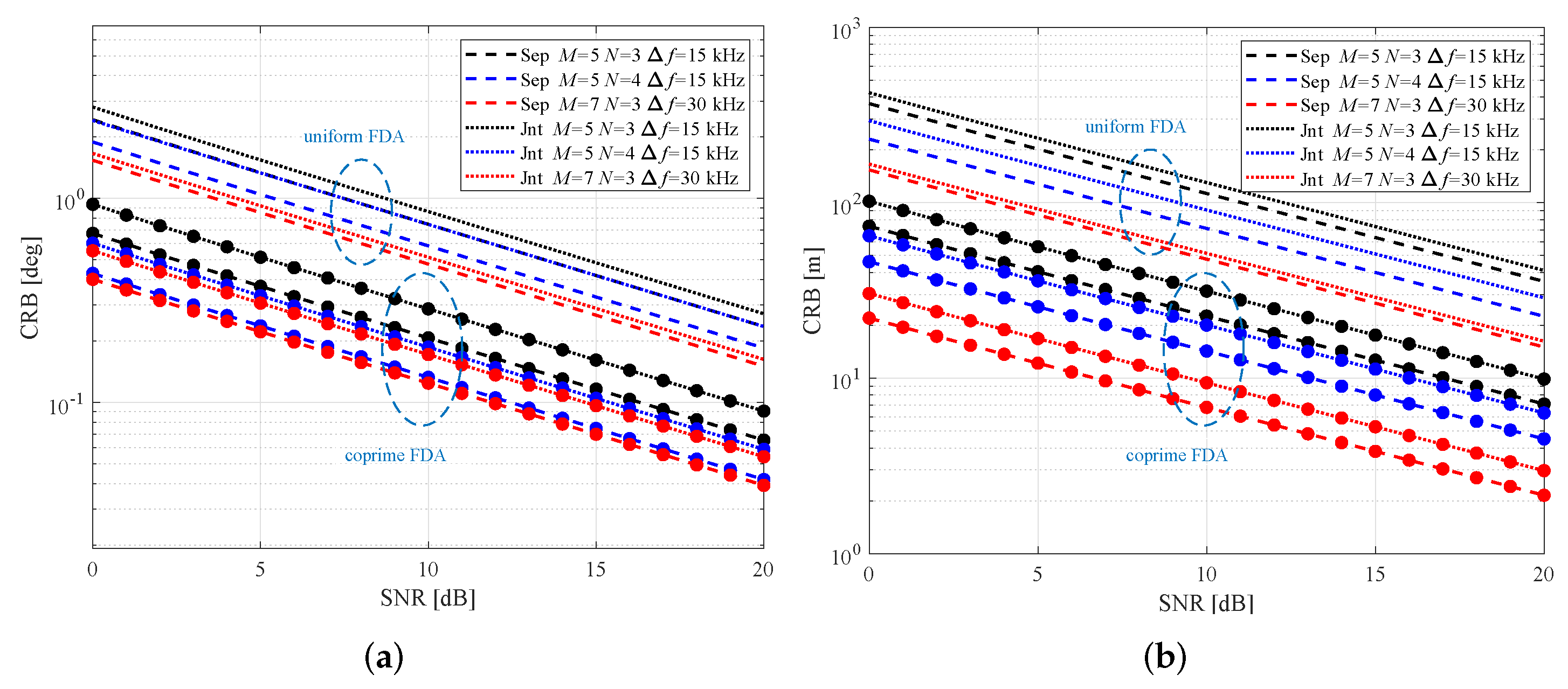
In this section, numerical simulations are presented to exemplify the CRBs in different scenarios. We assume that the coprime FDA under investigation operates at the X-band with a carrier frequency of $f_0=10\mathrm{GHz}$. Both deterministic and stochastic signal cases are investigated in the simulations. The location of the deterministic and stochastic signal sources are set as $\mathit{\alpha }=\mathit{\xi }$, and the azimuth angle is ${30}^{\circ }$ while the range is 2.8 km. To observe and analyze the CRB of coprime FDA, the following commonly-used coprime designs are simulated as examples: (a) $M=5,N=3,\Delta f=15\mathrm{kHz}$; (b) $M=7,N=3,\Delta f=15\mathrm{kHz}$; (c) $M=5,N=4,\Delta f=15\mathrm{kHz}$; (d) $M=5,N=3,\Delta f=30\mathrm{kHz}$; (e) $M=7,N=3,\Delta f=30\mathrm{kHz}$; (f) $M=5,N=4,\Delta f=30\mathrm{kHz}$. Note that the CRB results can be easily extended to other parameter settings using the closed-form solutions. We also include the CRBs of uniform FDA-MIMO [49] with the same number of array sensors in the numerical analyses to demonstrate the benefits of coprime configuration. The markers on the curves are used to distinguish between the CRBs of coprime and uniform FDAs.

Figure 2 shows the results of deterministic ${\mathrm{CRB}}_{\theta }$ and stochastic ${\mathrm{CRB}}_{\psi }$ for joint estimation versus SNR. The zoomed-in view in Figure 2a,b indicates that the impact of the frequency increment values on the CRBs of DOA estimation is trivial. Figure 3 presents the curves of the deterministic ${\mathrm{CRB}}_r$ and stochastic ${\mathrm{CRB}}_l$ versus SNR. We can see from Figure 3 that, in both deterministic and stochastic cases, the CRBs of range estimation decrease with the increase of the coprime FDA parameters M, N, and $\Delta f$. Furthermore, in contrast to the DOA estimation, the range estimation performance is significantly influenced by the unit frequency increment $\Delta f$. As for the comparison between the coprime FDA and the uniform FDA-MIMO, we infer from the numerical results that the CRB of coprime FDA is more than $60\%$ which is lower than that of uniform FDA-MIMO owing to the coprime configuration. The CRB performance for the detection of signals with different statistical characteristics is evaluated in Figure 4. Three groups of array design are simulated for deterministic and stochastic signal models. The simulation results suggest that the deterministic CRB outperforms the stochastic one, which tallies with the common knowledge in array signal processing.

In the following, we investigate the variation of angle CRB with the increase of frequency increment $\Delta f$. A variable ${\partial }_{\mathrm{CRB}}$ is used to quantify the magnitude of the CRB variation, which is defined as

$$\begin{array}{c}\hfill {\partial }_{\mathrm{CRB}}\triangleq \frac{{\mathrm{CRB}}_B-{\mathrm{CRB}}_0}{{\mathrm{CRB}}_0},\end{array}$$

(61)

where ${\mathrm{CRB}}_0$ and ${\mathrm{CRB}}_B$ denote the CRB of DOA when bandwidth is 0 and B, respectively. We let B and $\kappa =B/f_0$ respectively denote the overall and relative bandwidth of the coprime FDA. To ensure that the narrow-band assumption of coprime FDA is met, we assume that $\kappa$ is confined to ≤0.1. As depicted in Figure 5a, CRBs of DOA estimation in stochastic signal case decline with the increase of $\Delta f$. The curves in Figure 5a also implies a non-monotonic dependence of the deterministic ${\mathrm{CRB}}_{\theta }$ on the bandwidth. From (32) we notice that $J_{\theta r}$ increases with the increase of $\Delta f$. Hence, the dependence between parameters in the joint estimation cases is stronger. As a result, deterministic ${\mathrm{CRB}}_{\theta }$ first decreases and then increases when the bandwidth reaches a certain level. Nevertheless, in the case of joint estimation of stochastic signals as shown in Figure 5b, this phenomenon is inconspicuous.

We compare the CRBs of separate and joint estimations under both deterministic and stochastic signal models, which are respectively given in Figure 6 and Figure 7. In addition, we examine the root mean square errors (RMSEs) of the classical spatial spectrum estimation algorithms including the two-dimensional MUltiple SIgnal Classification (2-D MUSIC) [50] and two-dimensional minimum variance distortionless response (2-D MVDR) [51], and compare them with the CRBs. We observe from Figure 8 that both the RMSEs of 2-D MUSIC and 2-D MVDR can approach the CRB gradually as SNR increases.

In addition to the analyses of the numerical results, from the analytical form expressions given in (33)–(35) and (58)–(60), we arrive at the following remarks.

• Deterministic ${\mathrm{CRB}}_r$ (${\mathrm{SCRB}}_r$) and stochastic ${\mathrm{CRB}}_l$ (${\mathrm{SCRB}}_l$) are independent of the range, meaning that the range of signal source has no influence on the CRB of range estimation from the premise that the path loss is not considered.
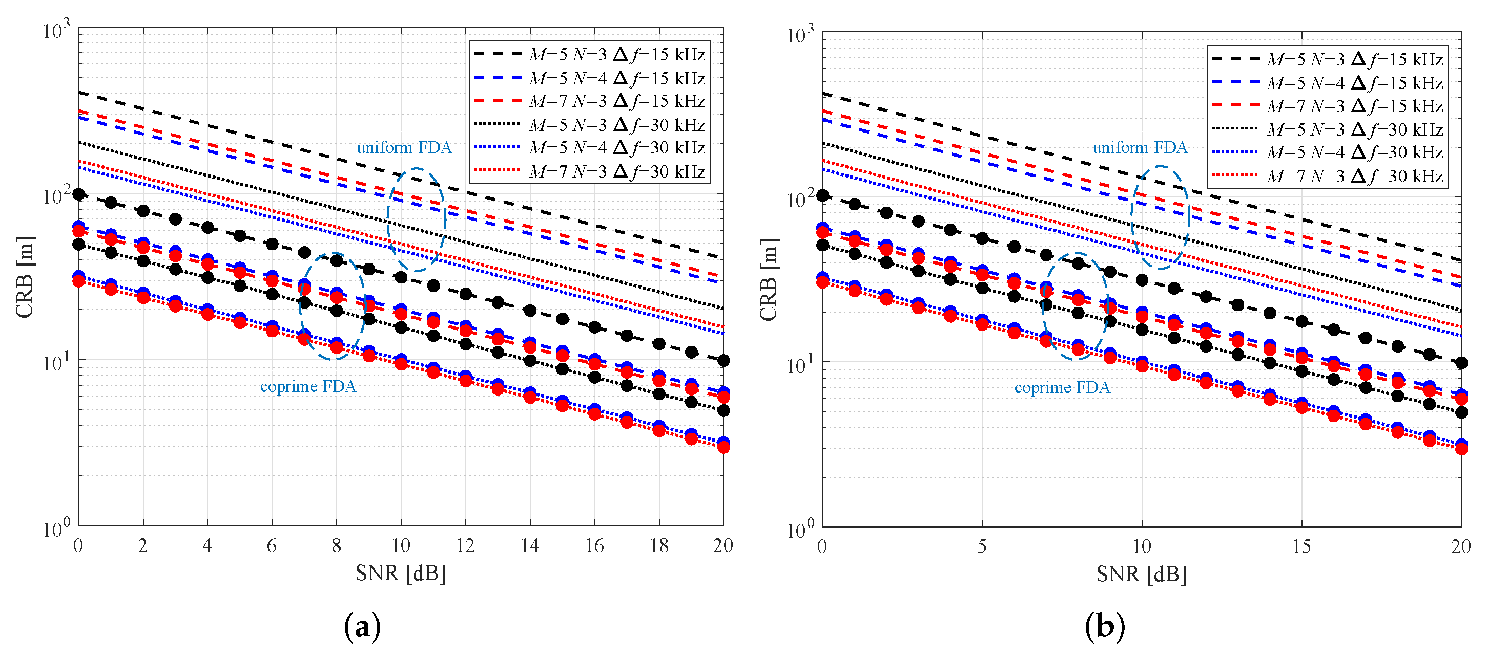
• Since a coprime FDA is narrow-band in nature, the frequency-increment-induced phase difference with respect to angle is much smaller than the array-spacing-induced one. As such, deterministic ${\mathrm{CRB}}_{\theta }$ and stochastic ${\mathrm{CRB}}_{\psi }$ are weakly dependent on the frequency increment $\Delta f$ (see Figure 2). This is, however, not the case for deterministic ${\mathrm{CRB}}_r$ (${\mathrm{SCRB}}_r$) and stochastic ${\mathrm{CRB}}_l$ (${\mathrm{SCRB}}_l$). Furthermore, the range estimation performance improves with the increase of the frequency increment (see Figure 3).
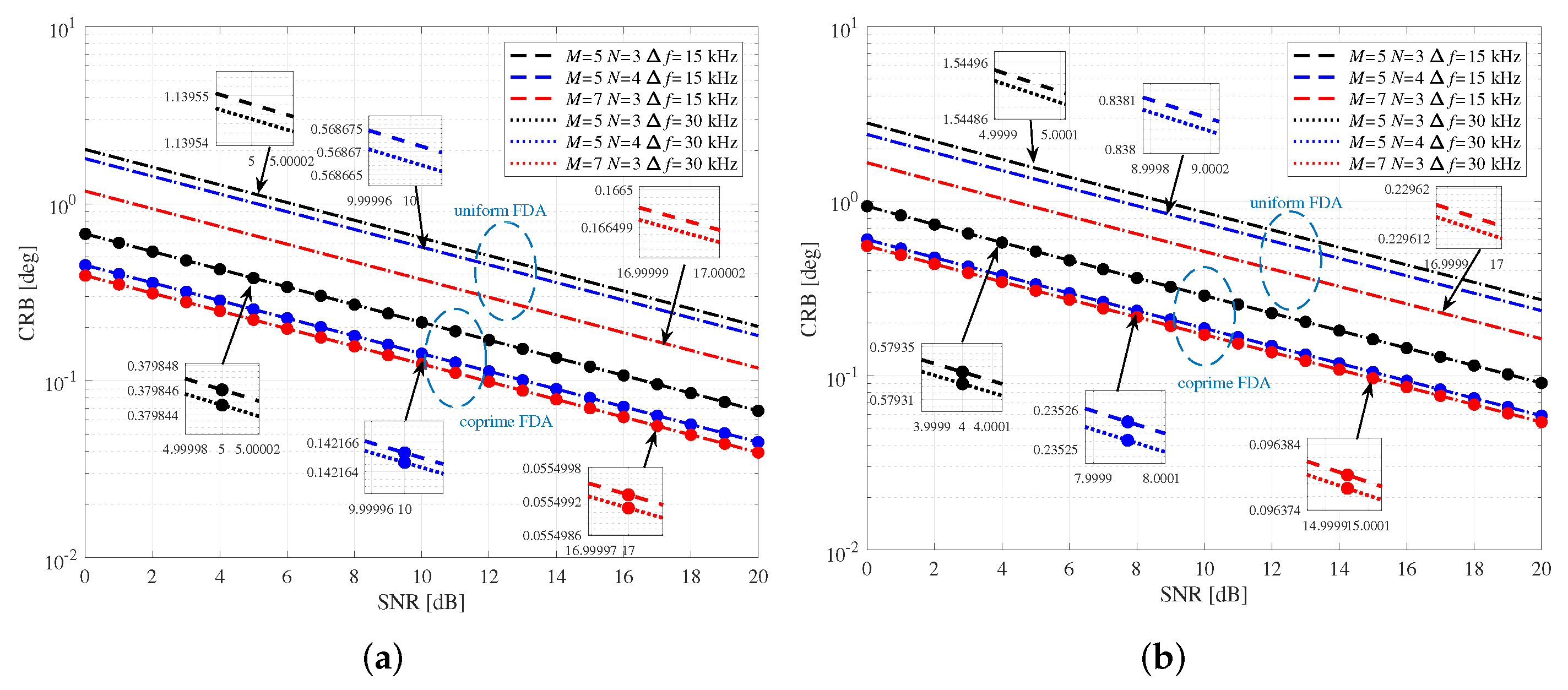
• Connecting to frequency increment $\Delta f$ has limited impact on the DOA estimation, and the dependence is not consistent in deterministic and stochastic CRBs for DOA estimation (see Figure 5). Connecting this phenomenon to the previous remark, the impact of $\Delta f$ on CRB for DOA estimation defies generalisations.
• For a sufficient number of sensors, deterministic ${\mathrm{CRB}}_{\theta }$, stochastic ${\mathrm{CRB}}_{\psi }$, deterministic ${\mathrm{CRB}}_r$ and stochastic ${\mathrm{CRB}}_l$ of coprime FDA are $\mathcal{O}(1/M^3{N}^3)$.
• The CRB of joint estimation is slightly worse than the SCRB. This implies that the prior knowledge on the range/DOA of target is conducive to improve measurement accuracy for deterministic and stochastic signal case (see Figure 6 and Figure 7).

Furthermore, we observe from Figure 2 that the CRBs of both DOA and range estimations decrease with the increase of coprime integers $M,N$, which leads to the expansion of array aperture and bandwidth. This result tallies with our common sense. Accordingly, we can use the largest $M,N$ possible to design a theoretically best-performance coprime FDA. Nevertheless, in reality, array designs are often subject to resource constraints such as the total number of antenna elements and/or bandwidth. Therefore, a rational design with limited resources is important in practice. From the analytical CRB results given in the above sections, we notice that a larger total number of antenna elements $M+N$ is not equivalent to superior CRB. The above conclusion is drawn in Figure 3a. More concretely, the CRB of range estimation for the coprime FDA choosing $M=5,N=4,\Delta f=15\mathrm{kHz}$, which uses a smaller number of elements, performs better than the coprime FDA choosing $M=7,N=3,\Delta f=15\mathrm{kHz}$. Based on this conclusion, we propose to use the CRB of coprime FDA to choose the optimal solution of coprime integers M and N to assist the array design.

Consider a practical scenario where the total number of antennas is L and the upper limit of bandwidth is $\tilde{B}$. By further denoting the coprime integers set as ${\mathbb{S}}_c$, we formulate the coprime FDA array design as the following optimization problem:

$$\begin{array}{cc}\hfill & \underset{M,N}{min}{\mathrm{CRB}}_{\theta }+\gamma ·{\mathrm{CRB}}_r,\hfill \\ \hfill & \mathrm{s}.\mathrm{t}.M+N\le L,\left(M-1\right)N·\Delta f\le \tilde{B},\hfill \\ \hfill & \{M,N\}\in {\mathbb{S}}_c,\hfill \end{array}$$

(62)

where $\gamma$ represents the trade-off coefficient that controls the compromise between the CRB of DOA (range) estimation. This problem can be readily solved via exhaustive search. In doing so, we are able to design a theoretically optimal coprime FDA configuration with constrained physical resources.

6. Conclusions

In this work, the analytical expressions of the CRBs in deterministic/stochastic signal cases for joint DOA-range estimation using coprime FDA are derived. Extensive numerical simulations are also provided and analyzed. We are able to arrive at the following conclusions from the simulation results: (i) The CRB of DOA estimation is weakly related with the frequency increment; (ii) The difference between the deterministic and stochastic CRBs is distinct; (iii) The relation between frequency increment and the CRB of DOA for joint estimation is nonmonotonic in the deterministic signal case; (iv) The CRB of joint DOA-range estimation is slightly worse than the separate parameter estimation in both the deterministic and stochastic signal cases; and (v) The CRB of coprime FDA outperforms that of uniform FDA-MIMO for more than $60\%$ under commonly-adopted coprime patterns. The difference between the CRBs of joint and separate DOA-range estimation methods is analyzed and we also propose an intuitive method for coprime FDA design based on CRB minimization.

References

1. Antonik, P.; Wicks, M.C.; Griffiths, H.D.; Baker, C.J. Range-dependent beamforming using element level waveform diversity. In Proceedings of the 2006 International Waveform Diversity & Design Conference, Las Vegas, NV, USA, 22–26 January 2006; pp. 140–144. [Google Scholar]
2. Antonik, P.; Wicks, M.C.; Griffiths, H.D.; Baker, C.J. Frequency diverse array radars. In Proceedings of the 2006 IEEE Conference on Radar, Verona, NY, USA, 24–27 April 2006; pp. 215–217. [Google Scholar]
3. Wang, W.-Q. Phased-MIMO radar with frequency diversity for range-dependent beamforming. IEEE Sens. J. 2013, 13, 1320–1328. [Google Scholar] [CrossRef]
4. Sammartino, P.F.; Baker, C.J.; Griffiths, H.D. Frequency diverse MIMO techniques for radar. IEEE Trans. Aerosp. Electron. Syst. 2013, 49, 1320–1328. [Google Scholar] [CrossRef]
5. Liao, Y.; Wang, W.; Zheng, Z. Frequency diverse array beampattern synthesis using symmetrical logarithmic frequency offsets for target indication. IEEE Trans. Antennas Propag. 2019, 67, 3505–3509. [Google Scholar] [CrossRef]
6. Wang, C.; Xu, J.; Liao, G.; Xu, X.; Zhang, Y. A range ambiguity resolution approach for high-resolution and wide-swath SAR imaging using frequency diverse array. IEEE J. Sel. Top. Signal Process. 2017, 11, 336–346. [Google Scholar] [CrossRef]
7. Lan, L.; Liao, G.; Xu, J.; Zhang, Y.; Liao, B. Transceive beamforming with accurate nulling in FDA-MIMO radar for imaging. IEEE Trans. Geosci. Remote Sens. 2020, 58, 4145–4159. [Google Scholar] [CrossRef]
8. Nusenu, S.Y.; Wang, W.-Q. Range-dependent spatial modulation using frequency diverse array for OFDM wireless communications. IEEE Trans. Veh. Technol. 2018, 67, 10886–10895. [Google Scholar] [CrossRef]
9. Wang, W.-Q. Range-angle dependent transmit beampattern synthesis for linear frequency diverse arrays. IEEE Trans. Antennas Propag. 2013, 61, 4073–4081. [Google Scholar] [CrossRef]
10. Secmen, M.; Demir, S.; Hizal, A.; Eker, T. Frequency diverse array antenna with periodic time modulated pattern in range and angle. In Proceedings of the 2007 IEEE Radar Conference, Boston, MA, USA, 17–20 April 2007; pp. 427–430. [Google Scholar]
11. Huang, S.; Tong, K.F.; Baker, C.J. Frequency diverse array: Simulation and design. In Proceedings of the 2009 Loughborough Antennas & Propagation Conference, Loughborough, UK, 16–17 November 2009; pp. 253–256. [Google Scholar]
12. Khan, W.; Qureshi, I.M. Frequency diverse array radar with time-dependent frequency offset. IEEE Antennas Wirel. Propag. Lett. 2014, 13, 758–761. [Google Scholar] [CrossRef]
13. Khan, W.; Qureshi, I.M.; Saeed, S. Frequency diverse array radar with logarithmically increasing frequency offset. IEEE Antennas Wirel. Propag. Lett. 2015, 14, 499–502. [Google Scholar] [CrossRef]
14. Mahmood, M.; Mir, H. Frequency diverse array beamforming using nonuniform logarithmic frequency increments. IEEE Antennas Wirel. Propag. Lett. 2018, 17, 1817–1821. [Google Scholar] [CrossRef]
15. Liu, Y.; Ruan, H.; Wang, L.; Nehorai, A. The random frequency diverse array: A new antenna structure for uncoupled direction-range indication in active sensing. IEEE J. Sel. Top. Signal Process. 2017, 11, 295–308. [Google Scholar] [CrossRef]
16. Wang, W.-Q.; So, H.C.; Shao, H. Nonuniform frequency diverse array for range-angle imaging of targets. IEEE Sens. J. 2014, 14, 2469–2476. [Google Scholar] [CrossRef]
17. Shao, H.; Li, J.; Chen, H.; Wang, W.-Q. Adaptive frequency offset selection in frequency diverse array radar. IEEE Antennas Wirel. Propag. Lett. 2014, 13, 1405–1408. [Google Scholar] [CrossRef]
18. Gao, K.; Wang, W.; Chen, H.; Cai, J. Transmit beamspace design for multi-carrier frequency diverse array sensor. IEEE Sens. J. 2016, 16, 5709–5714. [Google Scholar] [CrossRef]
19. Shao, H.; Dai, J.; Xiong, J.; Chen, H.; Wang, W.-Q. Dot-shaped range-angle beampattern synthesis for frequency diverse array. IEEE Antennas Wirel. Propag. Lett. 2016, 15, 1703–1706. [Google Scholar] [CrossRef]
20. Wang, Y.; Wang, W.-Q.; Chen, H.; Shao, H. Optimal frequency diverse subarray design with Cramér-Rao lower bound minimization. IEEE Antennas Wirel. Propag. Lett. 2015, 14, 1188–1191. [Google Scholar] [CrossRef]
21. Xiong, J.; Wang, W.-Q.; Shao, H.; Chen, H. Frequency diverse array transmit beampattern optimization with genetic algorithm. IEEE Antennas Wirel. Propag. Lett. 2017, 16, 469–472. [Google Scholar] [CrossRef]
22. Yang, Y.-Q.; Wang, H.-Q.; Wang, H.; Gu, S.-Q.; Xu, D.-L.; Quan, S.-L. Optimization of sparse frequency diverse array with time-invariant spatial-focusing beampattern. IEEE Antennas Wirel. Propag. Lett. 2018, 17, 351–354. [Google Scholar] [CrossRef]
23. Xu, J.; Liao, G.; Zhu, S.; Huang, L.; So, H.C. Joint range and angle estimation using MIMO radar with frequency diverse array. IEEE Trans. Signal Process. 2015, 63, 3396–3410. [Google Scholar] [CrossRef]
24. Wang, Y.; Huang, G.; Li, W. Transmit beampattern design in range and angle domains for MIMO frequency diverse array radar. IEEE Antennas Wirel. Propag. Lett. 2016, 16, 1003–1006. [Google Scholar] [CrossRef]
25. Li, J.; Stoica, P. MIMO radar with colocated antennas. IEEE Signal Process. Mag. 2007, 24, 106–114. [Google Scholar] [CrossRef]
26. BouDaher, E.; Jia, Y.; Ahmad, F.; Amin, M.G. Multi-frequency co-prime arrays for high-resolution direction-of-arrival estimation. IEEE Trans. Signal Process. 2015, 63, 3797–3808. [Google Scholar] [CrossRef]
27. Zheng, H.; Shi, Z.; Zhou, C.; Haardt, M.; Chen, J. Coupled coarray tensor CPD for DOA estimation with coprime L-shaped array. IEEE Signal Process. Lett. 2021, 28, 1545–1549. [Google Scholar] [CrossRef]
28. Qin, S.; Zhang, Y.D.; Amin, M.G. Generalized coprime array configurations for direction-of-arrival estimation. IEEE Trans. Signal Process. 2015, 63, 1377–1390. [Google Scholar] [CrossRef]
29. Vaidyanathan, P.P.; Pal, P. Sparse sensing with co-prime samplers and arrays. IEEE Trans. Signal Process. 2011, 59, 573–586. [Google Scholar] [CrossRef]
30. Qin, S.; Zhang, Y.D.; Amin, M.G.; Gini, F. Frequency diverse coprime arrays with coprime frequency offsets for multitarget localization. IEEE J. Sel. Top. Signal Process. 2017, 11, 321–335. [Google Scholar] [CrossRef]
31. Ahmed, A.; Zhang, Y.D. Generalized non-redundant sparse array designs. IEEE Trans. Signal Process. 2021, 69, 4580–4594. [Google Scholar] [CrossRef]
32. Zhou, C.; Gu, Y.; He, S.; Shi, Z. A robust and efficient algorithm for coprime array adaptive beamforming. IEEE Trans. Veh. Technol. 2018, 67, 1099–1122. [Google Scholar] [CrossRef]
33. Wang, W.-Q. Information geometry resolution optimization for frequency diverse array in DOA estimation. Digit. Signal Process. 2019, 44, 58–67. [Google Scholar] [CrossRef]
34. Liu, C.; Vaidyanathan, P.P. Cramér-Rao bounds for coprime and other sparse arrays, which find more sources than sensors. Digit. Signal Process. 2017, 61, 43–61. [Google Scholar] [CrossRef] [Green Version]
35. Xiong, J.; Wang, W.-Q.; Wang, Z. Optimization of frequency increments via CRLB minimization for frequency diverse array. In Proceedings of the 2017 IEEE Radar Conference, Seattle, WA, USA, 8–12 May 2017; pp. 645–650. [Google Scholar]
36. Stoica, P.; Nehorai, A. MUSIC, maximum likelihood and Cramer-Rao bound. In Proceedings of the International Conference on Acoustics, Speech, and Signal Processing, New York, NY, USA, 11–14 April 1988; pp. 2296–2299. [Google Scholar]
37. Zhou, C.; Gu, Y.; Fan, X.; Shi, Z.; Mao, G.; Zhang, Y.D. Direction-of-arrival estimation for coprime array via virtual array interpolation. IEEE Trans. Signal Process. 2018, 66, 5956–5971. [Google Scholar] [CrossRef]
38. Zhou, C.; Gu, Y.; Shi, Z.; Zhang, Y.D. Off-grid direction-of-arrival estimation using coprime array interpolation. IEEE Signal Process. Lett. 2018, 25, 1710–1714. [Google Scholar] [CrossRef]
39. Bekkerman, I.; Tabrikian, J. Target detection and localization using MIMO radars and sonars. IEEE Trans. Signal Process. 2006, 54, 3873–3883. [Google Scholar] [CrossRef]
40. Jiang, H.; Yi, W.; Kirubarajan, T.; Kong, L.; Yang, X. Multiframe radar detection of fluctuating targets using phase information. IEEE Trans. Aerosp. Electron. Syst. 2017, 53, 736–749. [Google Scholar] [CrossRef]
41. Kay, S. Waveform design for multistatic radar detection. IEEE Trans. Aerosp. Electron. Syst. 2009, 45, 1153–1166. [Google Scholar] [CrossRef]
42. Stoica, P.; Larsson, E.G.; Gershman, A.B. The stochastic CRB for array processing: A textbook derivation. IEEE Signal Process. Lett. 2001, 8, 148–150. [Google Scholar] [CrossRef]
43. Korso, M.N.E.; Boyer, R.; Renaux, A.; Marcos, S. Conditional and unconditional Cramér-Rao bounds for near-field source localization. IEEE Trans. Signal Process. 2010, 58, 2901–2907. [Google Scholar] [CrossRef]
44. Lebrun, J.; Comon, P. An algebraic approach to blind identification of communication channels. In Proceedings of the International Symposium on Signal Processing and Its Applications, Paris, France, 26 July 2003; pp. 665–668. [Google Scholar]
45. Trees, H.V. Detection, Estimation, and Modulation Theory, Optimum Array Processing; Wiley: Hoboken, NJ, USA, 2004. [Google Scholar]
46. Kumar, L.; Hegde, R.M. Stochastic Cramér-Rao bound analysis for DOA estimation in spherical harmonics domain. IEEE Signal Process. Lett. 2015, 22, 1030–1034. [Google Scholar] [CrossRef]
47. He, Q.; Blum, R.S.; Haimovich, A.M. Noncoherent MIMO radar for location and velocity estimation: More antennas means better performance. IEEE Trans. Signal Process. 2010, 58, 3661–3680. [Google Scholar] [CrossRef]
48. He, Q.; Blum, R.S. The significant gains from optimally processed multiple signals of opportunity and multiple receive stations in passive radar. IEEE Signal Process. Lett. 2014, 21, 180–184. [Google Scholar] [CrossRef]
49. Cong, J.; Wang, X.; Huang, M.; Bi, G. Feasible sparse spectrum fitting of DOA and range estimation for collocated FDA-MIMO radars. In Proceedings of the 2020 IEEE 11th Sensor Array and Multichannel Signal Processing Workshop (SAM), Hangzhou, China, 8–11 June 2020; pp. 1–5. [Google Scholar]
50. Xie, R.; Hu, D.; Luo, K.; Jiang, T. Performance analysis of joint range-velocity estimator with 2D-MUSIC in OFDM radar. IEEE Trans. Signal Process. 2021, 69, 4787–4800. [Google Scholar] [CrossRef]
51. Gu, Y.; Zhang, Y.D.; Goodman, N.A. Optimized compressive sensing-based direction-of-arrival estimation in massive MIMO. In Proceedings of the 2016 IEEE International Conference on Acoustics, Speech and Signal Processing (ICASSP), New Orleans, LA, USA, 20–25 March 2016; pp. 3181–3185. [Google Scholar]
Figure 1. Configuration of the coprime FDA under investigation.
Remotesensing 14 00583 g001
Figure 2. CRB of DOA in joint DOA-range estimation. (a) Deterministic signal case. (b) Stochastic signal case.
Remotesensing 14 00583 g002
Figure 3. CRB of range in joint DOA-range estimation. (a) Deterministic signal case. (b) Stochastic signal case.
Remotesensing 14 00583 g003
Figure 4. Comparison between two types of CRB. (a) CRB of DOA estimation in deterministic case and stochastic case. (b) CRB of range estimation in deterministic case and stochastic case.
Remotesensing 14 00583 g004
Figure 5. Influence of Δ f on the DOA estimation performance. (a) CRB θ and CRB ψ versus κ . (b) SCRB θ and SCRB ψ versus κ .
Remotesensing 14 00583 g005
Figure 6. CRBs of joint/separate DOA-range estimations in deterministic signal case. (a) CRB of DOA estimation. (b) CRB of range estimation.
Remotesensing 14 00583 g006
Figure 7. CRBs of joint/separate DOA-range estimations in stochastic signal case. (a) CRB of DOA estimation. (b) CRB of range estimation.
Remotesensing 14 00583 g007
Figure 8. RMSEs of 2-D MUSIC and 2-D MVDR algorithm. The coprime FDA parameters are set as M = 5 , N = 3 and Δ f = 15 kHz . The number of snapshots is set as 100 and the result is obtained through 500 Monte Carlo trials. (a) RMSE of DOA estimation. (b) RMSE of range estimation.
Remotesensing 14 00583 g008
Publisher’s Note: MDPI stays neutral with regard to jurisdictional claims in published maps and institutional affiliations.