
A Scale-Separating Framework for Fusing Satellite Land Surface Temperature Products


Abstract
:
1. Introduction
- To address the non-linearity of inter-sensor LST relationships with incorporation of a neural network,
- To capture temporal change in LST in multiple scales, and
- To generate high-quality fine resolution LST images in urban areas to support studies of intra-city temperature variations.
2. Materials and Methods
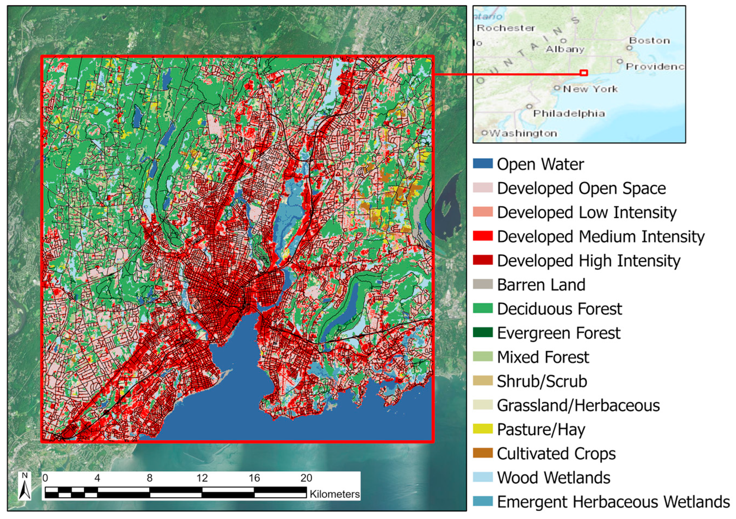
2.1. Study Area
2.2. LST Data
2.3. Sensor-to-Sensor Biases
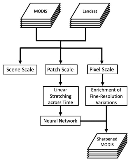
2.4. Framework Description
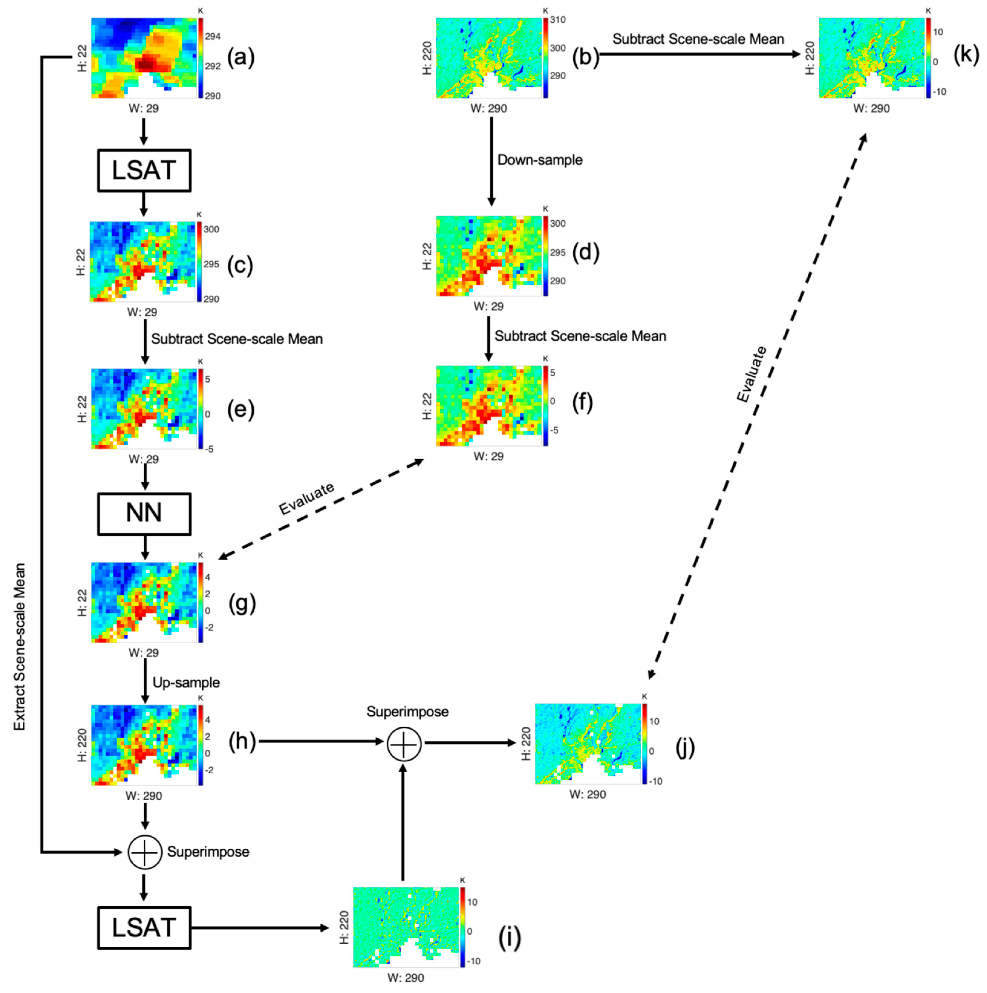
2.4.1. Workflow
2.4.2. Linear Stretching across Time (LSAT)
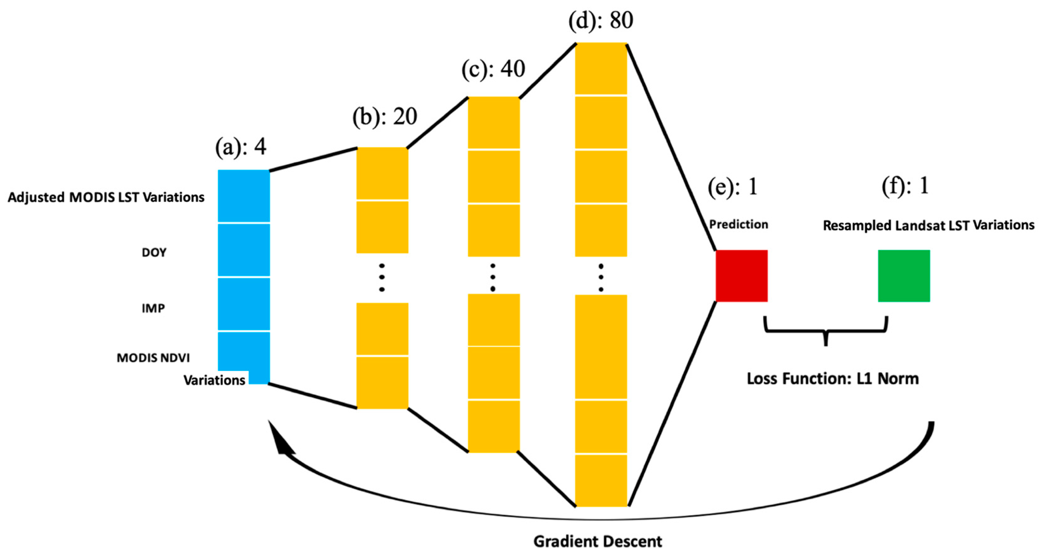
2.4.3. Neural Network
2.4.4. Enrichment of Fine-Resolution Variations
2.4.5. Sharpening an Arbitrary MODIS Image
3. Results
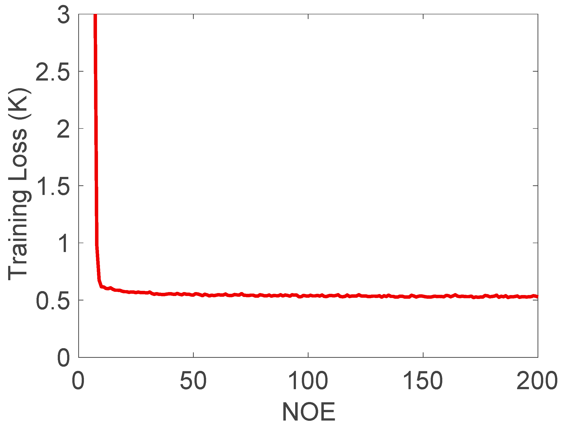
3.1. Training and Validation Loss
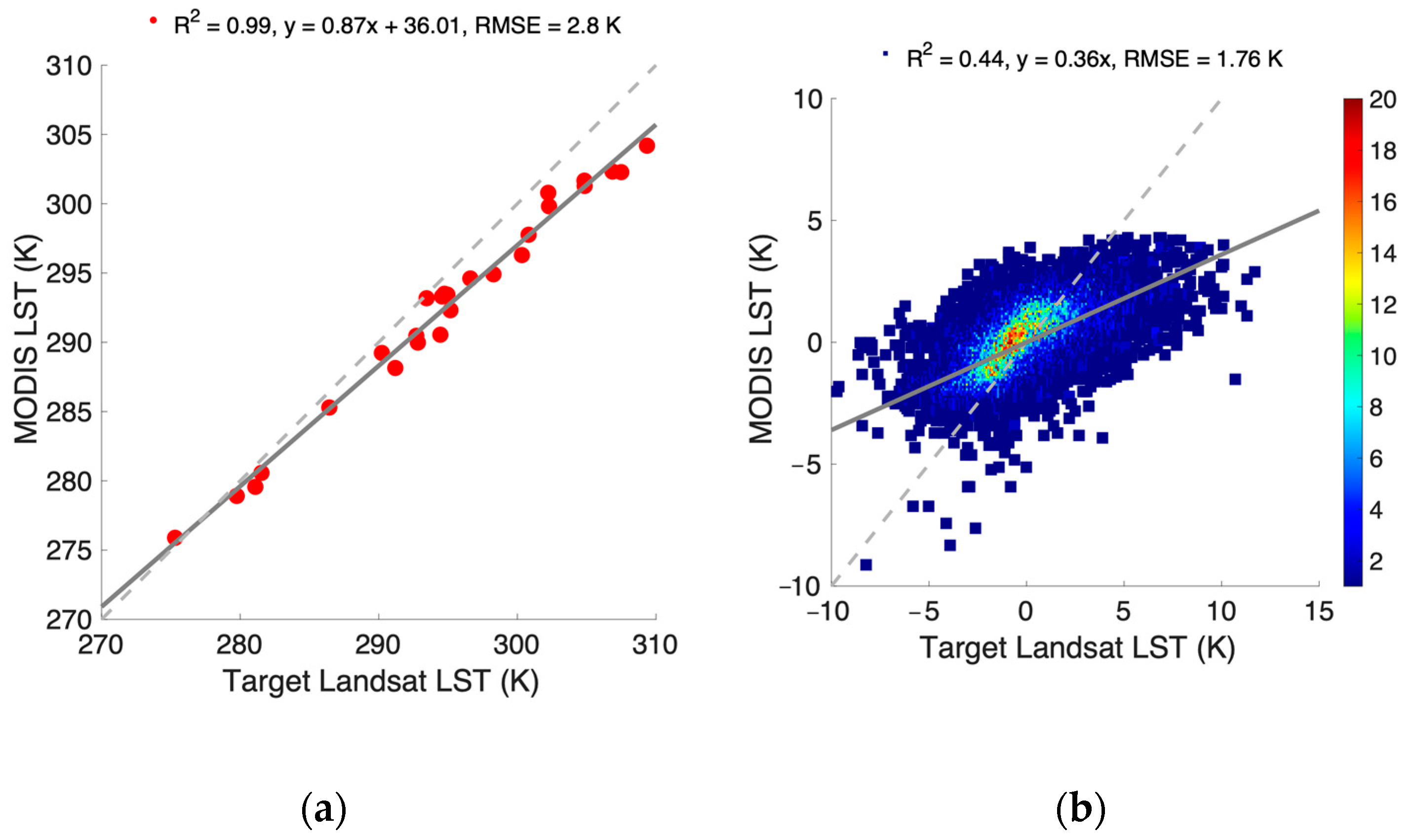
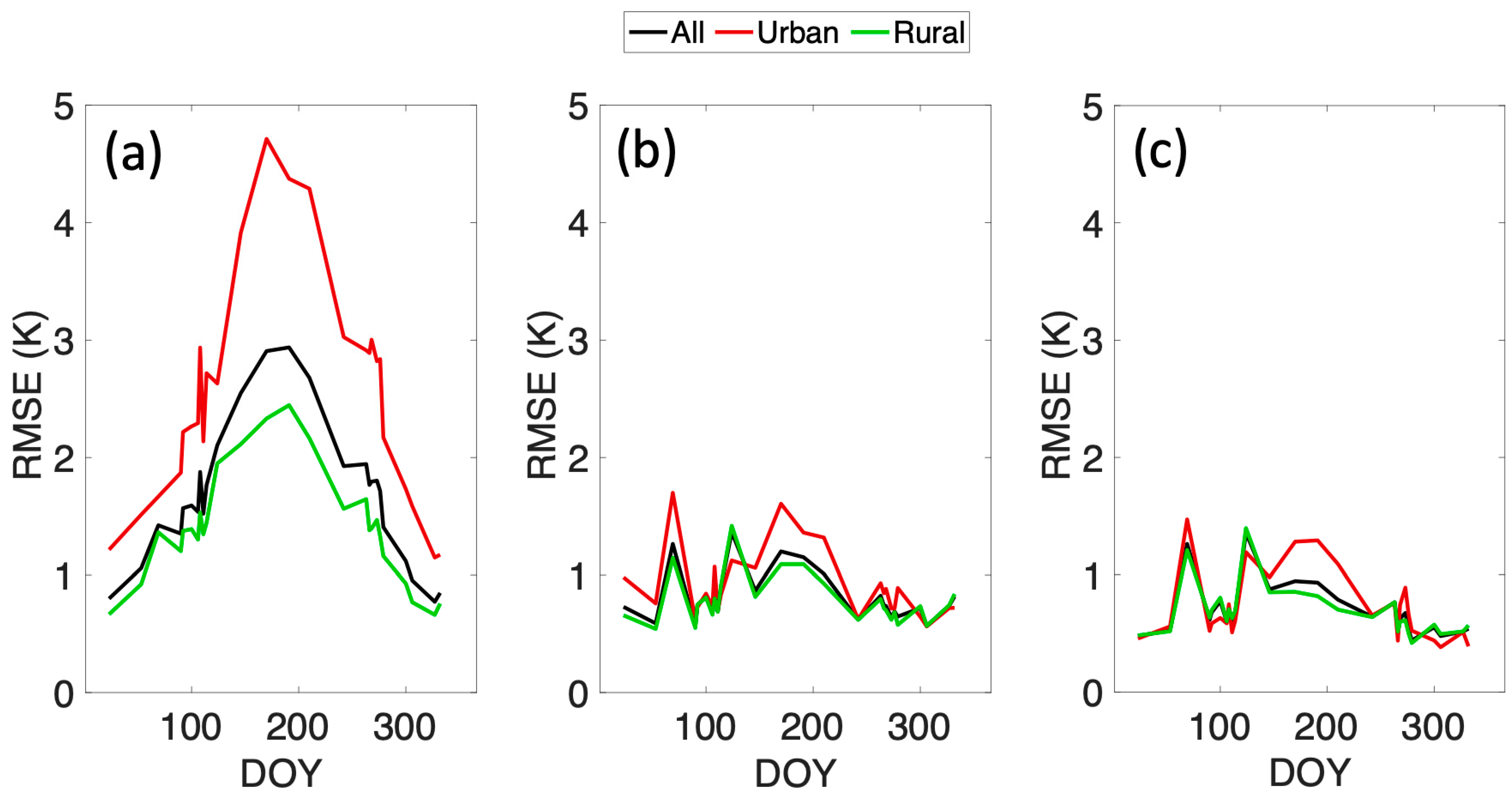
3.2. Accuracy Assessment
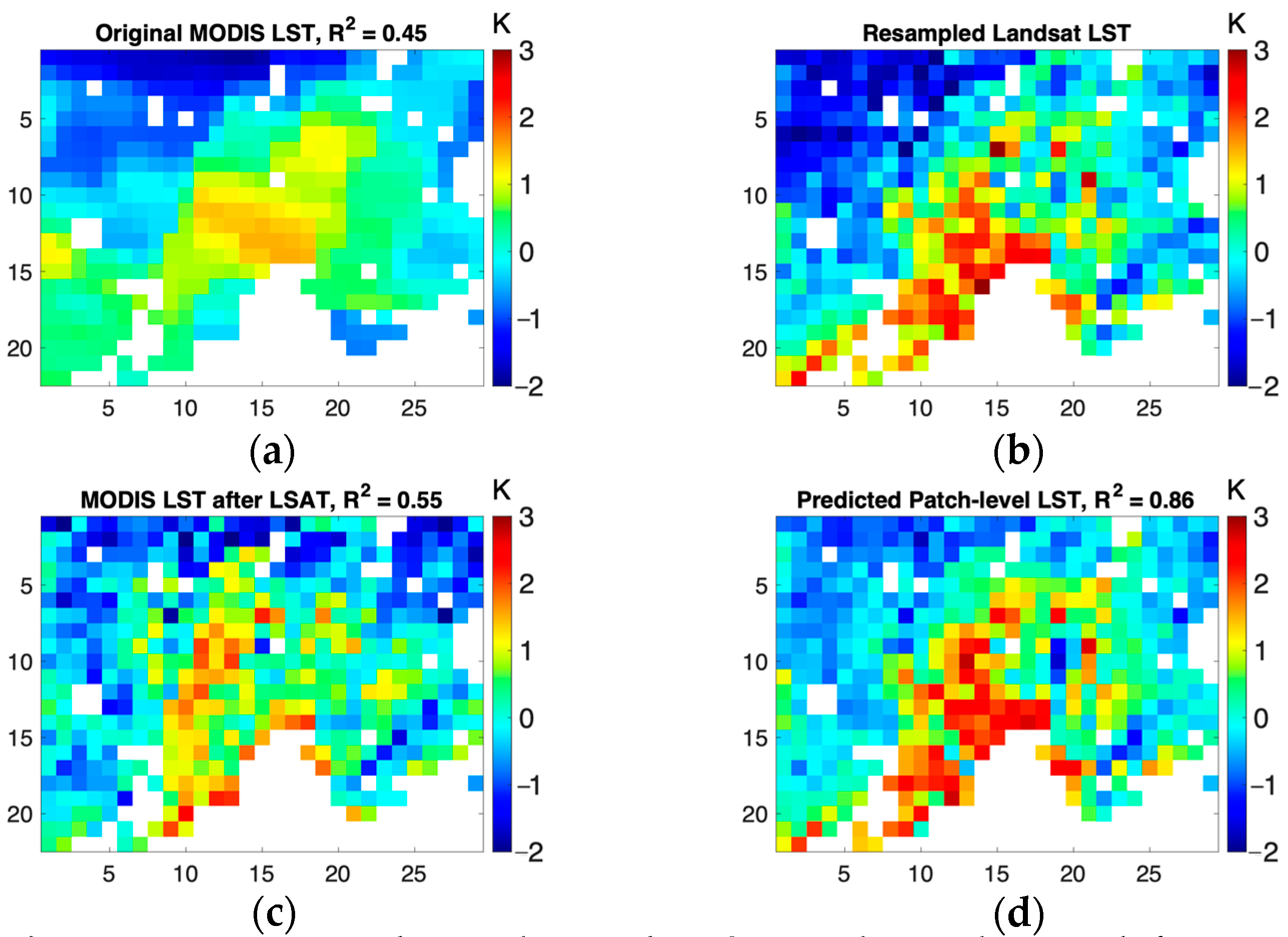
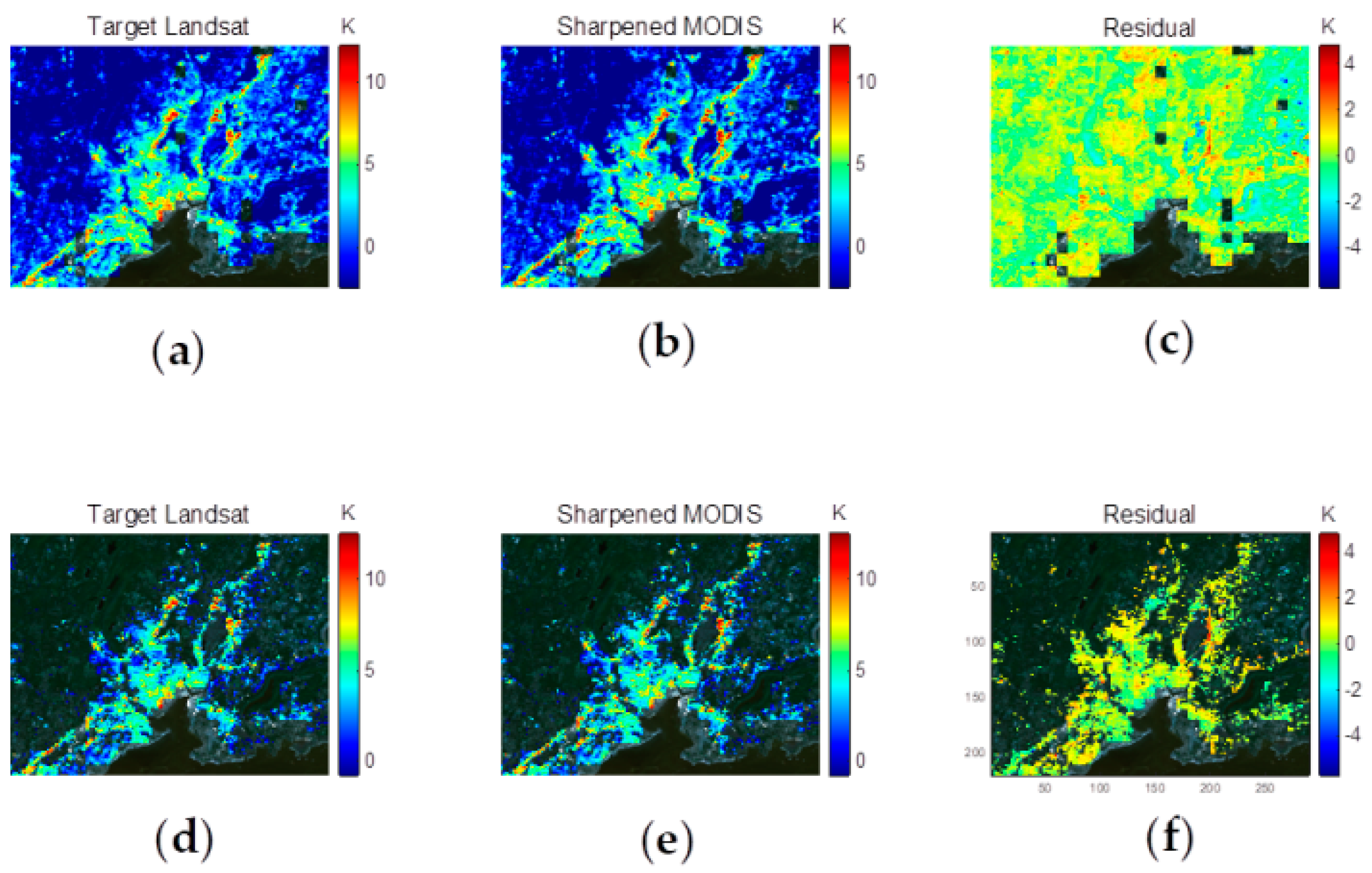
3.3. Evaluation of Sharpened LST
3.4. Comparison with Bilateral Filtering
4. Discussion
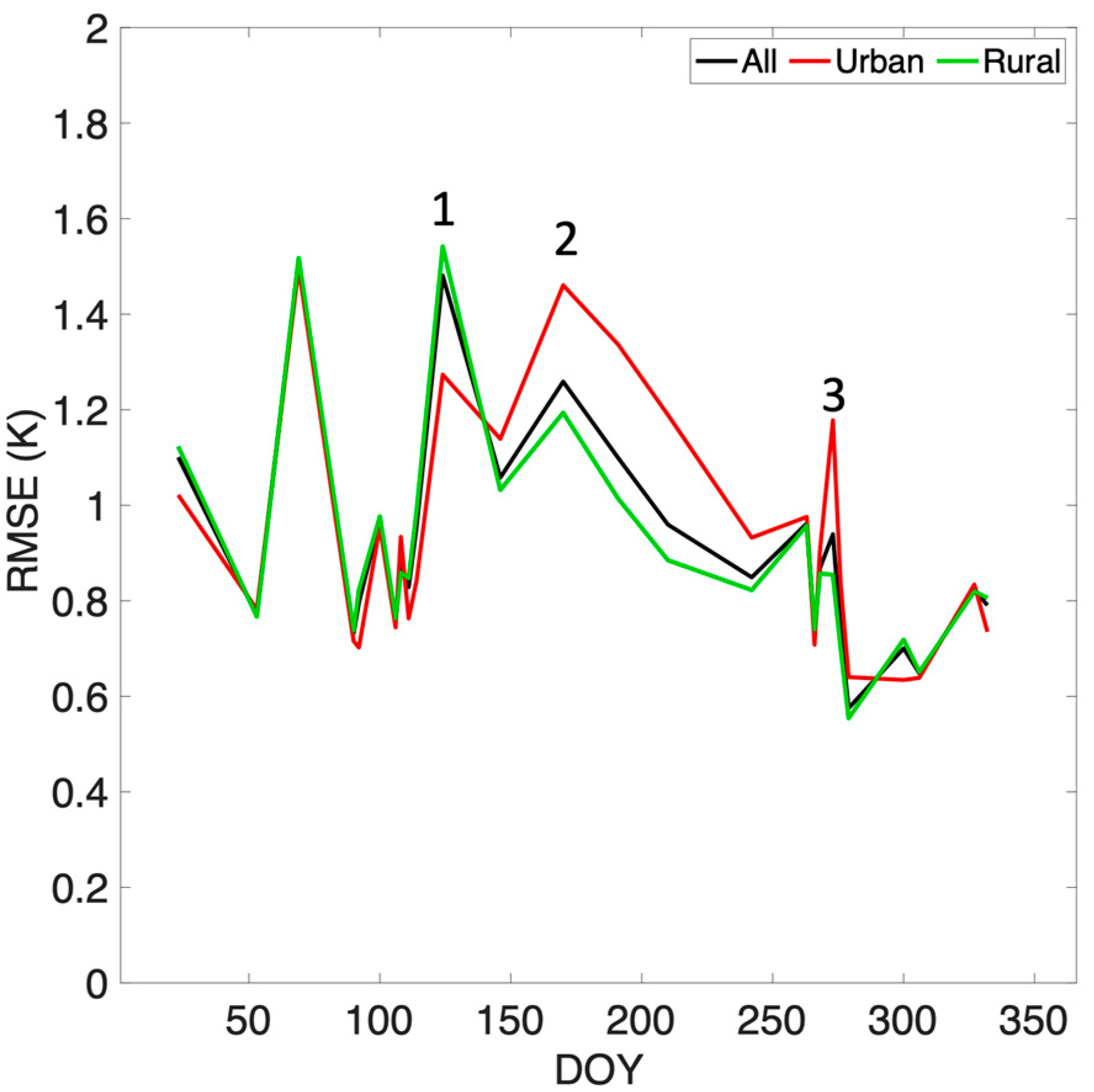
4.1. Error Analysis
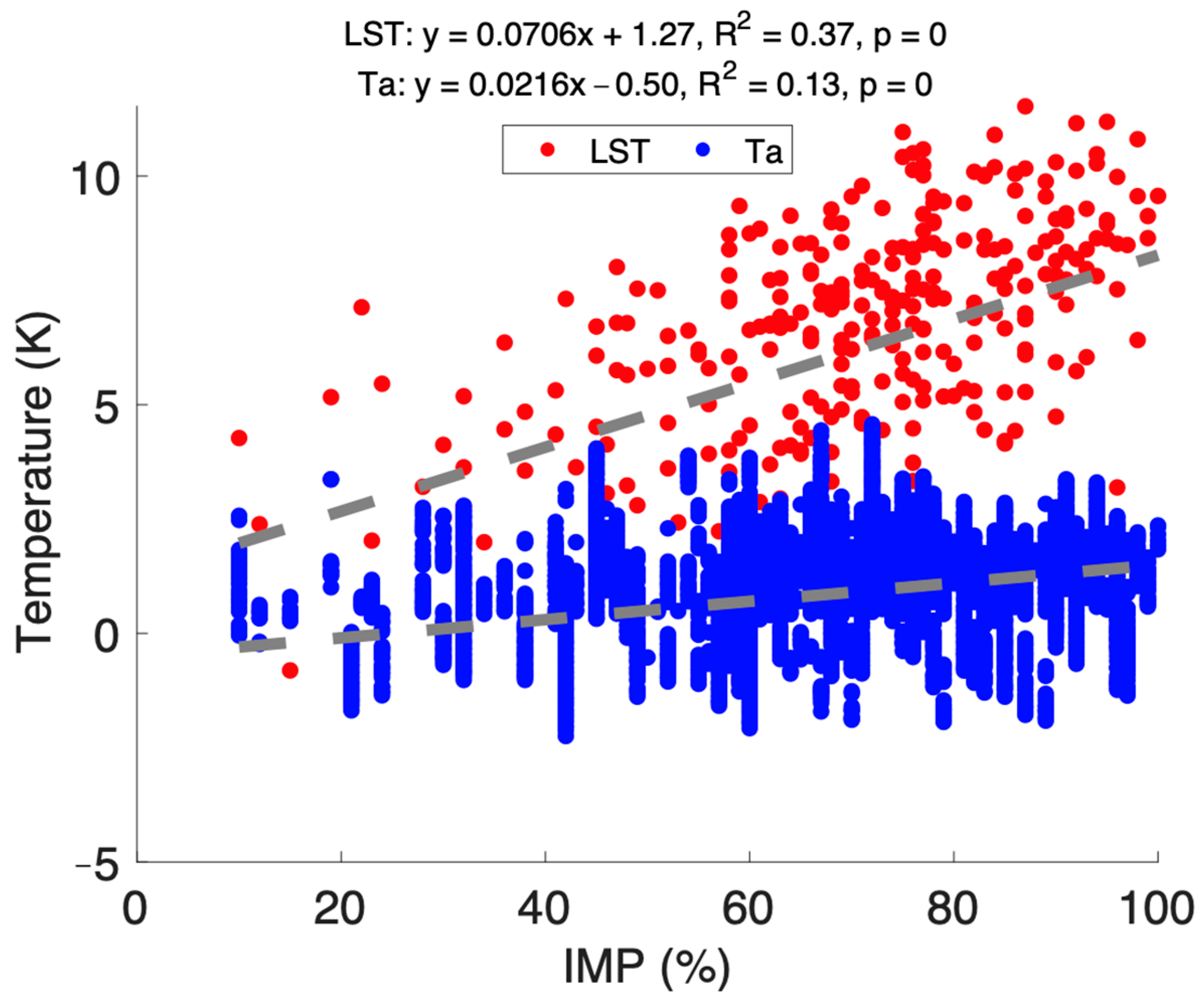
4.2. Comparison with Air Temperature
5. Conclusions
Supplementary Materials
Author Contributions
Funding
Data Availability Statement
Acknowledgments
Conflicts of Interest
References
- Oke, T.R. Boundary Layer Climates; Routledge: London, UK, 2002. [Google Scholar]
- Lee, X.; Goulden, M.L.; Hollinger, D.Y.; Barr, A.; Black, T.A.; Bohrer, G.; Bracho, R.; Drake, B.; Goldstein, A.; Gu, L. Observed increase in local cooling effect of deforestation at higher latitudes. Nature 2011, 479, 384–387. [Google Scholar] [CrossRef] [PubMed]
- Liu, Z.; Ballantyne, A.P.; Cooper, L.A. Biophysical feedback of global forest fires on surface temperature. Nat. Commun. 2019, 10, 214. [Google Scholar] [CrossRef] [PubMed] [Green Version]
- Maimaitiyiming, M.; Ghulam, A.; Tiyip, T.; Pla, F.; Latorre-Carmona, P.; Halik, Ü.; Sawut, M.; Caetano, M. Effects of green space spatial pattern on land surface temperature: Implications for sustainable urban planning and climate change adaptation. ISPRS J. Photogramm. Remote Sens. 2014, 89, 59–66. [Google Scholar] [CrossRef] [Green Version]
- Meehl, G.A. Influence of the land surface in the asian summer monsoon: External conditions versus internal feedbacks. J. Clim. 1994, 7, 1033–1049. [Google Scholar] [CrossRef] [Green Version]
- Bastiaanssen, W.G.; Menenti, M.; Feddes, R.; Holtslag, A. A remote sensing surface energy balance algorithm for land (sebal). 1. Formulation. J. Hydrol. 1998, 212, 198–212. [Google Scholar] [CrossRef]
- Jackson, R.; Reginato, R.; Idso, S. Wheat canopy temperature: A practical tool for evaluating water requirements. Water Resour. Res. 1977, 13, 651–656. [Google Scholar] [CrossRef]
- Chuvieco, E.; Cocero, D.; Riano, D.; Martin, P.; Martınez-Vega, J.; de la Riva, J.; Pérez, F. Combining ndvi and surface temperature for the estimation of live fuel moisture content in forest fire danger rating. Remote Sens. Environ. 2004, 92, 322–331. [Google Scholar] [CrossRef]
- Guangmeng, G.; Mei, Z. Using modis land surface temperature to evaluate forest fire risk of northeast china. IEEE Geosci. Remote Sens. Lett. 2004, 1, 98–100. [Google Scholar] [CrossRef]
- Schmugge, T.J.; André, J.-C. Land Surface Evaporation: Measurement and Parameterization; Springer Science & Business Media: Berlin, Germany, 2012. [Google Scholar]
- Zink, M.; Mai, J.; Cuntz, M.; Samaniego, L. Conditioning a hydrologic model using patterns of remotely sensed land surface temperature. Water Resour. Res. 2018, 54, 2976–2998. [Google Scholar] [CrossRef]
- Raynolds, M.K.; Comiso, J.C.; Walker, D.A.; Verbyla, D. Relationship between satellite-derived land surface temperatures, arctic vegetation types, and ndvi. Remote Sens. Environ. 2008, 112, 1884–1894. [Google Scholar] [CrossRef]
- Sims, D.A.; Rahman, A.F.; Cordova, V.D.; El-Masri, B.Z.; Baldocchi, D.D.; Bolstad, P.V.; Flanagan, L.B.; Goldstein, A.H.; Hollinger, D.Y.; Misson, L. A new model of gross primary productivity for north american ecosystems based solely on the enhanced vegetation index and land surface temperature from modis. Remote Sens. Environ. 2008, 112, 1633–1646. [Google Scholar] [CrossRef]
- Connors, J.P.; Galletti, C.S.; Chow, W.T. Landscape configuration and urban heat island effects: Assessing the relationship between landscape characteristics and land surface temperature in phoenix, arizona. Landsc. Ecol. 2013, 28, 271–283. [Google Scholar] [CrossRef]
- Kumar, K.S.; Bhaskar, P.U.; Padmakumari, K. Estimation of land surface temperature to study urban heat island effect using landsat etm+ image. Int. J. Eng. Sci. Technol. 2012, 4, 771–778. [Google Scholar]
- Zhao, L.; Lee, X.; Smith, R.B.; Oleson, K. Strong contributions of local background climate to urban heat islands. Nature 2014, 511, 216–219. [Google Scholar] [CrossRef]
- Yin, Z.; Wu, P.; Foody, G.M.; Wu, Y.; Liu, Z.; Du, Y.; Ling, F. Spatiotemporal fusion of land surface temperature based on a convolutional neural network. IEEE Trans. Geosci. Remote Sens. 2020, 59, 1808–1822. [Google Scholar] [CrossRef]
- Song, H.; Liu, Q.; Wang, G.; Hang, R.; Huang, B. Spatiotemporal satellite image fusion using deep convolutional neural networks. IEEE J. Sel. Top. Appl. Earth Obs. Remote Sens. 2018, 11, 821–829. [Google Scholar] [CrossRef]
- Zhan, W.; Chen, Y.; Zhou, J.; Wang, J.; Liu, W.; Voogt, J.; Zhu, X.; Quan, J.; Li, J. Disaggregation of remotely sensed land surface temperature: Literature survey, taxonomy, issues, and caveats. Remote Sens. Environ. 2013, 131, 119–139. [Google Scholar] [CrossRef]
- Zhan, W.; Chen, Y.; Zhou, J.; Li, J.; Liu, W. Sharpening thermal imageries: A generalized theoretical framework from an assimilation perspective. IEEE Trans. Geosci. Remote Sens. 2010, 49, 773–789. [Google Scholar] [CrossRef]
- Kustas, W.P.; Norman, J.M.; Anderson, M.C.; French, A.N. Estimating subpixel surface temperatures and energy fluxes from the vegetation index–radiometric temperature relationship. Remote Sens. Environ. 2003, 85, 429–440. [Google Scholar] [CrossRef]
- Agam, N.; Kustas, W.P.; Anderson, M.C.; Li, F.; Neale, C.M. A vegetation index based technique for spatial sharpening of thermal imagery. Remote Sens. Environ. 2007, 107, 545–558. [Google Scholar] [CrossRef]
- Essa, W.; Verbeiren, B.; van der Kwast, J.; Van de Voorde, T.; Batelaan, O. Evaluation of the distrad thermal sharpening methodology for urban areas. Int. J. Appl. Earth Obs. Geoinf. 2012, 19, 163–172. [Google Scholar] [CrossRef]
- Pan, X.; Zhu, X.; Yang, Y.; Cao, C.; Zhang, X.; Shan, L. Applicability of downscaling land surface temperature by using normalized difference sand index. Sci. Rep. 2018, 8, 9530. [Google Scholar] [CrossRef] [PubMed] [Green Version]
- Gao, F.; Masek, J.; Schwaller, M.; Hall, F. On the blending of the landsat and modis surface reflectance: Predicting daily landsat surface reflectance. IEEE Trans. Geosci. Remote Sens. 2006, 44, 2207–2218. [Google Scholar]
- Zhu, X.; Chen, J.; Gao, F.; Chen, X.; Masek, J.G. An enhanced spatial and temporal adaptive reflectance fusion model for complex heterogeneous regions. Remote Sens. Environ. 2010, 114, 2610–2623. [Google Scholar] [CrossRef]
- Huang, B.; Wang, J.; Song, H.; Fu, D.; Wong, K. Generating high spatiotemporal resolution land surface temperature for urban heat island monitoring. IEEE Geosci. Remote Sens. Lett. 2013, 10, 1011–1015. [Google Scholar] [CrossRef]
- Wu, P.; Shen, H.; Zhang, L.; Göttsche, F.-M. Integrated fusion of multi-scale polar-orbiting and geostationary satellite observations for the mapping of high spatial and temporal resolution land surface temperature. Remote Sens. Environ. 2015, 156, 169–181. [Google Scholar] [CrossRef]
- Quan, J.; Zhan, W.; Ma, T.; Du, Y.; Guo, Z.; Qin, B. An integrated model for generating hourly landsat-like land surface temperatures over heterogeneous landscapes. Remote Sens. Environ. 2018, 206, 403–423. [Google Scholar] [CrossRef]
- Quan, J.; Chen, Y.; Zhan, W.; Wang, J.; Voogt, J.; Li, J. A hybrid method combining neighborhood information from satellite data with modeled diurnal temperature cycles over consecutive days. Remote Sens. Environ. 2014, 155, 257–274. [Google Scholar] [CrossRef]
- Quan, J.; Zhan, W.; Chen, Y.; Wang, M.; Wang, J. Time series decomposition of remotely sensed land surface temperature and investigation of trends and seasonal variations in surface urban heat islands. J. Geophys. Res. Atmos. 2016, 121, 2638–2657. [Google Scholar] [CrossRef]
- Cook, M.; Schott, J.R.; Mandel, J.; Raqueno, N. Development of an operational calibration methodology for the landsat thermal data archive and initial testing of the atmospheric compensation component of a land surface temperature (lst) product from the archive. Remote Sens. 2014, 6, 11244–11266. [Google Scholar] [CrossRef] [Green Version]
- Cook, M.J. Atmospheric Compensation for a Landsat Land Surface Temperature Product; Rochester Institute of Technology: New York, NY, USA, 2014. [Google Scholar]
- Malakar, N.K.; Hulley, G.C.; Hook, S.J.; Laraby, K.; Cook, M.; Schott, J.R. An operational land surface temperature product for landsat thermal data: Methodology and validation. IEEE Trans. Geosci. Remote Sens. 2018, 56, 5717–5735. [Google Scholar] [CrossRef]
- Snyder, W.C.; Wan, Z.; Zhang, Y.; Feng, Y.Z. Classification-based emissivity for land surface temperature measurement from space. Int. J. Remote Sens. 1998, 19, 2753–2774. [Google Scholar] [CrossRef]
- Chakraborty, T.C.; Lee, X.; Ermida, S.; Zhan, W. On the land emissivity assumption and landsat-derived surface urban heat islands: A global analysis. Remote Sens. Environ. 2021, 265, 112682. [Google Scholar] [CrossRef]
- Wan, Z. Modis Land Surface Temperature Products Users’ Guide; Institute for Computational Earth System Science, University of California: Santa Barbara, CA, USA, 2006. [Google Scholar]
- Hu, L.; Monaghan, A.; Voogt, J.A.; Barlage, M. A first satellite-based observational assessment of urban thermal anisotropy. Remote Sens. Environ. 2016, 181, 111–121. [Google Scholar] [CrossRef] [Green Version]
- Krayenhoff, E.S.; Voogt, J.A. Daytime thermal anisotropy of urban neighbourhoods: Morphological causation. Remote Sens. 2016, 8, 108. [Google Scholar] [CrossRef] [Green Version]
- Cao, C.; Yang, Y.; Lu, Y.; Schultze, N.; Gu, P.; Zhou, Q.; Xu, J.; Lee, X. Performance evaluation of a smart mobile air temperature and humidity sensor for characterizing intracity thermal environment. J. Atmos. Ocean. Technol. 2020, 37, 1891–1905. [Google Scholar] [CrossRef]
- Li, H.; Wolter, M.; Wang, X.; Sodoudi, S. Impact of land cover data on the simulation of urban heat island for berlin using wrf coupled with bulk approach of noah-lsm. Theor. Appl. Climatol. 2018, 134, 67–81. [Google Scholar] [CrossRef]
- Li, H.; Zhou, Y.; Wang, X.; Zhou, X.; Zhang, H.; Sodoudi, S. Quantifying urban heat island intensity and its physical mechanism using wrf/ucm. Sci. Total Environ. 2019, 650, 3110–3119. [Google Scholar] [CrossRef]
- Yuan, F.; Bauer, M.E. Comparison of impervious surface area and normalized difference vegetation index as indicators of surface urban heat island effects in landsat imagery. Remote Sens. Environ. 2007, 106, 375–386. [Google Scholar] [CrossRef]
- Ziter, C.D.; Pedersen, E.J.; Kucharik, C.J.; Turner, M.G. Scale-dependent interactions between tree canopy cover and impervious surfaces reduce daytime urban heat during summer. Proc. Natl. Acad. Sci. USA 2019, 116, 7575–7580. [Google Scholar] [CrossRef] [Green Version]
- Li, D.; Liao, W.; Rigden, A.J.; Liu, X.; Wang, D.; Malyshev, S.; Shevliakiva, E. Urban heat island: Aerodynamics or imperviousness? Sci. Adv. 2019, 5, eaau4299. [Google Scholar] [CrossRef] [Green Version]
- Yap, D.; Oke, T.R. Sensible heat fluxes over an urban area—Vancouver, BC. J. Appl. Meteorol. Climatol. 1974, 13, 880–890. [Google Scholar] [CrossRef] [Green Version]
- Kato, S.; Yamaguchi, Y. Analysis of urban heat-island effect using ASTER and ETM+ Data: Separation of anthropogenic heat discharge and natural heat radiation from sensible heat flux. Remote Sens. Environ. 2005, 99, 44–54. [Google Scholar] [CrossRef]
- Li, H.; Zhou, Y.; Li, X.; Meng, L.; Wang, X.; Wu, S.; Sodoudi, S. A new method to quantify surface urban heat island intensity. Sci. Total Environ. 2018, 624, 262–272. [Google Scholar] [CrossRef] [PubMed]


Publisher’s Note: MDPI stays neutral with regard to jurisdictional claims in published maps and institutional affiliations. |
© 2022 by the authors. Licensee MDPI, Basel, Switzerland. This article is an open access article distributed under the terms and conditions of the Creative Commons Attribution (CC BY) license (https://creativecommons.org/licenses/by/4.0/).
Share and Cite
Yang, Y.; Lee, X. A Scale-Separating Framework for Fusing Satellite Land Surface Temperature Products. Remote Sens. 2022, 14, 983. https://doi.org/10.3390/rs14040983
Yang Y, Lee X. A Scale-Separating Framework for Fusing Satellite Land Surface Temperature Products. Remote Sensing. 2022; 14(4):983. https://doi.org/10.3390/rs14040983
Chicago/Turabian StyleYang, Yichen, and Xuhui Lee. 2022. "A Scale-Separating Framework for Fusing Satellite Land Surface Temperature Products" Remote Sensing 14, no. 4: 983. https://doi.org/10.3390/rs14040983
APA StyleYang, Y., & Lee, X. (2022). A Scale-Separating Framework for Fusing Satellite Land Surface Temperature Products. Remote Sensing, 14(4), 983. https://doi.org/10.3390/rs14040983