Figure 1.
Illustration of semantic segmentation results obtained using the baseline model on the SpaceNet building dataset: (a) Khartoum and (b) Las Vegas. One problem with convolutional neural network (CNN)-based building extraction methods is that the boundaries of the buildings tend to be blurred, with most boundary pixels belonging to the category of interest being misclassified as background pixels.
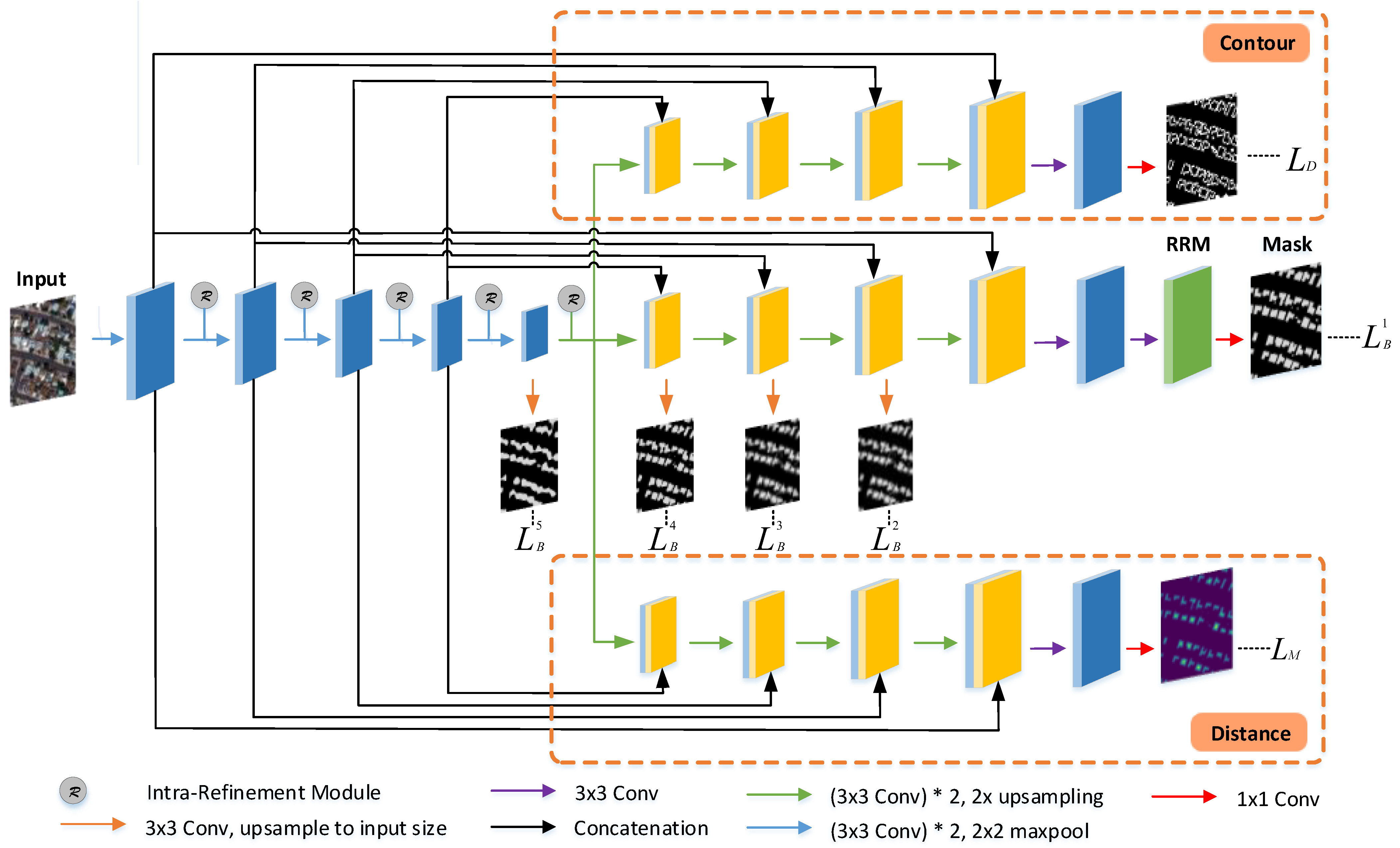
Figure 2.
Overview of the proposed model. The encoder applies repeated downsampling operations, each of which is followed by an intra-refinement module, and three decoders perform different tasks. In the intermediate decoder, a residual refinement module (RRM) is inserted after the final 1 × 1 convolution layer to refine the coarse mask prediction. The coarse prediction maps obtained from four intermediate stages are utilized in the loss calculation.
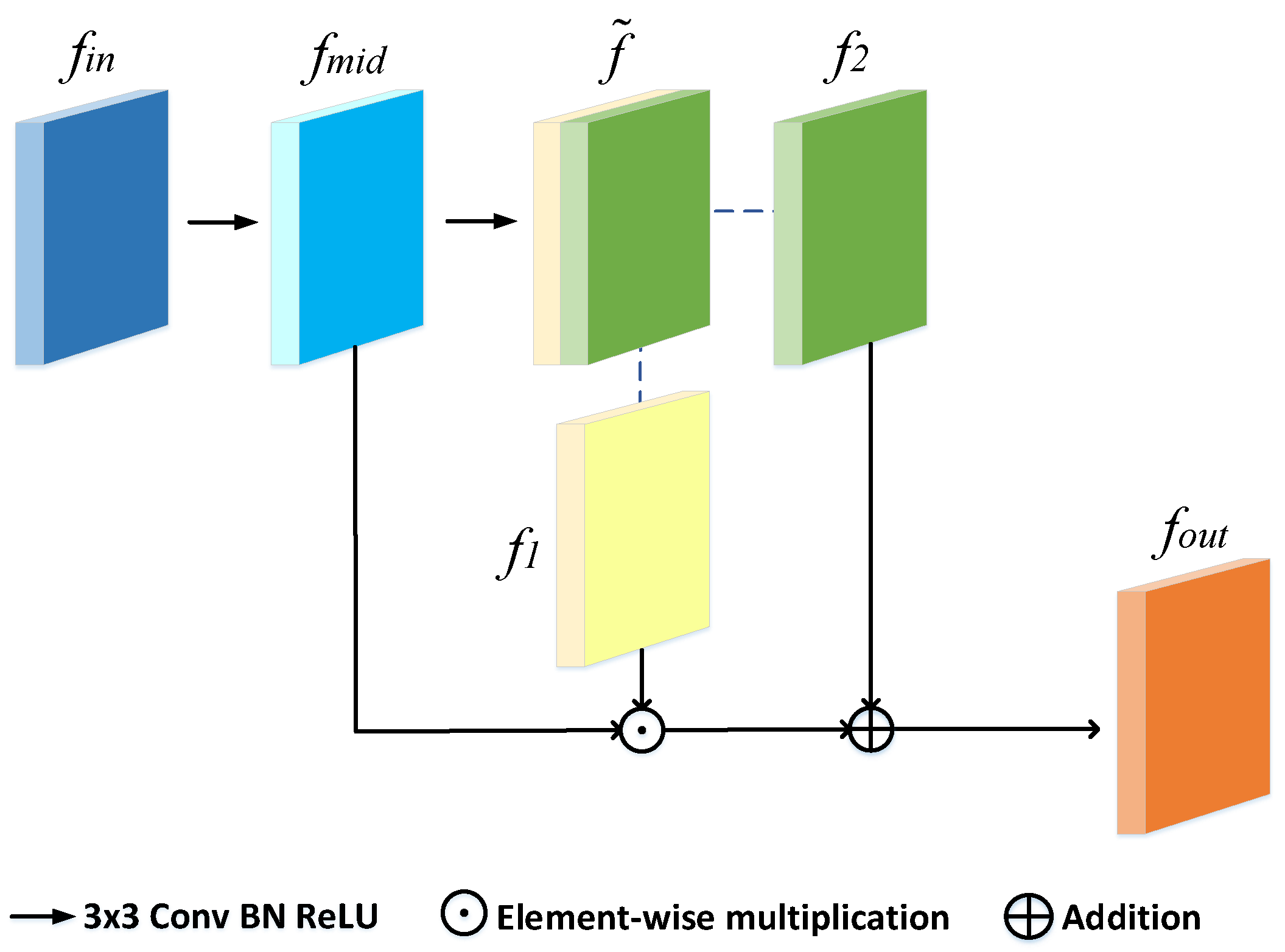
Figure 3.
Architecture of the intra-refinement module.
Figure 3.
Architecture of the intra-refinement module.
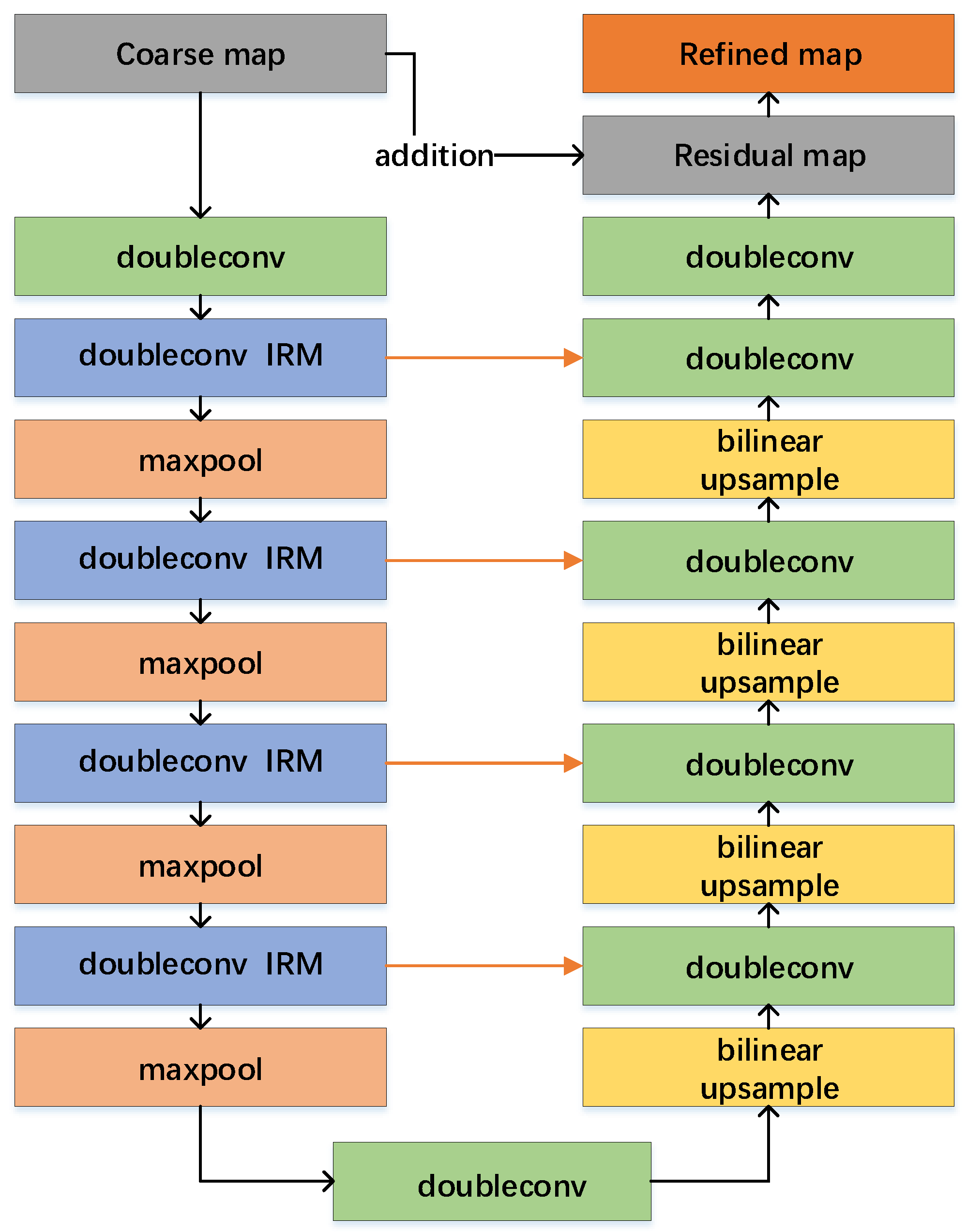
Figure 4.
Structure of the proposed residual refinement module. Doubleconv refers to two successive convolutions applied to extract features, followed by an intra-refinement module (IRM) to refine details.
Figure 4.
Structure of the proposed residual refinement module. Doubleconv refers to two successive convolutions applied to extract features, followed by an intra-refinement module (IRM) to refine details.
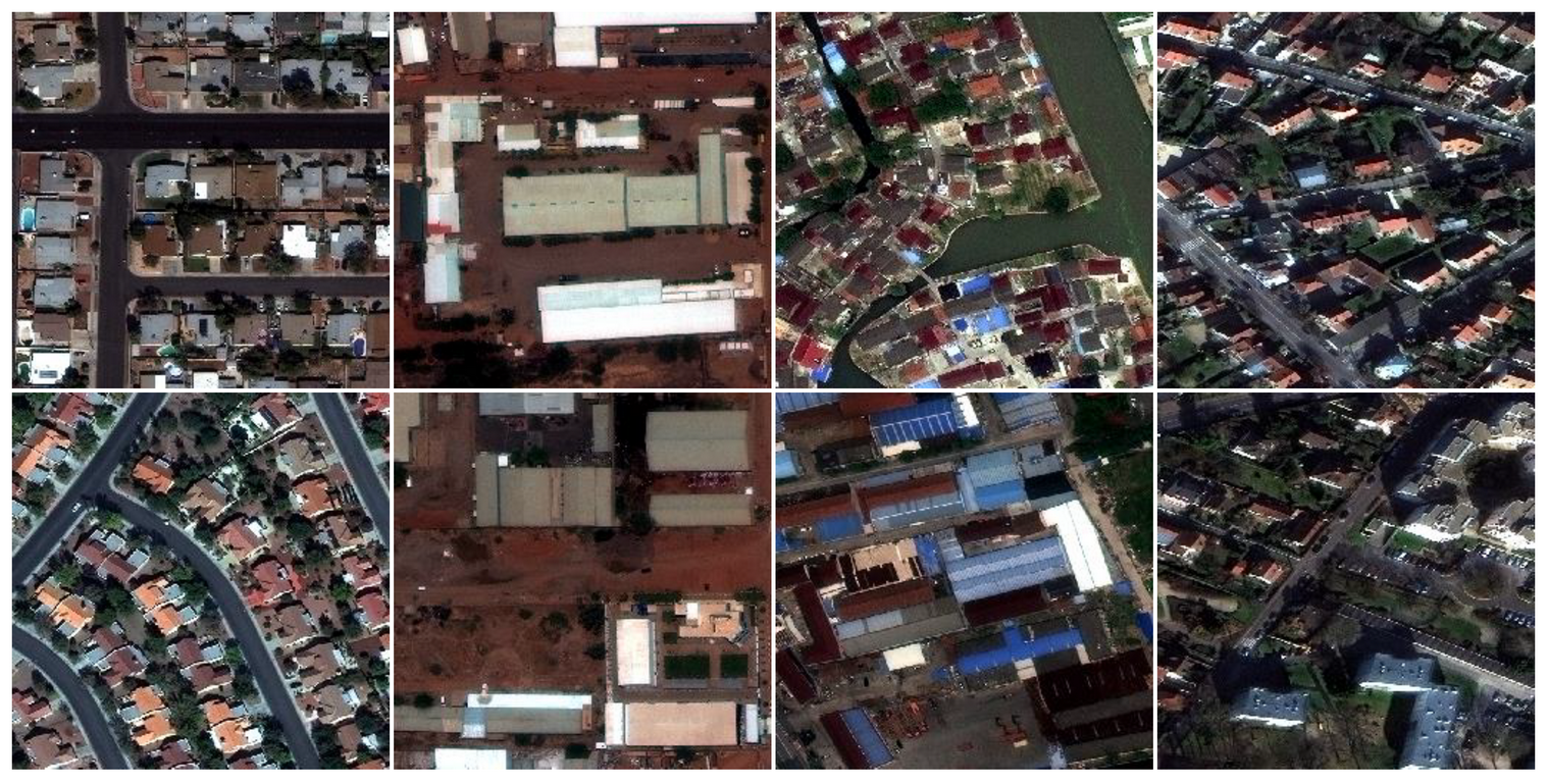
Figure 5.
Examples from four cities in the SpaceNet building dataset (from left to right): Las Vegas, Khartoum, Shanghai, and Paris.
Figure 5.
Examples from four cities in the SpaceNet building dataset (from left to right): Las Vegas, Khartoum, Shanghai, and Paris.
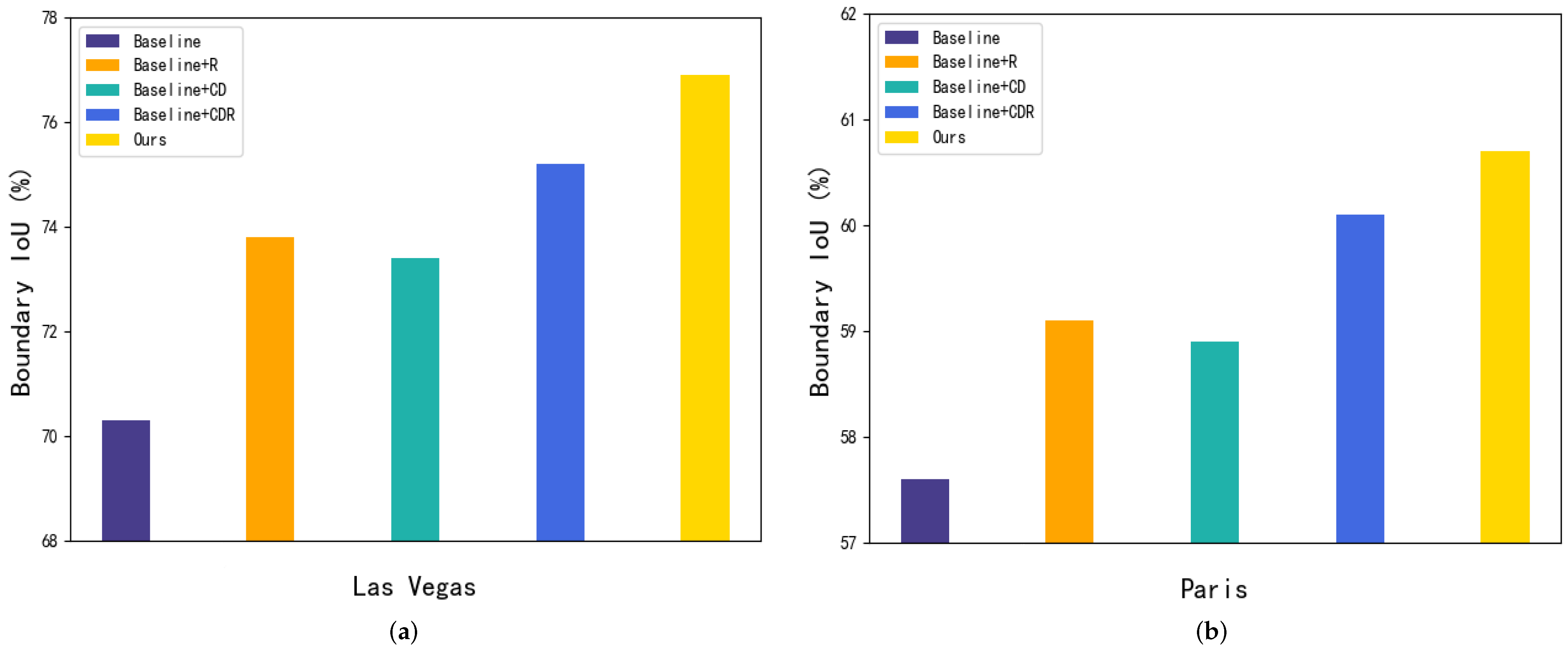
Figure 6.
Boundary IoU values for two cities after the addition of different modules: (a) the Las Vegas dataset and (b) the Paris dataset.
Figure 6.
Boundary IoU values for two cities after the addition of different modules: (a) the Las Vegas dataset and (b) the Paris dataset.
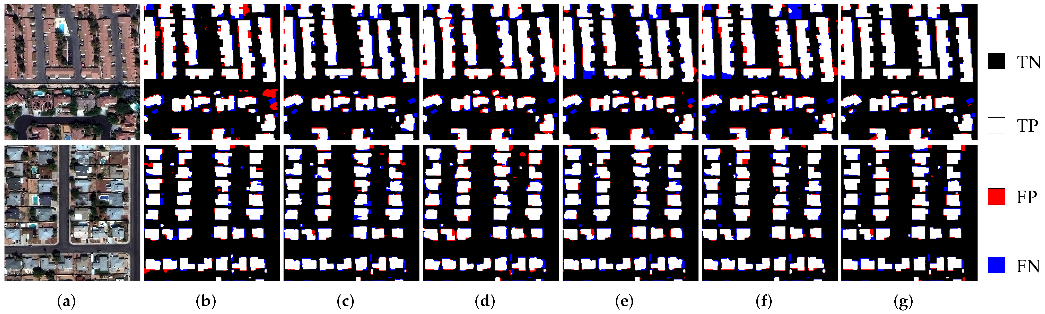
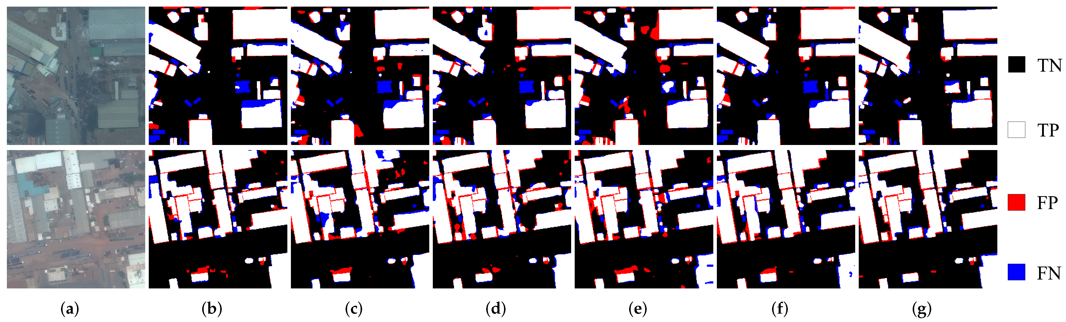
Figure 7.
Results of building segmentation in different regions of the Las Vegas dataset using six methods: (a) input image, (b) U-Net, (c) DeepLabV3+, (d) PSPNet, (e) UPerNet, (f) TransUNet, and (g) ours. Pixel-based true negatives, true positives, false positives, and false negatives are marked in black, white, red, and blue, respectively.
Figure 8.
Results of building segmentation in different regions of the Khartoum dataset using six methods: (a) input image, (b) U-Net, (c) DeepLabV3+, (d) PSPNet, (e) UPerNet, (f) TransUNet, and (g) ours. Pixel-based true negatives, true positives, false positives, and false negatives are marked in black, white, red, and blue, respectively.
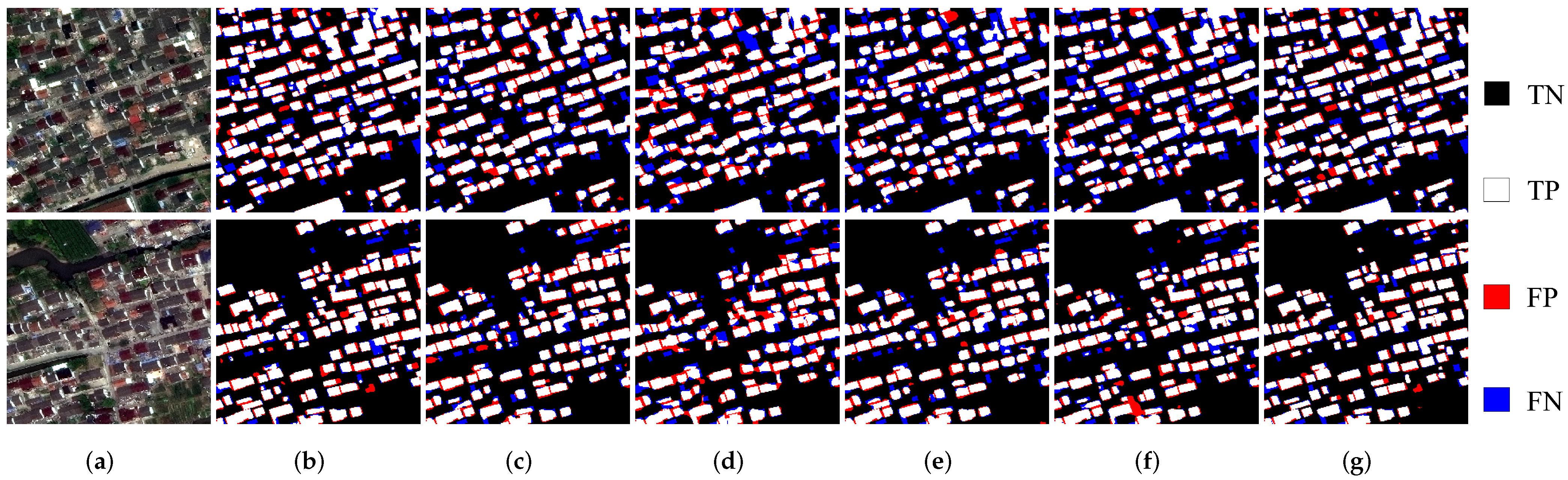
Figure 9.
Results of building segmentation in different regions of the Shanghai dataset using six methods: (a) input image, (b) U-Net, (c) DeepLabV3+, (d) PSPNet, (e) UPerNet, (f) TransUNet, and (g) ours. Pixel-based true negatives, true positives, false positives, and false negatives are marked in black, white, red, and blue, respectively.
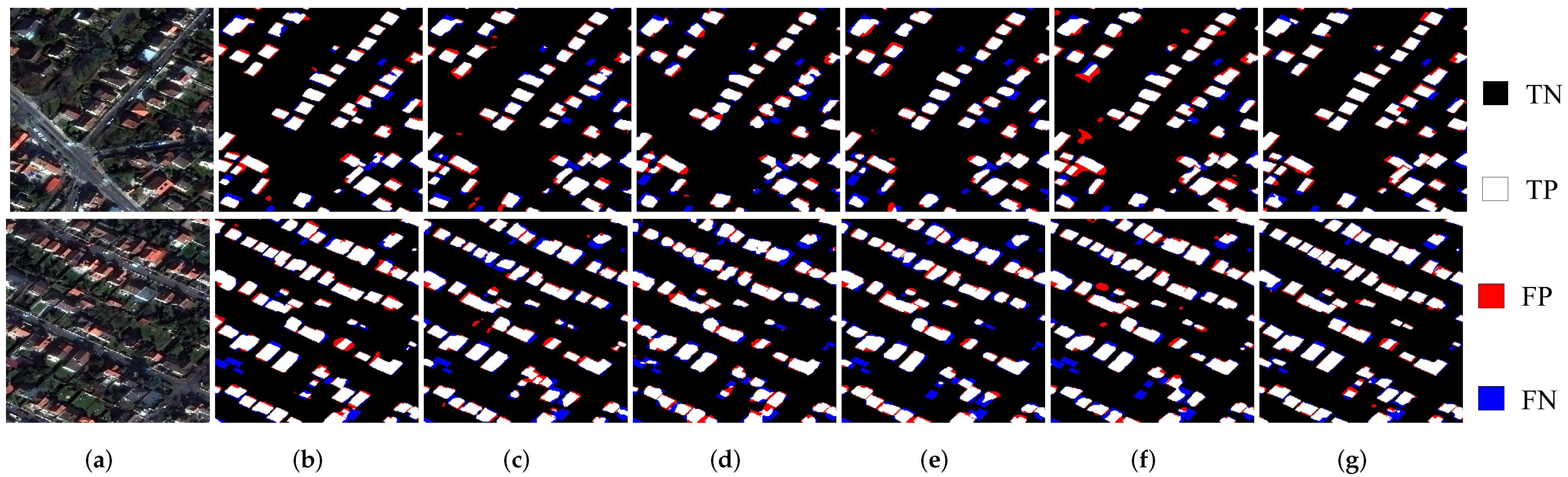
Figure 10.
Results of building segmentation in different regions of the Paris dataset using six methods: (a) input image, (b) U-Net, (c) DeepLabV3+, (d) PSPNet, (e) UPerNet, (f) TransUNet, and (g) ours. Pixel-based true negatives, true positives, false positives, and false negatives are marked in black, white, red, and blue, respectively.
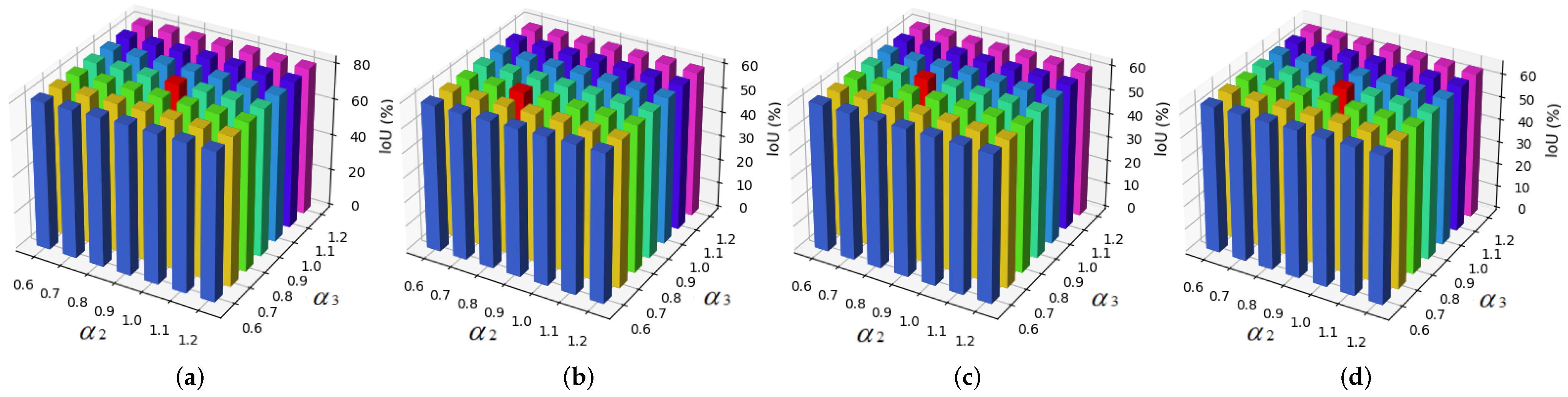
Figure 11.
Influences of different parameter values on the IoU values obtained for all four cities (each red pillar represents the best value). (a) IoU values on the Las Vegas dataset with different values of the parameters and . (b) IoU values on the Khartoum dataset with different values of the parameters and . (c) IoU values on the Shanghai dataset with different values of the parameters and . (d) IoU values on the Paris dataset with different values of the parameters and .
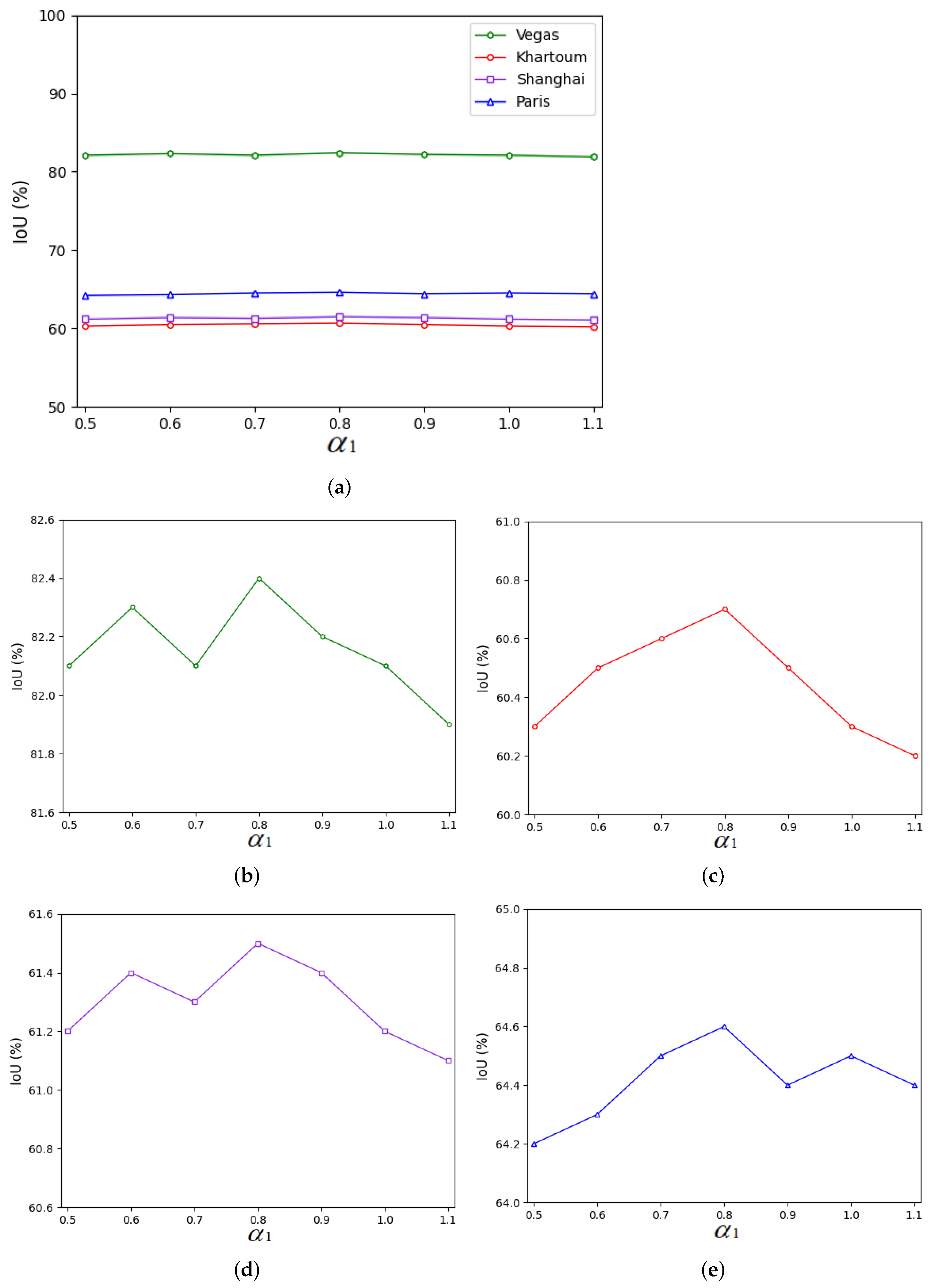
Figure 12.
Influences of different parameter values on the IoU values obtained for all four cities. (a) IoU values for all four cities with different values of the parameter . (b) IoU values on the Las Vegas dataset with different values of the parameter . (c) IoU values on the Khartoum dataset with different values of the parameter . (d) IoU values on the Shanghai dataset with different values of the parameter . (e) IOU values on the Paris dataset with the parameter .
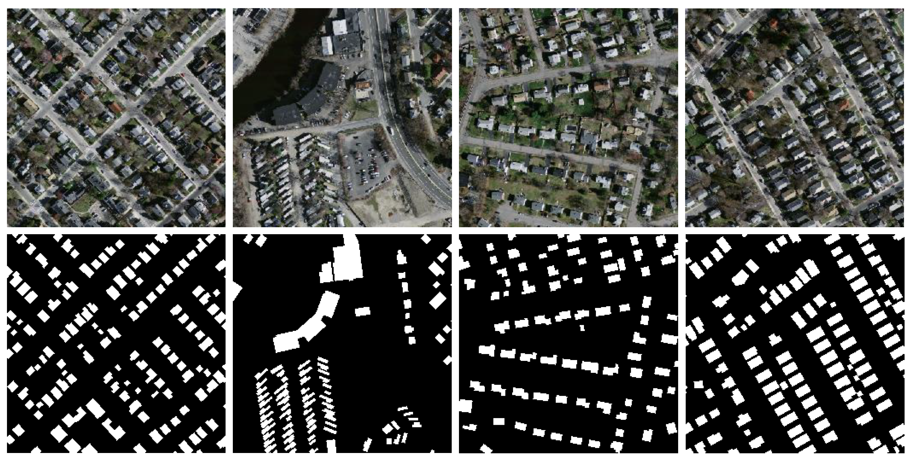
Figure 13.
Samples from the Massachusetts building dataset. RGB imagery and corresponding reference maps are displayed in the first and second rows, respectively.
Figure 13.
Samples from the Massachusetts building dataset. RGB imagery and corresponding reference maps are displayed in the first and second rows, respectively.
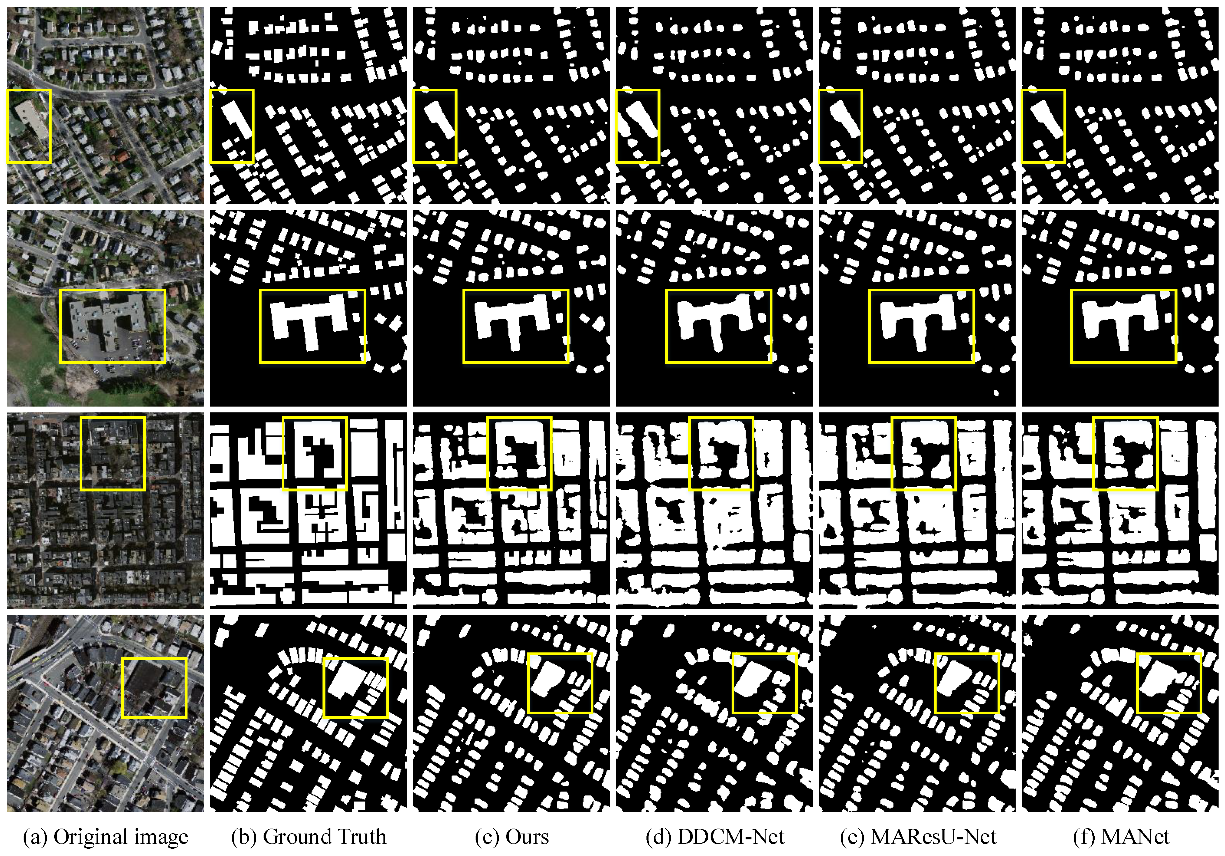
Figure 14.
Qualitative comparisons between our method and several recent studies on the Massachusetts building dataset. (a) Original image, (b) ground truth, (c) prediction map of ours, (d) prediction map of DDCM-Net, (e) prediction map of MAResU-Net, and (f) prediction map of MANet.
Figure 14.
Qualitative comparisons between our method and several recent studies on the Massachusetts building dataset. (a) Original image, (b) ground truth, (c) prediction map of ours, (d) prediction map of DDCM-Net, (e) prediction map of MAResU-Net, and (f) prediction map of MANet.
Table 1.
Numbers of images and building footprints across the areas of interest in SpaceNet.
Table 1.
Numbers of images and building footprints across the areas of interest in SpaceNet.
| City | Number of Images | Resolution (m) | Raster Area () |
|---|
| Las Vegas | 3851 | 0.3 | 216 |
| Khartoum | 1012 | 0.3 | 765 |
| Shanghai | 4582 | 0.3 | 1000 |
| Paris | 1148 | 0.3 | 1030 |
| Total | 10,593 | | 3011 |
Table 2.
Results of an ablation study of different modules obtained on the Las Vegas dataset. C, contour extraction; D, distance estimation; R, residual refinement module; I, intra-refinement module; M, multistage outputs.
Table 2.
Results of an ablation study of different modules obtained on the Las Vegas dataset. C, contour extraction; D, distance estimation; R, residual refinement module; I, intra-refinement module; M, multistage outputs.
| Method | OA (%) | Precision (%) | Recall (%) | F1-Score (%) | IoU (%) | Increase in IoU (%) |
|---|
| Baseline | 95.4 | 85.9 | 87.5 | 85.9 | 77.0 | - |
| Baseline + C | 95.7 | 87.3 | 87.9 | 86.9 | 78.3 | 1.3 |
| Baseline + CD | 96.0 | 88.3 | 88.4 | 88.0 | 79.7 | 2.7 |
| Baseline + CDR | 96.4 | 89.7 | 88.1 | 88.6 | 80.8 | 3.8 |
| Baseline + CDI | 96.3 | 89.4 | 88.4 | 88.5 | 80.6 | 3.6 |
| Baseline + CDM | 96.2 | 89.4 | 88.4 | 88.6 | 80.5 | 3.5 |
| Baseline + ALL | 96.6 | 91.2 | 88.8 | 89.6 | 82.4 | 5.4 |
Table 3.
Results of an ablation study of different modules obtained on the Paris dataset. C, contour extraction; D, distance estimation; R, residual refinement module; I, intra-refinement module; M, multistage outputs.
Table 3.
Results of an ablation study of different modules obtained on the Paris dataset. C, contour extraction; D, distance estimation; R, residual refinement module; I, intra-refinement module; M, multistage outputs.
| Method | OA (%) | Precision (%) | Recall (%) | F1-Score (%) | IoU (%) | Increase in IoU (%) |
|---|
| Baseline | 95.3 | 77.6 | 73.9 | 73.8 | 61.9 | - |
| Baseline + C | 95.5 | 77.5 | 72.7 | 74.0 | 62.4 | 0.5 |
| Baseline + CD | 95.6 | 76.5 | 73.4 | 74.3 | 62.7 | 0.8 |
| Baseline + CDR | 95.8 | 79.0 | 75.9 | 75.5 | 63.6 | 1.7 |
| Baseline + CDI | 95.7 | 79.1 | 73.2 | 74.1 | 63.2 | 1.3 |
| Baseline + CDM | 95.7 | 78.9 | 75.0 | 75.6 | 63.3 | 1.4 |
| Baseline + ALL | 95.9 | 78.9 | 74.9 | 75.8 | 64.6 | 2.7 |
Table 4.
Comparison of the building extraction results obtained by different methods on the Las Vegas test dataset.
Table 4.
Comparison of the building extraction results obtained by different methods on the Las Vegas test dataset.
| Method | OA (%) | Precision (%) | Recall (%) | F1-Score (%) | IoU (%) |
|---|
| U-Net | 95.4 | 85.6 | 87.5 | 85.9 | 77.0 |
| DeepLabV3+ | 95.8 | 89.3 | 85.9 | 87.2 | 78.5 |
| PSPNet | 95.5 | 87.5 | 87.3 | 88.7 | 78.1 |
| UPerNet | 95.7 | 89.2 | 86.1 | 87.2 | 78.6 |
| TransUNet | 95.6 | 87.8 | 86.1 | 86.3 | 77.4 |
| Ours | 96.6 | 91.2 | 88.8 | 89.6 | 82.4 |
Table 5.
Comparison of the building extraction results obtained by different methods on the Khartoum test dataset.
Table 5.
Comparison of the building extraction results obtained by different methods on the Khartoum test dataset.
| Method | OA (%) | Precision (%) | Recall (%) | F1-Score (%) | IoU (%) |
|---|
| U-Net | 92.7 | 77.3 | 71.5 | 71.5 | 58.3 |
| DeepLabV3+ | 91.7 | 71.7 | 66.9 | 67.2 | 53.2 |
| PSPNet | 92.5 | 72.3 | 69.8 | 69.5 | 56.3 |
| UPerNet | 91.7 | 71.4 | 68.7 | 67.1 | 53.1 |
| TransUNet | 92.1 | 71.8 | 72.6 | 70.1 | 56.4 |
| Ours | 92.8 | 76.7 | 73.8 | 73.6 | 60.7 |
Table 6.
Comparison of the building extraction results obtained by different methods on the Shanghai test dataset.
Table 6.
Comparison of the building extraction results obtained by different methods on the Shanghai test dataset.
| Method | OA (%) | Precision (%) | Recall (%) | F1-Score (%) | IoU (%) |
|---|
| U-Net | 94.5 | 75.8 | 71.7 | 72.0 | 60.2 |
| DeepLabV3+ | 93.7 | 73.9 | 67.5 | 69.1 | 56.8 |
| PSPNet | 94.4 | 75.6 | 70.4 | 71.4 | 59.6 |
| UPerNet | 93.9 | 75.2 | 65.7 | 68.0 | 55.9 |
| TransUNet | 93.7 | 71.8 | 67.4 | 67.6 | 55.5 |
| Ours | 94.6 | 77.6 | 71.2 | 73.1 | 61.5 |
Table 7.
Comparison of the building extraction results obtained by different methods on the Paris test dataset.
Table 7.
Comparison of the building extraction results obtained by different methods on the Paris test dataset.
| Method | OA (%) | Precision (%) | Recall (%) | F1-Score (%) | IoU (%) |
|---|
| U-Net | 95.3 | 77.6 | 73.9 | 73.8 | 61.9 |
| DeepLabV3+ | 94.7 | 74.1 | 70.3 | 70.1 | 57.2 |
| PSPNet | 95.3 | 77.3 | 72.1 | 73.6 | 61.1 |
| UPerNet | 94.6 | 75.8 | 67.2 | 69.9 | 56.7 |
| TransUNet | 94.5 | 69.0 | 74.7 | 70.9 | 57.8 |
| Ours | 95.9 | 78.9 | 74.9 | 75.8 | 64.6 |
Table 8.
Comparison of the building extraction results obtained by the proposed method and recent methods on the Massachusetts building dataset.
Table 8.
Comparison of the building extraction results obtained by the proposed method and recent methods on the Massachusetts building dataset.
| Method | OA (%) | Precision (%) | Recall (%) | F1-Score (%) | IoU (%) |
|---|
| Ours | 94.11 | 88.20 | 81.99 | 84.98 | 73.89 |
| DDCM-Net [50] | 93.30 | 86.19 | 79.78 | 82.86 | 70.74 |
| MAResU-Net [51] | 93.49 | 85.46 | 81.87 | 83.63 | 71.86 |
| MANet [52] | 93.69 | 87.32 | 80.64 | 83.85 | 72.19 |


