Abstract
Time series of the Gravity Recovery and Climate Experiment (GRACE) satellite mission have been successfully used to reveal changes in terrestrial water storage (TWS) in many parts of the world. This has been hindered in the interior of the Tibetan Plateau since the derived TWS changes there are very sensitive to the selections of different available GRACE solutions, and filters to remove north-south-oriented (N-S) stripe features in the observations. This has resulted in controversial distributions of the TWS changes in previous studies. In this paper, we produce aggregated hydrology signals (AHS) of TWS changes from 2003 to 2009 in the Tibetan Plateau and test a large set of GRACE solution-filter combinations and mascon models to identify the best combination or mascon model whose filtered results match our AHS. We find that the application of a destriping filter is indispensable to remove correlated errors shown as N-S stripes. Three best-performing destriping filters are identified and, combined with two best-performing solutions, they represent the most reliable solution-filter combinations for determination of weak terrestrial water storage changes in the interior of the Tibetan Plateau from GRACE. In turn, more than 100 other tested solution-filter combinations and mascon solutions lead to very different distributions of the TWS changes inside and outside the plateau that partly disagree largely with the AHS. This is mainly attributed to less effective suppression of N-S stripe noises. Our results also show that the most effective destriping is performed within a maximum degree and order of 60 for GRACE spherical harmonic solutions. The results inside the plateau show one single anomaly in the TWS trend when additional smoothing with a 340-km-radius Gaussian filter is applied. We suggest using our identified best solution-filter combinations for the determination of TWS changes in the Tibetan Plateau and adjacent areas during the whole GRACE operation time span from 2002 to 2017 as well as the succeeding GRACE-FO mission.
1. Introduction
The Tibetan Plateau (TP) (25°~40°N and 75°~105°E) is both the highest and the largest plateau in the world. Since it is regarded as ‘the water tower of Asia’ and is very sensitive to global change, it is of major importance to understand the terrestrial water storage (TWS) changes in the plateau, not only for the utilization of water resources in the plateau and surrounding Asian countries but also for global change studies.
Terrestrial in situ hydrology observations to determine TWS changes have rarely been made due to the harsh weather conditions and the challenging geography in the plateau. Hence, time-variable gravity measurements of the Gravity Recovery and Climate Experiment (GRACE) twin-satellite mission since 2002 were warmly welcomed as they were seen as bright prospect in monitoring the regional TWS changes there (e.g., [1,2]).
Two types of time series of GRACE data products are provided which can be used for the estimation of TWS changes, (1) spherical harmonic (SH) gravity solutions consisting of monthly Stokes coefficients provided by different institutions, and (2) mass concentration (mascon) models, also provided by different institutions, which directly give the TWS changes in equivalent water thickness (EWT) on mascon grids.
When the TWS changes are derived based on a GRACE SH gravity solution, the precise determination of TWS changes is hampered on one hand by measurement noises, which increase with the harmonic degree, and on the other hand due to the prominent north-south-oriented (N-S) stripe effects from the orbital configuration of the twin satellites. It is thus indispensable to apply adequate post-processing with a destriping filter (e.g., the filter proposed by Swenson and Wahr [3]) and a smoothing filter (e.g., Gaussian filter proposed by Jekeli [4]), successively. Kusche et al. [5] proposed a non-isotropic filtering approach which can conduct destriping and smooth filtering simultaneously. In a mascon model, the stripe errors and measurement errors are effectively suppressed according to the developers and thus the users are advised to avoid any additional empirical destriping or smoothing (e.g., [6,7]).
While GRACE data products have been successfully used to derive TWS changes in many parts of the world (e.g., [8,9,10,11]), clear identification of TWS changes in the TP from GRACE is challenging. The magnitudes of potential TWS anomalies are small and in the order of about 15 mm/yr [2]. These are surrounded by much larger TWS anomalies due mainly to glacier melting in the mountains and groundwater extraction from Northwest India to the Bengal Basin in the order of 25-50 mm/yr [2]. Previous studies providing TWS changes based on GRACE products from different agencies and using various data-processing strategies thus show significant discrepancies over the TP (e.g., [12,13]). A dozen publications show TWS changes in the plateau interior with very different features, which includes the number, position, and magnitude of TWS anomalies (see Table 1). This may be partially attributed to different time periods or different averaging radius values of the Gaussian filters. However, their effects are far less than those from the selection of the GRACE data type and solution(s), and especially the chosen destriping filter(s). As Table 1 shows, different GRACE solutions using various data-processing filters, or even the same solution using different data-processing, lead to very controversial patterns of the GRACE-derived TWS changes in the interior of the TP: The number of mass increase anomalies varies between one and five, and they are located in the east or west by north or south or in the center of the plateau.

Table 1.
Overview of terrestrial water storage trend rates inside the Tibetan Plateau from previous works.
Erkan et al. [14], for example, used the CSR SH solutions [24] together with the destriping method by Duan et al. [22] to find two signal anomalies in the plateau, a smaller one in the west and a larger one in the east. Jiao et al. [16] instead used the level-3 data products derived from JPL SH solutions in combination with the destriping method by Swenson and Wahr [3] and found only one anomaly in the eastern plateau. If no destriping filters are applied, the number of the derived TWS anomalies usually increases [12,18,20]. We also noticed, solely by visual inspection, large discrepancies between the CSR_M, JPL_M and GSFC_M mascon model results in Jing et al. [13] and Loomis et al. [21].
We can summarize at least two reasons for the different previous results and the challenge to extract TWS changes in the TP: (1) Measurement noises, orbit errors and different strategies for producing GRACE solutions condition the fact that solutions from different agencies vary conspicuously; (2) Compared to other places, the hydrological conditions and their changes in the TP and adjacent areas are so special that the magnitudes of the TWS changes inside the plateau are small, and so can be easily falsified by the superimposed interference signals from nearby strong TWS signals—especially when using destriping and spatial smoothing filters for SH solutions. Hence, an adequate postprocessing of GRACE data must be tailored for clear determination of TWS changes in the TP.
The controversial TWS changes summarized in Table 1 may confuse readers and make them wonder which TWS change results are reliable in the TP. Based on currently existing GRACE solutions (including SH solutions and mascon models) and various destriping filters (e.g., destriping methods by Swenson and Wahr [3] and Duan et al. [22]), our aim is to identify the best GRACE solution-filter combinations and to obtain most reliable and reasonable TWS changes for the TP. This would close discussions on this controversial subject and provide guidelines for future studies on TWS changes in the TP and adjacent areas.
The criterion for choosing a certain solution-filter combination should be given by independent data serving as some kind of ‘ground truth’. Considering the harsh weather conditions, challenging geography and thus rare in situ measurement of TWS changes in the TP, an aggregated TWS hydrology signal of the few available GRACE-independent observations of contributing signals is suggested herein. GRACE-derived TWS changes in the TP consist of changes in various water storage components, including soil moisture, glacier mass, snow water storage, lake water, permafrost and groundwater [2]. These contributions can be obtained from previous studies based on multiple altimetric missions, optical satellite imagery, hydrological models (e.g., GLDAS [25]) and changes in permafrost degradation calculated from an Active-Layer Depth (ALD) model [14,26]. The results from previous works are obtained through rigorous methods and techniques, and they usually have relatively small errors [27,28,29,30] or have been proven a good applicability in the TP [31,32]. Given the small errors, and that any additional water storage components in the TP have not been identified yet, the aggregated hydrology signals (AHS) of these different results should represent the currently best available ‘ground truth’ criterion for GRACE-derived TWS changes with relatively low spatial resolution (300–400 km). Moreover, many previous studies that also used a combination of GRACE and satellite altimetry and hydrological models for water storage change investigations got very good results [2,12,16,33,34,35].
We test about 130 combinations of GRACE solutions and destriping filters and some mascon models until the derived TWS changes agree with the AHS of the same period. We note that all these solutions, destriping methods and models are known and well established, thus we do not aim to introduce a new filtering approach or model.
In the next section, the used GRACE solutions and destriping filters are briefly introduced. In Section 3, the calculation of the GRACE-derived TWS changes and the AHS are shown, followed by the presentation and discussion of the results in Section 4. Finally, we summarize our findings in Section 5.
2. GRACE Solutions and Destriping Filters
2.1. GRACE Solutions
We apply fifteen different newly released monthly GRACE solutions, i.e., twelve SH solutions and three mascon models. The time span covers the period from April 2002 to June 2017. Twelve newly updated SH solutions are ITSG [36], CSR [24], COST-G [37], JPL [38], GFZ [39], Tongji [40], WHU [41], HUST [42], GRGS [43], IGG [44], AIUB [45] and XISM [46]. The different SH solutions are provided with Stokes coefficients of different maximum degrees such as 60, 90 and 96. We made tests to ensure the proper maximum degree since the Stokes coefficients become noisier with higher degrees, which needs an effective destriping filter to depress the N-S stripe noises. The glacial isostatic adjustment (GIA) effects are removed from the monthly Stokes coefficients according to the GIA model ICE-6G_C(VM5a) [47].
The three global equal area mascon models are CSR_M [6], JPL_M [48] and GSFC_M [49]. CSR_M is derived from GRACE information only [6], while JPL_M contains next to GRACE information and a-priori information of mass variations as constraints, which are from land, ocean, ice, inland sea, large inland lake, earthquake and glacial isostatic adjustment [48]. GSFC_M uses the signal auto-covariance matrix as a regularization constraint, and is constructed by spatio-temporal constraint equations [49,50]. To be applicable for comparison in this study, we decompose the mascon grid EWT data into SH Stokes coefficients from degree 1 to 90.
Considering the absence of degree-1 coefficients and inaccuracy of C20 and C30 coefficients for SH solutions, we complement GRACE SH solutions with newly released C10, C11 and S11 coefficients [51], and replace the native GRACE C20 and C30 coefficients with the latest SLR-derived version [52]. We note that the C30 coefficients were replaced when the time series passed March 2012, where the SLR-derived C30 starts in the data set according to Loomis et al. [52].
2.2. Destriping Filters
The monthly Stokes coefficients of each GRACE SH solution are destriped with three frequently used destriping methods proposed by Duan et al. [22], Swenson and Wahr [3] and Chambers [23], respectively. For each of the three methods, a polynomial of selected degree x is used in a window of width w, fitted to all the coefficients of the same parity in degrees ≥y for a certain order (≥y), and the coefficients used in fitting are subtracted by the fitting values. In this way, the correlated errors which manifest as N-S stripes can be reduced in the coefficients within the window. Thus, a series of the destriping filters named ‘Duan PxMy’, ‘S&W PxMy’ and ‘Cham PxMy’ in this study can be devised and used for x = [ 2, 3, 4] and y = 8. These values were found to perform well in earlier studies [53]. The filters ‘Duan P4M10’, ‘Duan P4M15’, ‘S&W P3M10’ and ‘S&W P3M15’ are additionally considered in order to observe the effects of different y values.
Destriping filters ‘Duan PxMy’ and ‘S&W PxMy’ use moving filtering windows. According to Duan et al. [22], the width w for ‘Duan PxMy’ filtering is calculated using Equation (1), dependent on the degree l and order m of the coefficients to be filtered and the parameters () taking empirical values (0.1, 3, 30, 15),
However, for ‘S&W PxMy’ filtering, w is calculated using Equation (2), dependent on the order m of the coefficients, and the parameters taking the values (30, 10),
For ’Cham PxMy’ filtering, the windows include all the coefficients of the same parity in degrees from y to 90 (or 96) for a certain order (also ≥y).
Piretzidis et al. [54] developed a method of identifying and selectively destriping SH coefficients with correlated errors by utilizing the capabilities of machine learning algorithms (MLAs), which can be used to calculate monthly changes in TWS [54], and this destriping method is marked by ‘MLAs’ here.
The monthly Stokes coefficients can also be destriped and smoothed simultaneously for each GRACE gravity SH solution with the non-isotropic filtering approach proposed by Kusche et al. [5]. We choose the filter DDK8 for four gravity SH solutions (ITSG/CSR/JPL/GFZ) and the much stronger filters DDK2 for the preferred ITSG model to show their performances, respectively. According to Kusche et al. [5], the filtering characteristics of the DDK2 filter are approximately equivalent to a Gaussian filter with an averaging radius of 340 km.
3. Calculation of GRACE-Derived TWS Change and Aggregated Hydrology Signal
3.1. GRACE-Derived TWS Change
According to Wahr et al. [55], the monthly TWS changes (in EWT) can be derived at an any grid site with co-latitude and longitude on grids covering our study area with
in which and are the changes in Stokes coefficients from GRACE gravity SH solutions or decomposed from three mascon models, is the lth degree and mth order normalized associated Legendre polynomial, is the degree l elastic load Love number of the Preliminary Reference Earth Model for potential perturbation [56], is the average density of the earth, is the water density and a is the radius of the Earth. The derived TWS changes are expressed as EWT converted to the unit of millimeter.
In order to analyze the features of the monthly TWS changes in the TP and adjacent areas, the trend rate, annual change at each grid point, together with a semi-annual and a 161 days aliasing variation (from the S2 semidiurnal solar tide), are simultaneously estimated using a least-square linear regression.
3.2. Aggregated Hydrology Signal
The AHS (denoted by trend rates of EWT changes) from 2003 to 2009 (and 2016) represent the total TWS changes from soil moisture (SM), glacier ice (ICE), lake water (LAKE) and permafrost (PM) in the TP and adjacent areas. Groundwater storage (GWS) contributions have not yet been assessed independent of GRACE data in this region and thus are not included in the AHS. Signal changes caused by snow and ICE on glaciers were coupled following Gardner et al. [28], which we marked as ICE, while internal testing yielded that snow out of glaciers has a negligible impact. Hence, snow is not added in the AHS. Further, we assume that the AHS represent the basic features of realistic TWS changes inside the plateau except for the eastern plateau where the increase in GWS signals is too strong to be neglected as a component of TWS changes [2]. Hence, the eastern plateau is omitted when determining the best GRACE solution-filter combination.
For comparisons of the GRACE-derived TWS changes with the AHS, the contribution of each hydrology component is also derived with Equation (3) in Xiang et al. [2], summed till degree 60 (and 90, for evaluating the reliability of the simulated TWS changes derived from different maximum d/o). However, when deriving the contributions, mass change for the hydrology component K (= SM, ICE, LAKE or PM) can be represented as , and thus, the changes in spherical harmonic coefficients , are given by decomposition of corresponding grid data designed referring to xiang et al. [2] in our surveyed area () using
with . The integrations of Equation (4) can be easily solved by summing the contributions of all the grids for SM, ICE, LAKE and PM, respectively.
The hydrology components can be given by trend rates of EWT changes from 2003 to 2009. The grid SM data are from three different land surface models: Noah, Variable Infiltration Capacity (VIC) and Catchment Land Surface Model (CLSM) of GLDAS-2.1 which is forced with a combination of model and observation data from 2000 to present [25]. The LAKE data for 219 lakes are combined from Zhang et al. [27] and Farinotti et al. [29], and the ICE data are taken from Gardner et al. [28]—all are based on the analysis of ICESat-1 data. Since grid PM data are not available during our surveyed period, we follow Xiang et al. [2] and use trends of active-layer depth in the plateau from 1980 to 2001 by Oelke and Zhang [26] and Erkan et al. [14]. For comparison purposes over a longer period, the hydrology components are also given by trend rates of EWT changes from 2002 to 2016, using the grid SM data from Noah, VIC and CLSM of GLDAS, PM data based on Xiang et al. [2], LAKE data for 61 lakes derived from Li et al. [57] and LEGOS HYDROWEB [30] based on multi-source remote sensing, and the ICE data from Brun et al. [58] using time series of digital elevation models derived from ASTER optical satellite stereo-imagery.
4. Results and Discussion
4.1. Selection of the Solution-Filter Combination
4.1.1. Correlation Check
We calculated trends in the TWS changes from 2003 to 2009 in the TP and adjacent areas, based on the 130 solution-filter combinations outlined above and three mascon solutions. The best solution-filter combination(s) is determined by applying Pearson’s correlation coefficients (PCC-values), Root Mean Square Errors (RMSE-values) and Index Of Agreement values (IOA-values) between the GRACE-derived trends of TWS changes and the AHS during the same period in a selected region of the plateau interior (as shown in Table 2 and Table A1), which are intended to show their pattern and magnitude agreements of observed and aggregated models. PCC-values, RMSE-values and IOA-values are calculated using Equations (A1)–(A3) respectively.
Table 2.
PCC-, RMSE- and IOA-values between the GRACE-derived TWS trends of selected GRACE solution centers (as in Figure 1a–l and Figure 2a–h) and the aggregated hydrology signals in our chosen comparison area inside the plateau (Figure 3f). Additional results for 7 more solution centers can be found in Table A1. The best-performing filters are separated by two dashed lines.
In order to verify the effectiveness of the selected best solution-filter combination(s) over a longer period, we also obtained PCC-, RMSE- and NSE-values between GRACE-derived trends of TWS changes based on five selected solution-filter combinations and AHS from 2002 to 2016 (Figure A6). Similarly, for exploring the effects of higher d/o Stokes coefficients (i.e., from 61 to 90) on the inversed TWS changes, we repeated the calculations mentioned above, but with Stokes coefficients truncated at maximum d/o 90 (Figure A8, Figure A9 and Figure A10).
Figure 1 and Figure 2 and Table 2 and Table A1 show that the results can vary drastically. The ITSG and CSR solution together with ‘Duan P4M8’, ‘S&W P2M8’ and ‘S&W P3M8’ result as best combinations for their analogous outstanding performance with PPC-values larger than 0.66, RMSE-values smaller than 5.95 and IOA-values larger than 0.76, except for CSR together with S&W P2M8. We show only ITSG results since results for other SH solutions are quite similar to those of the ITSG solution (Figure 1), and for similar reasons, we only show results derived using the ‘S&W P3M8’ filter (Figure 2). The variability of the results in the two figures will be discussed in Section 4.1.2 and Section 4.1.3.
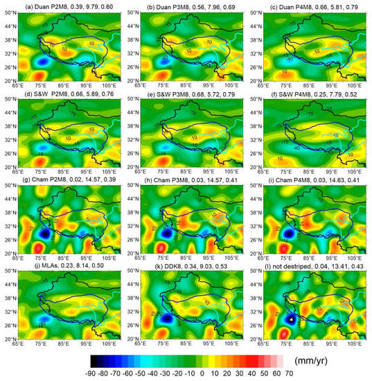
Figure 1.
Trend rates of terrestrial water storage (TWS) changes from 2003 to 2009 in the Tibetan Plateau and adjacent areas derived from the ITSG GRACE solution truncated at d/o 60 with different destriping filters (a–k) (see Section 2.2 for definition) and without destriping (l), compared with the aggregated hydrology signals (Figure 3f). Numbers on top are PCC-values (left), RMSE-values (Middle) and IOA-values (right) between the GRACE TWS signals (a–l) and the aggregated hydrology signals in the plateau interior delimited by red lines (see Figure 3f). The black lines indicate the national borders of China, the blue lines delimit the range of the Tibetan Plateau, and the cyan lines are the Yangtze and Yellow rivers.
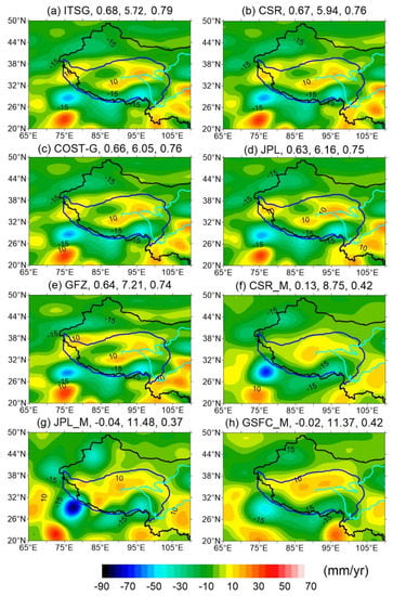
Figure 2.
Same as Figure 1 but for different GRACE solutions using destriping filter ‘S&W P3M8’ (a–e) and synthesized results (f–h) with decomposed Stokes coefficients d/o 1-60 from three mascon models. GRACE solutions are explained in Section 2.1.
The AHS from 2003 to 2009 in the TP and adjacent areas are shown in Figure 3f. Large negative signals are found in the Tien Shan (with magnitudes of ~35.0 mm/yr), the western/central/eastern Himalayas (~26.0 mm/yr, ~28.0 mm/yr, ~35.0 mm/yr) and the mountains southeast of the plateau (~28.0 mm/yr) mainly due to considerable ice melting. However, smaller signals consisting of three positive anomalies and one negative anomaly are found in the plateau interior. The western positive anomaly (~14.0 mm/yr) is a result of increased ice and soil moisture accumulation in the West Kunlun Mountains and slightly increasing lake water according to Figure 3a–c. The northeastern positive anomaly (~9.0 mm/yr) results from a combination of increased soil moisture and lake water mainly in Qinghai Lake. The positive anomaly (~11.5 mm/yr) to the south of the central TP is a comprehensive effect of lake water increase (~15.0 mm/yr) in the center of the plateau, the decrease in soil moisture to the southwest of the plateau, as well as a relatively small positive signal caused by spherical harmonic truncation from ICE. The prominent negative anomaly (~13.0 mm/yr) is mainly due to glacial melting in east Kunlun and the inner plateau [28] and permafrost degradation in the plateau, as well as the effects from soil moisture decreasing there.
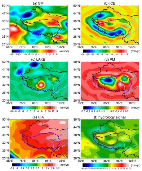
Figure 3.
SH trend rates of TWS components, GIA and the aggregated hydrology signals from 2003 to 2009, synthesized with SH coefficients truncated at d/o 60. Data sources: (a) monthly GLDAS (NOAH/VIC/CLSM) [25], (b) ICESat-1 based glacier measurements [28], (c) ICESat-1 lake measurements and LEGOS Hydroweb (e.g., [27,29,30]), (d) one ALD model [14,26], (e) ICE-6G_C(VM5a) model [47] and (f) aggregated hydrology signals representing the sum of four hydrological components (a–d).
In an area of the plateau interior delimited by red lines in Figure 3f, the AHS can be used as a ground truth for selection of the favorable GRACE solution(s) and destriping filter(s) for the TP interior. This marked target area is distant from the surrounding (glaciated) mountains where strong hydrology signals may impact the GRACE-derived TWS changes inside the plateau through signal leakage. It also excludes the eastern part of the plateau where possible obvious GWS changes [2] could not be modeled.
In Table 2 and Table A1, the PCC-, RMSE- and IOA-values are given for all tested solution-filter combinations and mascon models. The larger PCC- and IOA-values (in general PCC-values > 0.60, IOA-values > 0.70), and the smaller RMSE-values (in general RMSE-values < 6.40, except for GFZ) are obtained for combinations of destriping filters ‘Duan P4M8’, ‘S&W P2M8’ and ‘S&W P3M8’ with five GRACE SH solutions listed in Table 2. The agreement of GRACE-derived TWS trend rates with the AHS in the plateau interior is supported by visual comparison in Figure 1c–e and Figure 2a–e with Figure 3f. All other destriping filters generally result in much smaller PCC- and IOA-values, and much larger RMSE-values, implying that they are probably less effective, which we will verify in Section 4.3. All three mascon models also lead to much smaller PCC- and IOA-values, and much larger RMSE-values (in Figure 2f–h), showing that they disagree extremely with the AHS. Possible causes for this are discussed in Section 4.4.
4.1.2. Filter Dependence of the GRACE-Derived TWS Trends
In Figure 1a–k, the results of the GRACE-derived TWS trends from the best performing ITSG solution show obvious N-S variability depending on the selected destriping method, and E-W variability depending on the selected filter parameter (polynomial degree x = {2,3,4}). The results can be compared with those with original N-S stripes for the not-destriped case (Figure 1l). Particularly, they are compared with the AHS in the selected region inside the plateau (Figure 3f) to check their pattern and magnitude agreement. No obvious N-S stripes and better pattern and magnitude agreement (e.g., PCC-values 0.66, RMSE-values 5.95 and IOA-values 0.76) would imply a reasonable selection of the destriping filter(s).
Figure 1a–f show results applying the destriping methods by Duan et al. [22] and Swenson and Wahr [3], respectively. Both apply moving windows of variable width. For the filters with x = 2, 3 and 4, the N-S stripes are effectively depressed in the GRACE-derived trends both inside and outside the plateau. However, better pattern and magnitude agreement of the results with the AHS (Figure 3f) is found only for ‘Duan P4M8’, ‘S&W P2M8’ and ‘S&W P3M8’, with larger PCC-values of 0.66, 0.66 and 0.68, and IOA-values of 0.79, 0.76 and 0.79, as well as smaller RMSE-values of 5.81, 5.89 and 5.72, respectively.
We compare the destriping method of Chambers [23] with a non-moving window but with variable widths depending on the start order y (Figure 1g–i) with the non-destriped case (Figure 1l). For filters with x = 2, 3 and 4, visible N-S stripes remain inside and outside the plateau. As we also find much smaller PCC- and IOA-values, and much larger RMSE-values than those mentioned above, we think that these destriping filters are less effective. In Figure 1k, the results of the DDK8 filter also show some N-S stripes especially outside the plateau, and have a smaller PCC-value of 0.34, a smaller IOA-value of 0.53, and a larger RMSE-value of 9.03. This weaker filtering was already mentioned by Kusche et al. [5]. In Figure 1j, although there are no obvious N-S stripes inside the plateau, PCC- and IOA-value are small, the RMSE-value is so large that they also imply a less effective destriping filter.
We have further tested four destriping filters ‘Duan P4M10’, ‘Duan P4M15’, ‘S&W P3M10’ and ‘S&W P3M15’ having higher start orders than our previous tests. These results (Figure A1) are very similar in the pattern and the amplitude to those for the filters ‘Duan P4M8’ and ‘S&W P3M8’. However, the PCC- and IOA-values are smaller and RMSE-values are larger than those for ‘Duan P4M8’ and ‘S&W P3M8’, respectively, and become rapidly smaller (for PCC- and IOA-values) and larger (for RMSE-values) as the start orders become larger from 8 to 15, thus we suggest that the start order y = 8 is adequate for the tested destriping filters, which was also suggested by Swenson and Wahr [3] when they introduced the filter.
4.1.3. Solution Dependence of the GRACE-Derived TWS Trends
Figure 2 shows TWS trends from the five GRACE SH solutions ITSG, CSR, COST-G, JPL and GFZ filtered with one of the best performing filters, ‘S&W P3M8’, and from the three mascon models CSR_M, JPL_M and GSFC_M. The results can be compared with the AHS (Figure 3f) in the selected region inside the plateau.
In Figure 2a–e, the patterns of the TWS change signals from all five GRACE SH solutions compare visually well with the AHS (Figure 3f). Their PCC-values are between 0.63 and 0.68, while IOA-values are between 0.74 and 0.79, and RMSE-values between 5.72 and 7.21. The best solutions are found to be ITSG and CSR. Both show the highest correlation and agreement but smallest bias with the AHS (also shown in Table 2). The three mascon model results (Figure 2f–h) show much fewer similarities and agreement to the AHS than those derived from the SH solutions. This is already indicated by their small PCC-values between −0.04 and 0.13, small IOA-values between 0.37 and 0.42, as well as by their large RMSE-values between 8.75 and 11.48. The single anomaly found in the middle of the plateau obviously disagrees with the anomalies of the AHS. This could be due to less effective suppression of the N-S stripes in the processing of the mascon solutions, which will be discussed in Section 4.3 and Section 4.4.
Comparing with other SH solutions listed in Table A1 and combining them with filter ‘S&W P3M8’, ITSG and CSR solutions also show the highest degree of correlation and agreement but smallest bias with the AHS. When considering the RMSE-values only, Tongji and WHU solutions are also good, but values of the other two indicators are slightly worse than those of SH solutions in Table 1. Other SH solutions in Table A1 perform much worse than the ones discussed here. When using the other two best performing destriping filters (i.e., ‘Duan P4M8’ and ‘S&W P2M8’), ITSG and CSR solutions still perform best.
4.2. Determination of GRACE-Derived TWS Changes inside the Plateau
Here, the GRACE-derived TWS changes inside the plateau, before and after smoothing with a 340-km-radius Gaussian filter, are determined.
4.2.1. TWS Changes without Smoothing
Trend Rates
Based on the above pattern and magnitude agreements check, the visual comparison of the derived TWS changes with the AHS, and the visual check for N-S stripes, we determine the reliable TWS changes. Generally, the combinations of all twelve GRACE SH solutions with the three destriping filters ‘Duan P4M8’, ‘S&W P2M8’ and ‘S&W P3M8’ results in larger PCC- and IOA-values, and smaller RMSE-values than with other destriping filters, as seen in Table 2 and Table A1. PCC-values for these combinations are usually larger than 0.50, IOA-values larger than 0.60 and RMSE-values smaller than 7.0. Particularly, ITSG and CSR with the three destriping filters ‘Duan P4M8’, ‘S&W P2M8’ and ‘S&W P3M8’ (except for CSR together with ‘S&W P2M8’) can be used to determine TWS trends. Using these two solutions usually yields the largest PCC- and IOA-values as well as smallest RMSE-values among the twelve GRACE SH solutions independent of the chosen destriping filters. PCC-values for these best combinations are larger than 0.66, IOA-values larger than 0.76 and RMSE-values smaller than 5.95. Both the patterns and the amplitudes of TWS trend signals as shown in Figure 1c–e and Figure 2a,b are consistent with each other. For example, there are three positive and two negative anomalies inside the plateau in all the subfigures. The combination of ITSG SH solution and ‘S&W P3M8’ filter yields a magnitude of ~11.0 mm/yr for the western positive anomaly, ~14.0 mm/yr for the southern positive anomaly and ~17.5 mm/yr for the northeastern positive anomaly. The negative anomaly among the three positive anomalies is ~11.0 mm/yr. Another negative anomaly of ~43.0 mm/yr is mainly due to both increased ice melting and soil moisture reduction in the mountains southeast of the plateau.
Furthermore, we identify negative signals (~25.2 mm/yr) in the Tien Shan due to increased ice melting, decreasing soil moisture, and negative signals from Northwest India (~55.0 mm/yr) to Bengal Basin (~34.0 mm/yr) due to excessive use of groundwater [2], superimposing the effect of the increasing ICE melting along the Himalayas as well as soil moisture reduction there.
The anomalies inside the plateau of the TWS trends from the three mascon models (Figure 2f–h) obviously disagree with the AHS (Figure 3f). Moreover, the anomaly patterns of the three mascon models and their magnitudes disagree with each other inside and outside the plateau. For example, the negative anomaly due to the over-exploitation of groundwater in Northwest India has a magnitude of 82 mm/yr for JPL_M, which is more than 80 percent larger than the 45 mm/yr determined for GSFC_M. The one for CSR_M is 66 mm/yr, also much smaller than that for JPL_M.
Annual Changes
The annual amplitudes (Figure A2a–d) and annual phases (Figure A3a–d) from our best performing GRACE SH models ITSG and CSR together with the destriping filters ‘Duan P4M8’, ‘S&W P2M8’ and ‘S&W P3M8’ (except for CSR together with S&W P2M8) yield very consistent results. The annual amplitude and annual phase for CSR together with ‘Duan P4M8’ are not shown here as they are nearly the same as those for CSR together with ‘S&W P3M8’. Amplitudes of ~130 mm, ~60 mm and ~100 mm appear in the west, middle, southeast of the plateau, respectively, with almost the same values for the best solution-filter combinations. Positive phases in the middle of the plateau accompanied with negative phases also coincide very well.
We also show annual changes from other destriping filters (‘MLAs’, ‘DDK8’ and ‘Cham P4M8’ with ITSG SH solution) and three mascon models in Figure A2e–j and in Figure A3e–j, which vary extraordinarily. The results are very different from those derived from our best performing solution-filter combinations, suggesting that they are less applicable for TWS change investigations in the TP.
4.2.2. TWS Changes with Smoothing
We now apply additional Gaussian filter smoothing to our best performing GRACE solution-filter combinations. Very similar results are obtained for trend rates (Figure 4a–d), annual amplitudes (Figure A4a–d), and annual phases (Figure A5a–d), respectively. A single positive anomaly in the trend rates is found inside the plateau with the center in the east around the Three-River-Source Region and Qaidam Basin, dragging a small tail showing slight increase in the West Kunlun region, which agrees with previous works (e.g., [2,16,53]). The pattern of the positive anomaly is also, to a large degree, supported by the Gaussian filter smoothed AHS (Figure 4l), although the positions and amplitudes of the trend anomalies (Figure 4a–d) are not completely consistent with those in Figure 4l in some special regions, such as in the Three-River-Source Region and Qaidam Basin and Northwest India, due to absence of groundwater information in these regions.
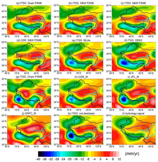
Figure 4.
Same as Figure 1 but for some selected GRACE solutions and destriping filters smoothed by a 340-km-radius Gaussian filter (a–j), compared with the signals from the ITSG solution without destriping (k) and aggregated hydrology signals (l), but smoothed by the same Gaussian filter. The Gaussian filter is not used for ITSG+DDK2 (f), because the DDK2 filter has the smoothing characteristics of a 340-km-radius Gaussian filter according to Kusche et al. [5]. The purple lines in (a–d) delimit the range of the the Three-River-Source Region (below) and Qaidam Basin (above), and the dark brown rectangle represents the West Kunlun region.
For comparison we show trend rates (Figure 4e–j), annual amplitudes (Figure A4e–j), and annual phases (Figure A5e–j) from the ITSG SH solutions with filter ‘MLAs’, ‘DDK2’ and ‘Cham P4M8’, and the three mascon models, with the same additional Gaussian smoothing. They have different patterns and magnitudes than those determined with the best GRACE solution-filter combinations inside and outside the plateau (e.g., Figure 4a–d). For example, in the plateau interior, the single-anomalies of the smoothed trends (Figure 4e–j) have their centers in the center of the plateau, with an exception of Figure 4g where two anomalies appear with one in the east and the other in the west. Obviously, those are different from one single positive anomaly with the center in the east as for the determined smoothed trends from the best combinations (Figure 4a–d). Such single anomalies in the center of the plateau, as found with less effective destriping filters and the three mascon models, present signal patterns with shapes and amplitudes similar to Figure 4k where destriping was omitted and the result is only smoothed by a 340-km-radius Gaussian filter. Hence, these results may result from not effectively suppressed stripe noise. These results as well as the occurrence of two anomalies (Figure 4g) are also not supported by the Gaussian filter smoothed AHS (Figure 4l).
4.3. Assessment of the Effectiveness of Destriping Filters and GRACE Solutions
We investigate the effectiveness of destriping for the tested destriping filters and three mascon models by a combined analysis of the filtered and unfiltered (Figure 1l) TWS trends.
First, we focus on the unfiltered results (Figure 1l), in which the anomalies inside and outside the plateau are elongated in the north-south direction, and thus are extremely impacted by the N-S striping noise. According to Wahr et al. [55], a Gaussian filter deals with the stochastic noises in the higher-degree Stokes coefficients, making the filtering equivalent to a spatial smoothing of the TWS trends. The N-S stripes should be one kind of system-noise errors, which should be suppressed with a dedicated destriping filter such as ‘Duan P4M8’, ‘S&W P2M8’ and ‘S&W P3M8’. Therefore, although the N-S stripes are not apparently visible in the smoothed result (Figure 4k), we cannot expect that the effects of N-S stripes are fully suppressed when only a Gaussian filter is used. We thus consider the TWS trends shown in Figure 4k, smoothed but not destriped, as a benchmark for indicating the large effects of N-S stripes.
Since N-S stripes in the TWS trends from the five best solution-filter combinations (i.e., ‘ITSG+Duan P4M8’, ‘ITSG+S&W P2M8’, ‘ITSG+S&W P3M8’, ‘CSR+Duan P4M8’ and ‘CSR+S&W P3M8’) before smoothing (Figure 1c–e and Figure 2a,b) are already almost imperceptible, the corresponding Gaussian smoothed TWS trends (Figure 4a–d) certainly show different patterns from our chosen benchmark result (Figure 4k). Note that the TWS trends from best solution-filter combinations before smoothing also agree well with the AHS (Figure 3f), showing the larger PCC- and IOA-values, and smaller RMSE-values. Figure 1c–e, Figure 2a,b and Figure 4a–d thus present reasonable GRACE-derived TWS trends before and after smoothing, respectively, in which the N-S stripes are effectively suppressed. Due to extreme similarity with those from ‘CSR+S&W P3M8’, TWS trends from ‘CSR+Duan P4M8’ are thus not shown in these Figures.
For the combination series ‘ITSG+Cham PxM8’, obvious stripes in the TWS trends before smoothing are seen in Figure 1g–i with very small PCC- and IOA-values, and very large RMSE-values. The pattern of the TWS trends after smoothing (Figure 4g) is not supported by the smoothed AHS (Figure 4l).
From the DDK series of filtered data products, we select two representative filters, DDK8 and DDK2 with weak and strong filtering, respectively. As seen in Figure 1k, the TWS trends of DDK8 are less effectively destriped, with anomalies stretched in the N-S direction visually and small PCC- and IOA-values as well as large RMSE-values. For the DDK2 filter, equivalent to a 340-km-radius Gaussian filter [5], the similarity of the derived TWS trends (Figure 4f) to the benchmark results (Figure 4k) implies that the original N-S stripes seem to be smoothed just by a Gaussian filter, but not effectively suppressed. As for the NLAs filter, although there are no obvious N-S stripes in the TWS trends before smoothing (Figure 1j), the PCC- and IOA-value are quite small, and RMSE-values are quite large. The positive anomaly inside the plateau after smoothing (Figure 4e) does not show its tail and has its center somewhat in the center of the plateau, which resembles the benchmark result (Figure 4k). Of course, this is not supported by the smoothed AHS (Figure 4l).
Larger PCC- and IOA-values, and smaller RMSE-values are achieved if GRACE SH solutions are combined with the best-performing filters ‘Duan P4M8’, ‘S&W P2M8’ and ‘S&W P3M8’ (Figure 1c–e and Figure 2a–e, Table 2 and Table A1), whereas largest values yield for ITSG and CSR (except ‘S&W P2M8’) which also match the AHS very well before and after smoothing with a Gaussian filter. When the time span is extended from ending in December 2009 to ending in December 2016, a similar performance is found for the above filters and GRACE solutions. However, the PCC-, RMSE- and IOA-values shown in Figure A6 are smaller than those for the time span 2003 to 2009. This is due to limited availability of monitoring data of glacier melting and lake water changes as well as the lack of groundwater storage changes data for the longer period until 2016.
For the three mascon models, the anomalies inside the plateau of the TWS trends before smoothing (Figure 2f–h) cannot match the three positive anomalies and one negative anomaly (Figure 3f), which shows bad pattern agreement of the results with the AHS. In addition, as mentioned above, the anomaly patterns of the three mascon models and their magnitudes do not match with each other inside and outside the plateau. Furthermore, the smoothed TWS trends (Figure 4h–j) show very similar patterns with those of the benchmark results (Figure 4k), which strongly implies that large effects due to N-S stripes are included. This, in turn, means that, although not visible, N-S stripes have already not been effectively suppressed in the TWS trends before smoothing (Figure 2f–h). This is probably due to some smoothing functions in the inversion processing of mascons. We thus argue that the tested mascon models are less reliable in the TP area.
4.4. Additional Tests and Discussions
Although the contributions of each hydrology component in the AHS have been well determined, as a criterion for selecting, it is necessary to investigate the influence of its uncertainties on identifying the best solution-filter combination or mascon model. Therefore, we estimated the error sigmas for each contribution (Figure A7a–d) referring to Xiang et al. [2] and calculated the error sigmas () for the AHS (Figure A7e) using Equation (A4) and a square root function. Further, four extreme cases of AHS (Figure A7f–i) considering and as their uncertainties were simulated. Based on those, we conducted the same experiments as outlined in Section 4.1 but using the four extreme cases of AHS.
We can find in Figure A7e that the for AHS in the plateau interior (delimited by red lines, also in Figure 3f) are relatively small, avoiding large signal leakage from strong hydrology signals around. Therefore, when considering the four extreme cases ‘AHS ’ and ‘AHS ’, their signal patterns in Figure A7f–i are very similar to those of the AHS in Figure 3f.
The PCC-, RMSE- and IOA-values between the GRACE-derived TWS trends and the four extreme cases of AHS are listed in Table A2, Table A3, Table A4 and Table A5. In Table A2 and Table A3, the PCC-, RMSE- and IOA-values are for the cases of ‘AHS+’ and ‘AHS-’, respectively. Similar to Table 2, the larger PCC- and IOA-values and smaller RMSE-values are still obtained for combinations of destriping filters ‘Duan P4M8’, ‘S&W P2M8’ and ‘S&W P3M8’ separated by two dashed lines in the Table A2 and Table A3, while their combinations with ITSG and CSR SH models show the highest correlation and agreement. All other destriping filters and mascon solutions generally result in much smaller PCC- and IOA-values, and much larger RMSE-values. This confirms the selected solutions and destriping filters in our study and verifies the effectiveness of our designed AHS criterion.
The variation of AHS leads to only small changes in PCC-values, but alters both RMSE- and IOA-values remarkably clearly (Table A2 and Table A3). The PCC-value describes consistent proportional increases or decreases around the respective means of two models but only few differences between their magnitudes [59], thus reflecting mainly the similarity of signal distribution. Changes of in AHS do not change the signal pattern much (Figure A7f,g), thus the PCC-value is not altered much, but they change the differences between the observed signals and the AHS. These differences affect RMSE- and IOA-values, however, and thus they change somewhat significantly. The ‘AHS+’ case (Table A2) yields smaller RMSE-values and better IOA agreement than the AHS, while the ‘AHS-’ case (Table A3) results in larger RMSE-values and worse IOA agreement than the AHS. That means the ‘AHS+’ would be closer to the TWS changes actually happening in the interior of the TP than the AHS, and much closer than the ‘AHS-’ case. When adding or subtracting from AHS, the ‘AHS-’ case (Table A5) performs even worse than the ‘AHS-’ case, while in the ‘AHS+’ case (Table A4), the indicator values provided both better and worse agreement than the AHS for different solutions and indicators used. These differing results of the cases may be due to the absence of groundwater increase in the TP [2] contributing to the AHS. This hypothesis should be addressed in a future study.
Concerning the validity of the SH solution and mascon models in the TP, Figure 2 shows striking disagreements between SH solutions and mascon models. TWS changes from the three mascon models do not reflect changes of soil moisture, glacier, lake water and permafrost in the interior of the TP. Mascon models appear to be applicable only to regions with simple or easily-distinguishable and large TWS changes, but our investigations show that they are not applicable to the TP where complex components contributions (e.g., soil moisture, glaciers, lakes, permafrost and groundwater) distributed in various places constitute the TWS changes, especially when parts are difficult to observe independent of GRACE, such as groundwater and permafrost [2].
The JPL_M mascon model takes advantage of near-global geophysical models to prevent longitudinal ‘stripe patterns’ in the solutions which are caused by GRACE’s poor observability of east-west gradients [48]. While the GLDAS NOAH model is the only hydrological constraint used in the TP [48], GLDAS NOAH neither defines the ice-covered region nor depicts the sites and distribution of the lakes and other components contributions [25], which introduces regional errors. JPL_M uses equal-area spherical cap mascons, each usually covering an area with scattered small lakes, glaciers, permafrost, unknown groundwater and/or other components, which yield the large total water changes. As a mascon consists of a flat disk mascon unit mass, it is, in essence, a form of isotropic smoothing filter which removes longitudinal stripe patterns quite effectively visually, but in reality, it smoothes both stripe errors and the actual signal simultaneously. This explains the similarity of signal patterns between smoothed TWS trends (Figure 4i) and those of the benchmark results (Figure 4k).
CSR_M is developed with resolution hexagonal tiles mascons, based on regularized spherical harmonic GRACE solutions derived from GRACE information only [6]. The developers emphasize that the regularized spherical harmonic solutions benefit from the L-curve method with Tikhonov regularization, significantly reducing striping errors [6,60]. GSFC_M provides global mascon solution with resolution, resulting from an approach that combines an iterative solution strategy with specially designed regularization matrices for the mascon inversion, which is also reported to be highly effective by the developers [49]. Although CSR_M and GSFC_M are successfully used in many regions [6], the destriping effectiveness of their inversion processing is not supported in the TP given our results above.
As we know, some GRACE SH solutions provide Stokes coefficients d/o up to 96 (e.g., CSR) or even 120 (i.e., ITSG). In order to investigate the effects of higher d/o Stokes coefficients (e.g., from 61 to 90) on the GRACE-derived TWS changes, we conducted the same experiments as mentioned above in Section 3 and Section 4 but using Stokes coefficients maximum d/o up to 90, and show corresponding results in Figure A8, Figure A9 and Figure A10.
It is found that nearly all results show obvious N-S stripes in the TWS trends from GRACE SH solutions regardless of different destriping filters applied (Figure A8, with exception of Figure A8c,f) or different SH solutions (Figure A9a–e). All the results show poor pattern and magnitude agreements with the AHS (Figure A10f). Thus, rather low PCC- and IOA-values and rather high RMSE-values are expected, which implies heavy N-S stripe noises in the TWS change trends. In other words, current destriping filters cannot depress the N-S stripes effectively for Stokes coefficients of higher d/o (i.e., 60–90). The destriping filters Cham PxM8 (x = 2,3,4) showed the worst effectiveness in depressing N-S stripes, because the related TWS trends (Figure A8g–i) resemble the pattern of unfiltered results (Figure A8l), showing nearly no valid signal at all.
Although there are no stripes found in the TWS trends from the three mascon solutions with higher d/o (Figure A9f–h), all PCC-, RMSE- and IOA-values between the GRACE TWS signals and the AHS (Figure A10f) suggest a strong influence of N-S stripes remaining.
Although this paper is devoted to the determination of the GRACE-derived TWS changes inside the plateau, Figure 1, Figure 2 and Figure 4 show that the TWS changes outside the plateau also strongly vary depending on the selected destriping filters as well as GRACE solutions. It appears that our best GRACE solution-filter combinations for the area inside the plateau could still be applicable for the areas outside the plateau. Hence, determined TWS changes there, as shown in Figure 1c–e, Figure 2a,b and Figure 4a–d, would reasonably reflect the glacier melting in the surrounding mountains of the Tien Shan, Himalayas and southeast of the plateau, as well as the over-exploitation of groundwater from Northwest India to the Bengal Basin. Note that the determined TWS changes outside the plateau also have similar characteristics of patterns and magnitudes in all best GRACE solution-filter combinations.
In view of the fact that GRACE Follow-On (GRACE-FO) data are of the same type and format as GRACE data, and are affected by the same sources of error, our findings above are considered to be applicable to GRACE-FO missions too. Several studies show, meanwhile, the excellent continuation of the GRACE data with GRACE-FO data [61,62]. GRACE-FO data are not included in this study due to limited availability of AHS components which hinders the extension of our investigation time span to the whole period of GRACE and GRACE-FO together.
Our results of the GRACE-derived TWS changes could be influenced by signal leakages due to the truncation of higher harmonic degree terms and necessary filtering (e.g., using a Gaussian filter in this study). However, it is beyond the scope of this study to remove the leakage effects to restore the realistic signals of TWS changes. Concerning the solid earth dynamics in the TP and adjacent areas, we corrected the effect of GIA on the GRACE-derived TWS changes with the GIA model ICE-6G_C(VM5a) carefully. The broad-scale tectonic uplift in the TP would be isostatically compensated by an increasing mass deficiency at depth and has little net effects on our results [63], while the erosion rates are too small and conservative [2]. Both effects are thus not considered in this study.
5. Conclusions
We identified the best GRACE solution-filter combination for identification of terrestrial water storage changes in the Tibetan Plateau. ‘Duan P4M8’, ‘S&W P2M8’ and ‘S&W P3M8’ are found to be best destriping filters as they remove the spatially correlated errors for all twelve GRACE SH solutions tested in here. These three destriping filters, together with the two GRACE SH solutions of ITSG and CSR, can be considered the best solution-filter combinations, since the inversed TWS changes from 2003 to 2009 inside the Tibetan Plateau agree well with the aggregated hydrology signals, with an exception of the CSR solution together with the ‘S&W P2M8’ filter. This is also confirmed when extending the end of the time span from 2009 to 2016.
The TWS changes, including trends and annual signals with and without smoothing by a 340-km-radius Gaussian filter, are well determined with our best GRACE solution-filter combinations, which yield very similar features in the signal pattern and very similar magnitudes inside and outside the plateau. We find three positive anomalies and two negative TWS trend anomalies inside the plateau which can also be identified in an aggregated hydrology signal. Inspection of smoothed results shows one single anomaly inside the plateau, elongated from east to west with its center in the east of the plateau and a small tail showing slight increase in the West Kunlun region, as found by Jiao et al. [16] and Xiang et al. [2,53]. We suggest that the best solution-filter combinations can also be applied to the areas outside the plateau and other observation time spans, and thus can help to reasonably determine TWS changes inside and outside the plateau during the GRACE lifetime from 2002 to 2017, as well as its Follow-On (GRACE-FO) mission.
Very different TWS changes inside and outside the plateau from those found with our best solution-filter combinations are derived with the Chambers, DDK8/DDK2 and MLAs filters, as well as the three mascon models. We think this is very likely due to the fact that the N-S stripes are not effectively suppressed, and thus these filters and products are recommended to be used only very carefully when investigating TWS changes in the Tibetan Plateau and adjacent areas.
Finally, noting that current destriping filters cannot depress the N-S stripes effectively for Stokes coefficients of d/o higher than 60, Stokes coefficients of only d/o 1-60 of GRACE SH solutions are suggested to be used for investigation of TWS changes.
Author Contributions
Conceptualization, L.X. and H.W.; methodology, L.X.; software, L.X.; validation, L.X., B.Q.; L.J. and P.G.; formal analysis, L.X. and H.S.; investigation, L.X.; L.J. and P.G.; resources, L.X.; H.S. and W.F.; data curation, L.X.; writing—original draft preparation, L.X. and H.W.; writing—review and editing, L.X.; H.W.; H.S.; B.Q.; L.J.; W.F. and P.G.; visualization, L.X.; supervision, H.W. and H.S.; project administration, L.X.; funding acquisition, L.X.; H.W. and B.Q. All authors have read and agreed to the published version of the manuscript.
Funding
This research was funded by the National Key R & D Program of China (2017YFA0603103), the National Natural Science Foundation of China (42004007, 41901078, 41974009), the Key Research Program of Frontier Sciences, Chinese Academy of Sciences (QYZDB-SSW-DQC027, QYZDJ-SSW-DQC042), and the open fund of State Key Laboratory of Geodesy and Earth’s Dynamics, Innovation Academy for Precision Measurement Science and Technology, CAS (SKLGED2021-2-6).
Institutional Review Board Statement
Not applicable.
Informed Consent Statement
Not applicable.
Data Availability Statement
The data underlying this article are available in the article and in its online supplementary material. Twelve GRACE SH solutions (ITSG/CSR/COST-G/JPL/GFZ/Tongji/WHU/HUST/GRGS/IGG/AIUB/XISM) and the filtered results with DDK2/DDK8 are available on the website of the International Centre for Global Earth Models (ICGEM) (http://icgem.gfz-potsdam.de/series, accessed on 5 February 2021). The mascon model can be obtained from http://www2.csr.utexas.edu/grace/RL06_mascons.html, the mascon model JPL_M from https://grace.jpl.nasa.gov/data/get-data/jpl_global_mascons/, and the mascon model GSFC_M from https://earth.gsfc.nasa.gov/geo/data/grace-mascons. Degree-1 and C20 data are available via GRACE TN-13 (GRACE Technical Note 13, https://podaac-tools.jpl.nasa.gov/drive/files/allData/grace/docs/TN-13_GEOC_CSR_RL06.txt) and GRACE TN-14 (NASA GSFC SLR C20 and C30 solutions, https://podaac-tools.jpl.nasa.gov/drive/files/allData/grace/docs/TN-14_C30_C20_GSFC_SLR.txt), respectively. The ICE-6G_C model is available at http://www.atmosp.physics.utoronto.ca/~peltier/data.php.
Acknowledgments
We thank three anonymous reviewers and the academic editor for their careful reading and insightful comments and suggestions which helped us to improve the manuscript. We thank Dimitrios Piretzidis for providing data processed with the ‘MLAs’ method. Guoqing Zhang and Xingdong Li are also thanked for kindly supplying lake water changes data.
Conflicts of Interest
The authors declare no conflict of interest.
Appendix A
Appendix A.1. PCC-Value, RMSE-Value and IOA-Value
Pearson’s correlation coefficient is one of the methods widely used for evaluating the strength of relationship between two vectors [64]. However, Pearson’s correlation coefficient is not sensitive to differences between the observed signals and the aggregated hydrology signals (AHS) [59,65]. Therefore, the frequently used difference-based indicator Root Mean Square Error is also implemented to show the averaged difference. However, Root Mean Square Error does not reflect the relative size and the nature (type) of the average differences [65]. The relative and bounded indicator ‘Index of Agreement’ is thus used, which can make cross-comparisons between observed and aggregated models [65]. So, in this paper, the three methods are used together to evaluate the degree of agreement between GRACE-derived trends of TWS changes and the AHS. Pearson’s correlation coefficients (PCC-values), Root Mean Square Errors (RMSE-values), and Index of Agreement values (IOA-values) can be expressed with Equation (A1)–(A3), respectively.
where is the covariance of trends of TWS changes and AHS on grids, while and are the corresponding variance, respectively.
and
where and are the trends of TWS and AHS on grids, n is the number of grids in target area, and is the mean of all .
The PCC-value always has values between −1 and 1. A value of ±1 indicates a perfect degree of association between the two variables, a + (plus) sign indicates a positive relationship and a − (minus) sign indicates a negative relationship. When the correlation coefficient value approaches 0, the relationship between the two variables will be weaker. The RMSE-value summarizes the mean difference in the units of the observed and aggregated signals, which is a measure of how much the differences between the models are spread out. The IOA-value ranges from 0 to 1. The closer the IOA-value is to 1, the better the model-data agreement is.
Appendix A.2. Error Estimation of the Aggregated Hydrology Signal
The AHS in this paper are derived from soil moisture (SM), glacier ice (ICE), lake water (LAKE) and permafrost (PM). Therefore, the error variances () for the AHS can be calculated by
Referring to Xiang et al. [2], error sigmas at grids for SM () are given by the standard error of the mean (SEM) of Noah, VIC and CLSM models, error sigmas for ICE () are calculated with uncertainties of glacier regions provided by Gardner et al. [28], while those for LAKE () and PM () are given by absolute values of 10 and 100 percent of the signals, respectively.
Appendix A.3. Complementary Figures and Tables

Figure A1.
(a,b) are the same as Figure 1a–c, but for the destriping filters (a) ‘Duan P4M10’ and (b) ‘Duan P4M15’, while (c,d) are the same as Figure 1d–f, but for the destriping filters (c) ‘S&W P3M10’ and (d) ‘S&W P3M15’.
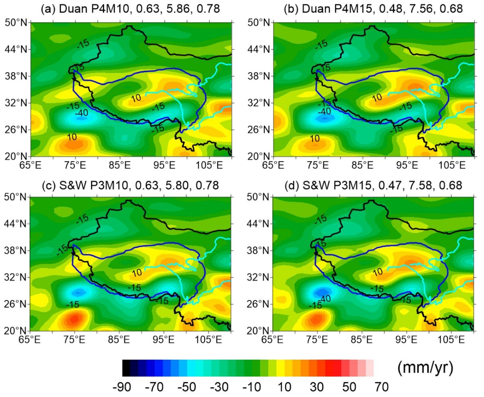
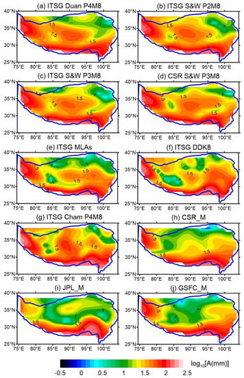
Figure A2.
Annual amplitudes of the TWS changes from 2003 to 2009 in the plateau interior for selected GRACE solutions and destriping filters.
Figure A2.
Annual amplitudes of the TWS changes from 2003 to 2009 in the plateau interior for selected GRACE solutions and destriping filters.
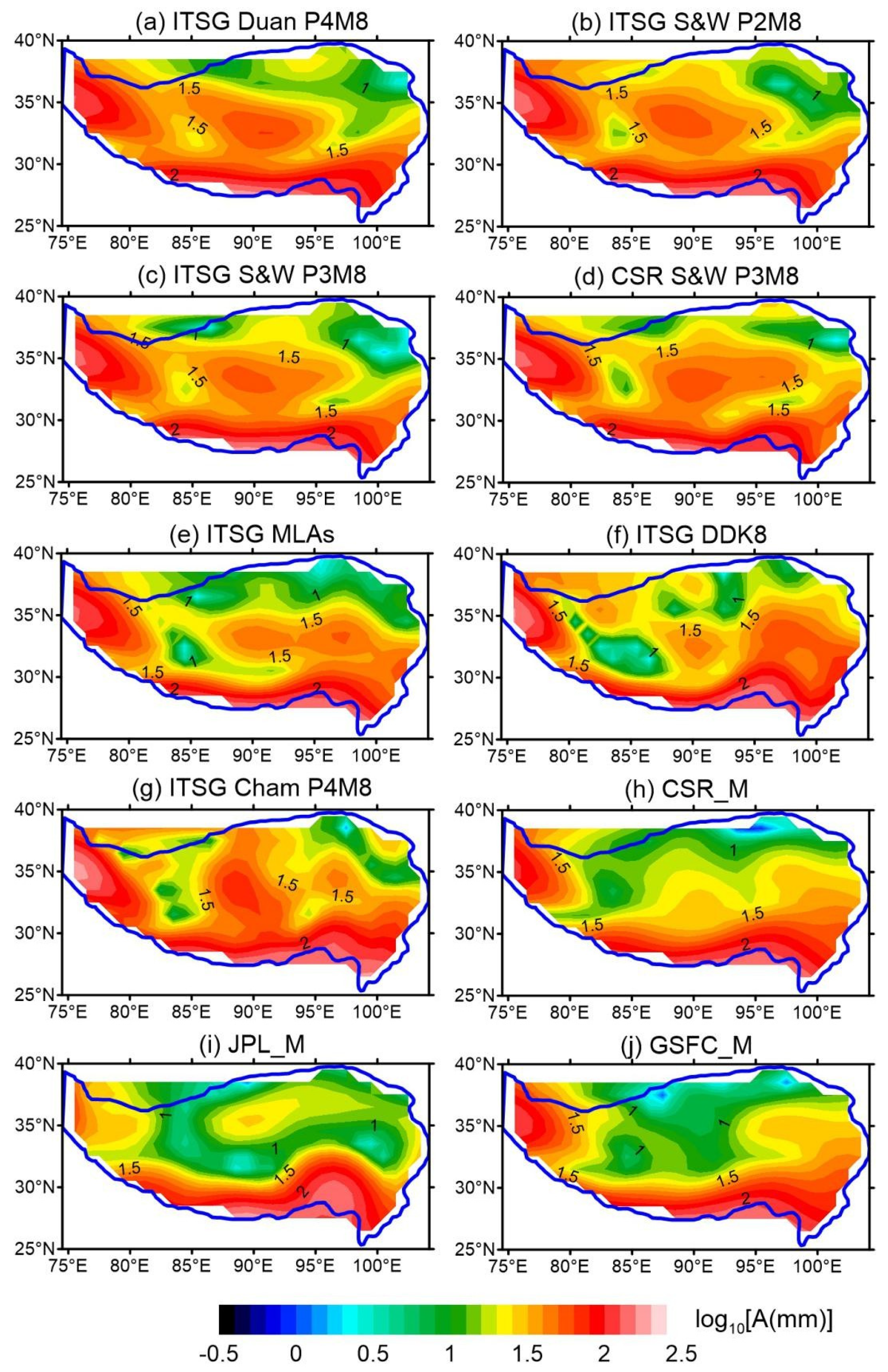
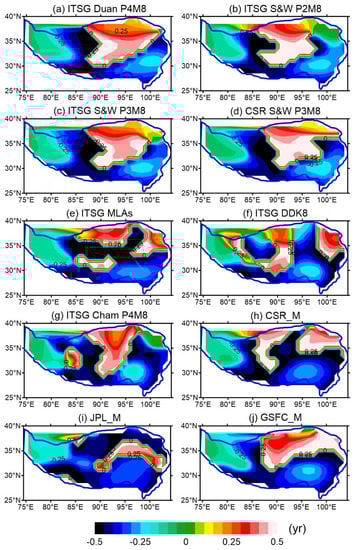
Figure A3.
Annual phases of the TWS changes from 2003 to 2009 in the plateau interior for selected GRACE solutions and destriping filters.
Figure A3.
Annual phases of the TWS changes from 2003 to 2009 in the plateau interior for selected GRACE solutions and destriping filters.

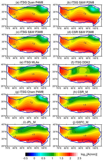
Figure A4.
Same as Figure A2 but additionally smoothed by a 340-km-radius Gaussian filter. The Gaussian filter is not used for ITSG+DDK2 (f).
Figure A4.
Same as Figure A2 but additionally smoothed by a 340-km-radius Gaussian filter. The Gaussian filter is not used for ITSG+DDK2 (f).
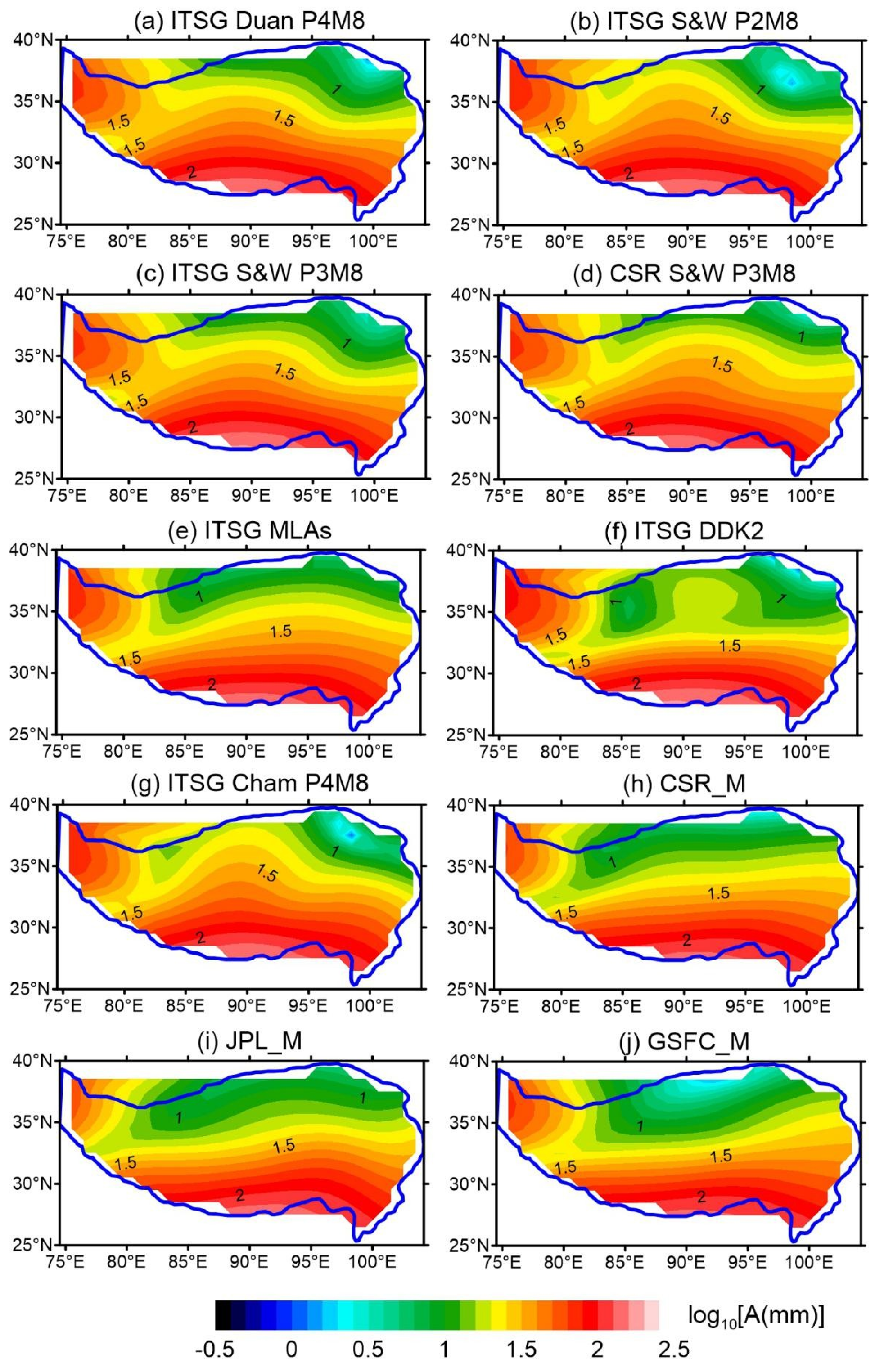
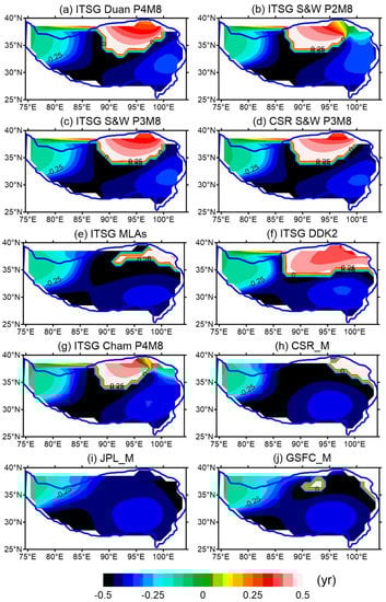
Figure A5.
Same as Figure A3 but additionally smoothed by a 340-km-radius Gaussian filter. The Gaussian filter is not used for ITSG+DDK2 (f).
Figure A5.
Same as Figure A3 but additionally smoothed by a 340-km-radius Gaussian filter. The Gaussian filter is not used for ITSG+DDK2 (f).
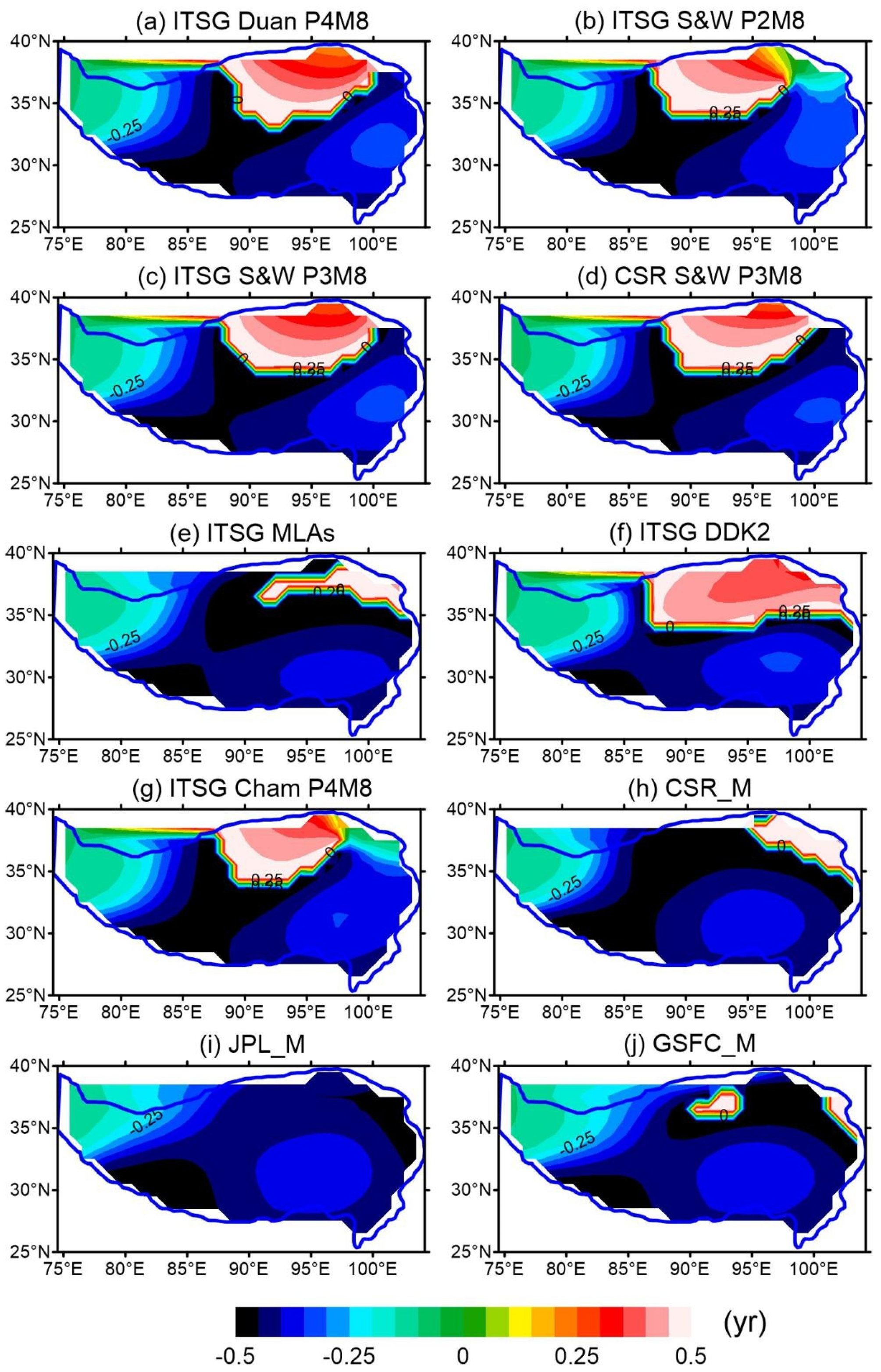
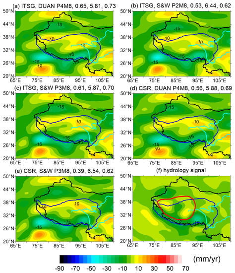
Figure A6.
Trend rates of the TWS changes derived from the best solution-filter combinations (a–e) and SH trend rates of the aggregated hydrology signals (f) from 2002 to 2016 in the Tibetan Plateau and adjacent areas, which are also derived from the SH coefficients truncated at d/o 60.
Figure A6.
Trend rates of the TWS changes derived from the best solution-filter combinations (a–e) and SH trend rates of the aggregated hydrology signals (f) from 2002 to 2016 in the Tibetan Plateau and adjacent areas, which are also derived from the SH coefficients truncated at d/o 60.

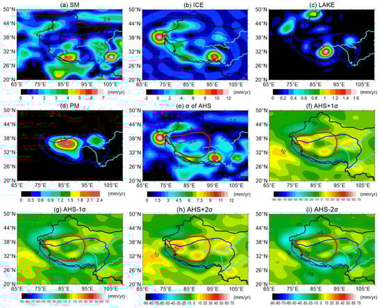
Figure A7.
Error sigmas for hydrology components (a–d) and the aggregated hydrology signals (AHS) (e), and four extreme cases of AHS considering and (f–i) as their uncertainties. Error sigmas represent square roots of the error variances for the AHS.
Figure A7.
Error sigmas for hydrology components (a–d) and the aggregated hydrology signals (AHS) (e), and four extreme cases of AHS considering and (f–i) as their uncertainties. Error sigmas represent square roots of the error variances for the AHS.
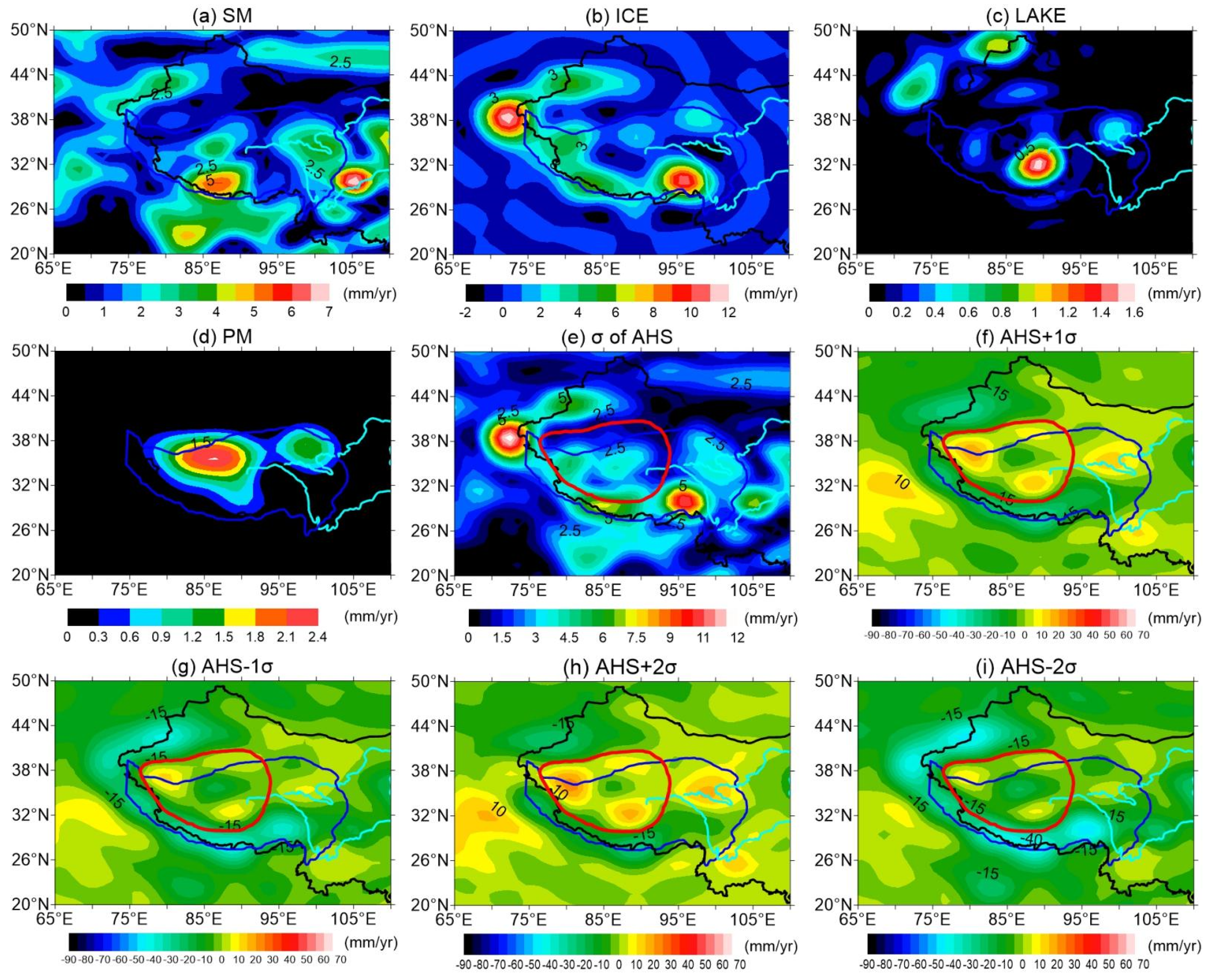
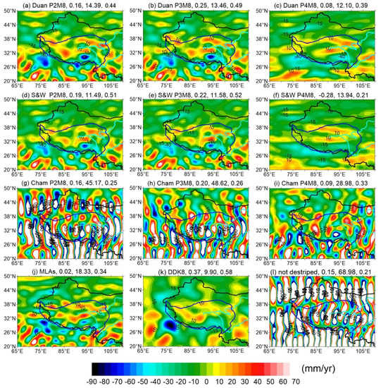
Figure A8.
Same as Figure 1 but for the ITSG GRACE solution truncated at d/o 90.
Figure A8.
Same as Figure 1 but for the ITSG GRACE solution truncated at d/o 90.
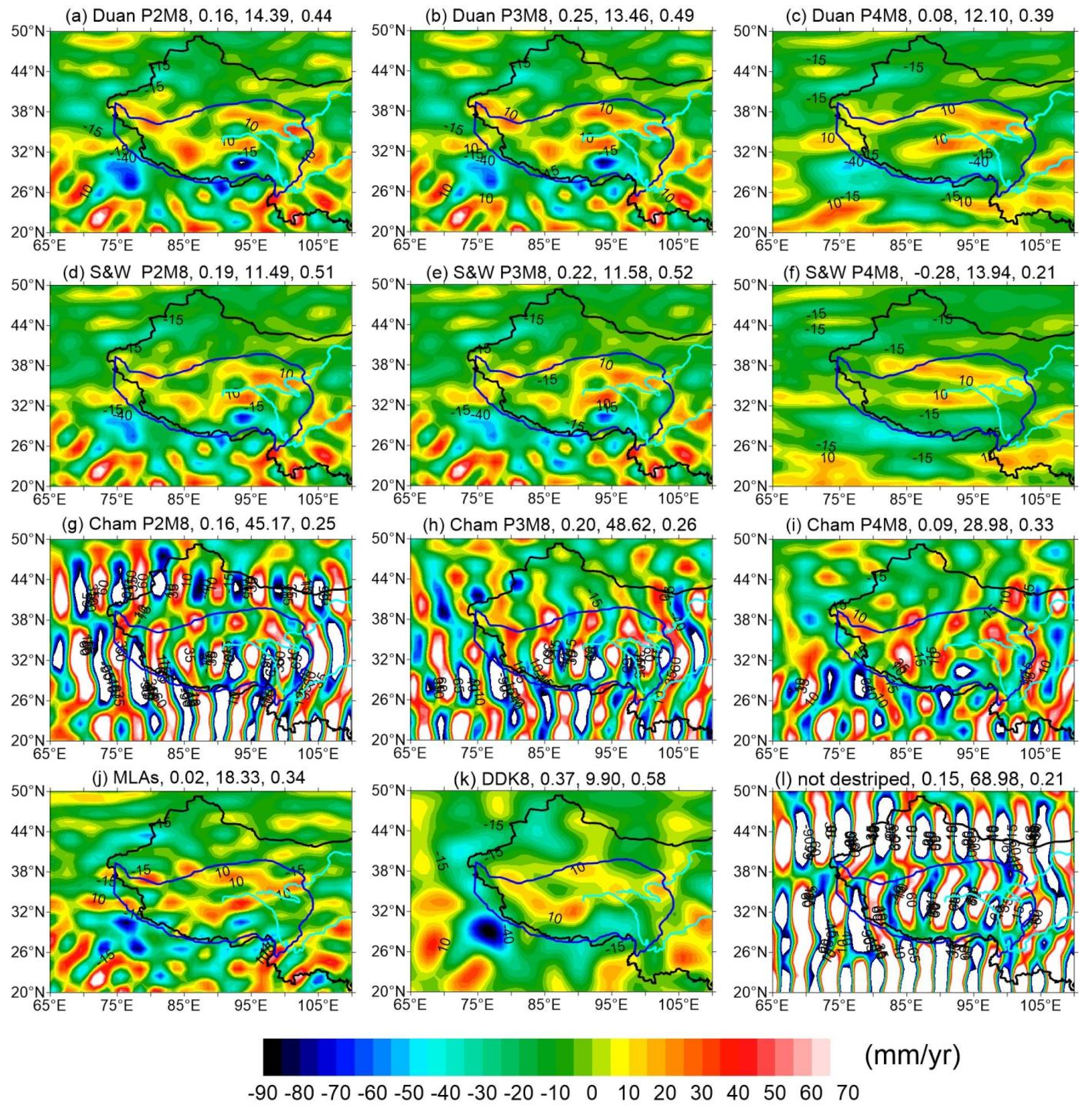
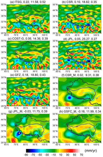
Figure A9.
Same as Figure 2 but for the Stokes coefficients from SH solutions and decomposed from three mascon models truncated at d/o 90.
Figure A9.
Same as Figure 2 but for the Stokes coefficients from SH solutions and decomposed from three mascon models truncated at d/o 90.
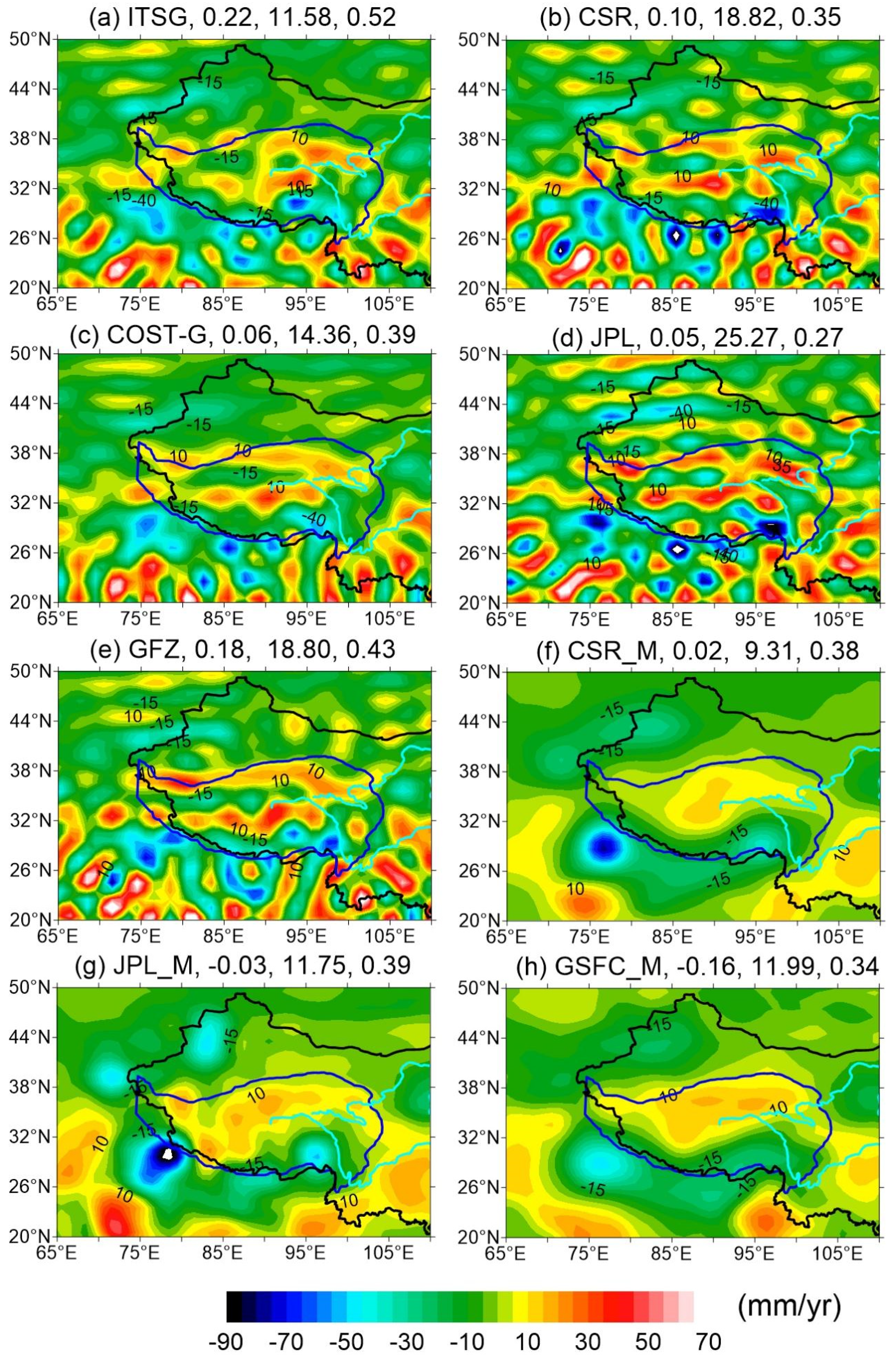
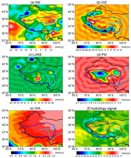
Figure A10.
Same as Figure 3 but for the SH coefficients truncated at d/o 90.
Figure A10.
Same as Figure 3 but for the SH coefficients truncated at d/o 90.
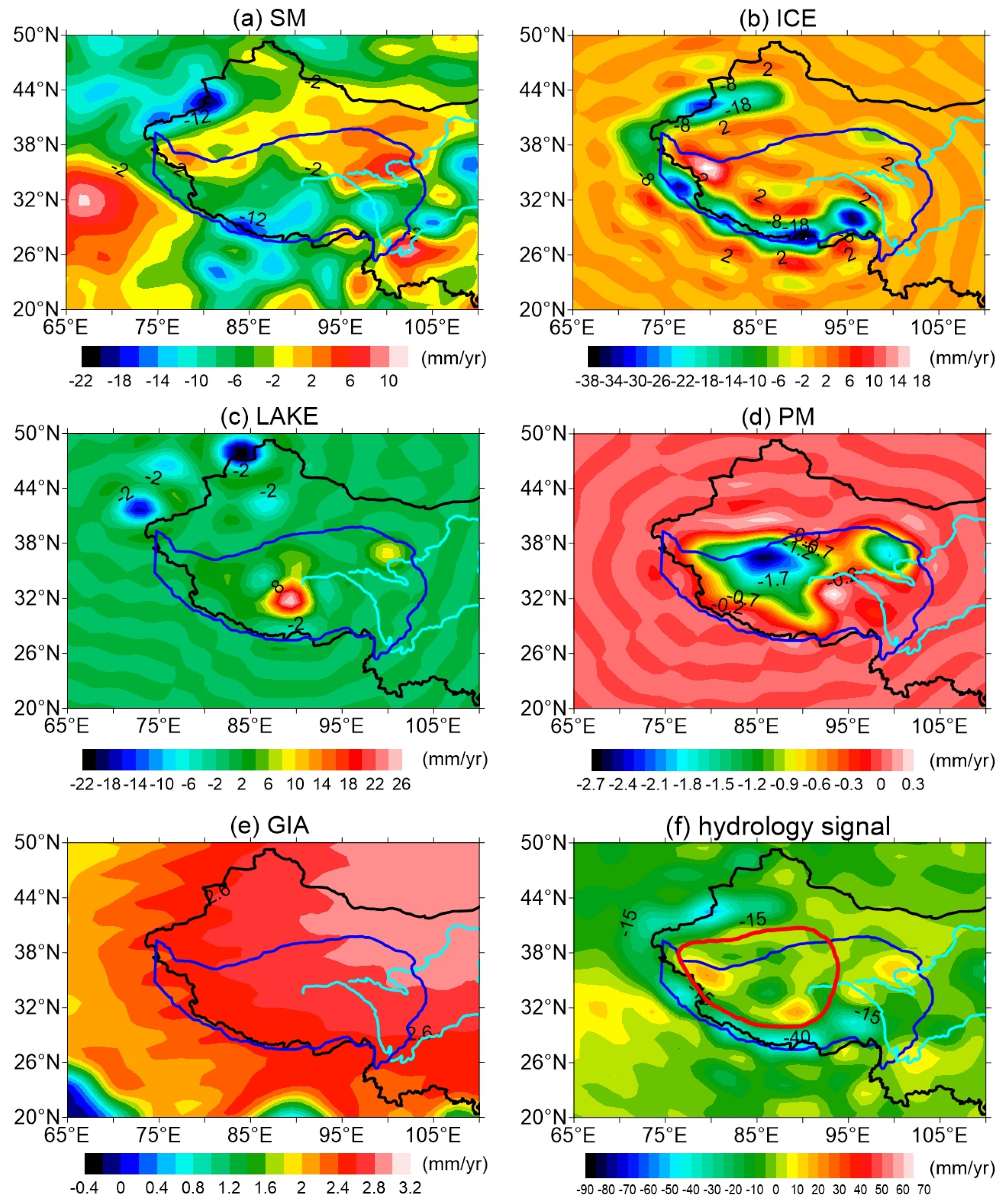
Table A1.
Same as Table 2 but for GRACE-derived TWS trends derived from the other 7 different GRACE SH solutions.
Table A1.
Same as Table 2 but for GRACE-derived TWS trends derived from the other 7 different GRACE SH solutions.
| Destriping Filters | Tongji | WHU | HUST | GRGS | ||||||||
| PCC | RMSE | IOA | PCC | RMSE | IOA | PCC | RMSE | IOA | PCC | RMSE | IOA | |
| Duan P2M8 | 0.27 | 9.09 | 0.53 | 0.28 | 8.92 | 0.55 | 0.26 | 9.85 | 0.53 | 0.38 | 9.76 | 0.58 |
| Duan P3M8 | 0.47 | 7.20 | 0.65 | 0.49 | 6.87 | 0.68 | 0.44 | 8.05 | 0.62 | 0.51 | 8.57 | 0.64 |
| Duan P4M8 | 0.58 | 5.69 | 0.71 | 0.55 | 5.77 | 0.70 | 0.62 | 5.83 | 0.75 | 0.57 | 6.79 | 0.70 |
| S&W P2M8 | 0.56 | 5.86 | 0.66 | 0.54 | 5.89 | 0.67 | 0.51 | 6.49 | 0.65 | 0.61 | 6.78 | 0.68 |
| S&W P3M8 | 0.57 | 5.77 | 0.71 | 0.54 | 5.90 | 0.70 | 0.53 | 6.38 | 0.69 | 0.63 | 6.48 | 0.72 |
| S&W P4M8 | 0.09 | 8.15 | 0.43 | 0.05 | 8.06 | 0.39 | 0.17 | 8.06 | 0.47 | 0.15 | 8.30 | 0.45 |
| Cham P2M8 | 0.27 | 11.35 | 0.52 | 0.12 | 12.50 | 0.41 | −0.23 | 18.95 | 0.28 | 0.28 | 10.39 | 0.50 |
| Cham P3M8 | 0.27 | 10.69 | 0.52 | 0.12 | 12.71 | 0.42 | −0.21 | 18.12 | 0.30 | 0.27 | 10.75 | 0.50 |
| Cham P4M8 | 0.33 | 9.67 | 0.55 | 0.12 | 13.46 | 0.42 | −0.16 | 16.00 | 0.31 | 0.28 | 10.77 | 0.51 |
| notdestriped | 0.30 | 11.83 | 0.54 | 0.15 | 11.58 | 0.45 | −0.20 | 16.97 | 0.28 | 0.21 | 10.68 | 0.47 |
| Destriping Filters | IGG | AIUB | XISM | |||||||||
| PCC | RMSE | IOA | PCC | RMSE | IOA | PCC | RMSE | IOA | ||||
| Duan P2M8 | 0.28 | 10.42 | 0.54 | 0.22 | 9.51 | 0.51 | 0.24 | 9.70 | 0.51 | |||
| Duan P3M8 | 0.39 | 8.82 | 0.60 | 0.43 | 7.50 | 0.62 | 0.36 | 8.30 | 0.57 | |||
| Duan P4M8 | 0.50 | 6.65 | 0.69 | 0.45 | 6.44 | 0.62 | 0.46 | 6.96 | 0.67 | |||
| S&W P2M8 | 0.41 | 7.26 | 0.61 | 0.48 | 6.36 | 0.62 | 0.39 | 7.18 | 0.60 | |||
| S&W P3M8 | 0.55 | 6.34 | 0.70 | 0.50 | 6.32 | 0.66 | 0.51 | 6.42 | 0.69 | |||
| S&W P4M8 | 0.22 | 7.80 | 0.50 | 0.06 | 8.40 | 0.41 | 0.27 | 7.39 | 0.52 | |||
| Cham P2M8 | −0.04 | 16.33 | 0.35 | 0.07 | 21.65 | 0.33 | −0.07 | 16.51 | 0.35 | |||
| Cham P3M8 | 0.12 | 13.71 | 0.45 | 0.05 | 13.77 | 0.39 | 0.05 | 13.31 | 0.42 | |||
| Cham P4M8 | 0.36 | 9.85 | 0.58 | 0.03 | 13.15 | 0.41 | 0.36 | 9.83 | 0.59 | |||
| notdestriped | 0.20 | 17.24 | 0.43 | 0.17 | 14.42 | 0.45 | 0.00 | 16.78 | 0.36 | |||
Table A2.
Same as Table 2 but for the ‘AHS+’ case instead of aggregated hydrology signals (AHS).
Table A2.
Same as Table 2 but for the ‘AHS+’ case instead of aggregated hydrology signals (AHS).
| Destriping Filters | ITSG | CSR | COST-G | JPL | GFZ | ||||||||||
|---|---|---|---|---|---|---|---|---|---|---|---|---|---|---|---|
| PCC | RMSE | IOA | PCC | RMSE | IOA | PCC | RMSE | IOA | PCC | RMSE | IOA | PCC | RMSE | IOA | |
| Duan P2M8 | 0.45 | 8.43 | 0.66 | 0.43 | 8.61 | 0.64 | 0.43 | 8.40 | 0.65 | 0.37 | 9.91 | 0.60 | 0.46 | 9.29 | 0.64 |
| Duan P3M8 | 0.58 | 6.90 | 0.74 | 0.58 | 6.72 | 0.74 | 0.58 | 6.64 | 0.74 | 0.50 | 8.26 | 0.67 | 0.58 | 7.71 | 0.72 |
| Duan P4M8 | 0.64 | 5.48 | 0.79 | 0.66 | 5.13 | 0.80 | 0.62 | 5.41 | 0.78 | 0.64 | 5.26 | 0.80 | 0.60 | 6.46 | 0.76 |
| S&W P2M8 | 0.66 | 5.04 | 0.80 | 0.65 | 5.12 | 0.78 | 0.65 | 5.16 | 0.78 | 0.62 | 5.44 | 0.77 | 0.60 | 6.24 | 0.75 |
| S&W P3M8 | 0.64 | 5.41 | 0.79 | 0.65 | 5.13 | 0.80 | 0.63 | 5.36 | 0.78 | 0.64 | 5.25 | 0.79 | 0.59 | 6.36 | 0.76 |
| S&W P4M8 | 0.15 | 7.70 | 0.46 | 0.13 | 7.64 | 0.46 | 0.13 | 7.67 | 0.45 | 0.14 | 7.45 | 0.44 | 0.18 | 8.13 | 0.49 |
| Cham P2M8 | 0.04 | 13.83 | 0.37 | −0.18 | 18.65 | 0.25 | 0.00 | 13.98 | 0.35 | 0.19 | 14.31 | 0.44 | −0.11 | 24.74 | 0.25 |
| Cham P3M8 | 0.05 | 13.78 | 0.39 | −0.17 | 19.03 | 0.26 | 0.01 | 13.65 | 0.38 | 0.11 | 13.89 | 0.43 | −0.11 | 18.65 | 0.31 |
| Cham P4M8 | 0.05 | 13.85 | 0.39 | −0.02 | 15.03 | 0.35 | 0.07 | 12.91 | 0.43 | 0.21 | 13.31 | 0.48 | 0.00 | 15.66 | 0.39 |
| MLAs | 0.21 | 7.71 | 0.52 | 0.48 | 6.42 | 0.64 | - | - | - | 0.37 | 7.14 | 0.59 | 0.18 | 10.09 | 0.48 |
| DDK8 | 0.40 | 7.49 | 0.62 | −0.05 | 11.06 | 0.37 | - | - | - | 0.35 | 9.42 | 0.57 | 0.08 | 11.22 | 0.45 |
| not destriped | 0.01 | 12.73 | 0.40 | −0.14 | 17.27 | 0.27 | 0.09 | 10.32 | 0.44 | 0.39 | 14.96 | 0.52 | −0.17 | 23.63 | 0.28 |
| CSR_M | JPL_M | GSFC_M | |||||||||||||
| PCC | RMSE | IOA | PCC | RMSE | IOA | PCC | RMSE | IOA | |||||||
| 0.15 | 7.58 | 0.46 | 0.01 | 9.88 | 0.40 | −0.01 | 9.85 | 0.43 | |||||||
Table A3.
Same as Table A2 but for the ‘AHS-’ case.
Table A3.
Same as Table A2 but for the ‘AHS-’ case.
| Destriping Filters | ITSG | CSR | COST-G | JPL | GFZ | ||||||||||
|---|---|---|---|---|---|---|---|---|---|---|---|---|---|---|---|
| PCC | RMSE | IOA | PCC | RMSE | IOA | PCC | RMSE | IOA | PCC | RMSE | IOA | PCC | RMSE | IOA | |
| Duan P2M8 | 0.32 | 11.71 | 0.53 | 0.27 | 12.20 | 0.50 | 0.30 | 11.93 | 0.51 | 0.21 | 13.56 | 0.48 | 0.36 | 12.87 | 0.53 |
| Duan P3M8 | 0.52 | 9.79 | 0.62 | 0.49 | 10.10 | 0.58 | 0.52 | 9.95 | 0.59 | 0.38 | 11.60 | 0.54 | 0.55 | 11.02 | 0.60 |
| Duan P4M8 | 0.66 | 7.34 | 0.72 | 0.66 | 7.81 | 0.68 | 0.65 | 7.85 | 0.68 | 0.60 | 8.14 | 0.66 | 0.64 | 9.12 | 0.67 |
| S&W P2M8 | 0.64 | 7.78 | 0.67 | 0.58 | 8.47 | 0.61 | 0.61 | 8.37 | 0.61 | 0.50 | 9.06 | 0.57 | 0.60 | 9.52 | 0.62 |
| S&W P3M8 | 0.69 | 7.26 | 0.73 | 0.67 | 7.79 | 0.68 | 0.67 | 7.81 | 0.68 | 0.61 | 8.05 | 0.66 | 0.66 | 8.95 | 0.68 |
| S&W P4M8 | 0.32 | 8.88 | 0.52 | 0.27 | 9.41 | 0.47 | 0.30 | 9.27 | 0.48 | 0.25 | 9.26 | 0.45 | 0.36 | 10.09 | 0.52 |
| Cham P2M8 | 0.00 | 15.80 | 0.40 | −0.15 | 20.20 | 0.35 | −0.05 | 16.32 | 0.38 | 0.03 | 17.40 | 0.39 | −0.10 | 26.21 | 0.33 |
| Cham P3M8 | 0.01 | 15.86 | 0.42 | −0.14 | 20.52 | 0.36 | −0.03 | 16.01 | 0.42 | 0.02 | 16.74 | 0.42 | −0.08 | 20.52 | 0.39 |
| Cham P4M8 | 0.02 | 15.91 | 0.43 | −0.05 | 17.18 | 0.40 | 0.02 | 15.42 | 0.44 | 0.08 | 16.38 | 0.45 | 0.01 | 17.92 | 0.44 |
| MLAs | 0.24 | 9.48 | 0.46 | 0.42 | 10.02 | 0.47 | - | - | - | 0.35 | 10.40 | 0.47 | 0.28 | 12.33 | 0.50 |
| DDK8 | 0.27 | 11.11 | 0.44 | −0.05 | 13.79 | 0.39 | - | - | - | 0.20 | 13.54 | 0.44 | 0.06 | 14.61 | 0.42 |
| not destriped | 0.07 | 14.63 | 0.45 | −0.12 | 18.91 | 0.35 | 0.08 | 13.42 | 0.41 | 0.21 | 18.32 | 0.45 | −0.10 | 25.10 | 0.38 |
| CSR_M | JPL_M | GSFC_M | |||||||||||||
| PCC | RMSE | IOA | PCC | RMSE | IOA | PCC | RMSE | IOA | |||||||
| 0.11 | 10.58 | 0.38 | −0.09 | 13.51 | 0.34 | −0.03 | 13.34 | 0.40 | |||||||
Table A4.
Same as Table A2 but for the ‘AHS+’ case.
Table A4.
Same as Table A2 but for the ‘AHS+’ case.
| Destriping Filters | ITSG | CSR | COST-G | JPL | GFZ | ||||||||||
|---|---|---|---|---|---|---|---|---|---|---|---|---|---|---|---|
| PCC | RMSE | IOA | PCC | RMSE | IOA | PCC | RMSE | IOA | PCC | RMSE | IOA | PCC | RMSE | IOA | |
| Duan P2M8 | 0.49 | 7.93 | 0.69 | 0.49 | 7.85 | 0.68 | 0.48 | 7.72 | 0.68 | 0.44 | 8.95 | 0.64 | 0.49 | 8.46 | 0.67 |
| Duan P3M8 | 0.58 | 6.95 | 0.74 | 0.59 | 6.44 | 0.76 | 0.58 | 6.44 | 0.75 | 0.53 | 7.75 | 0.70 | 0.56 | 7.29 | 0.73 |
| Duan P4M8 | 0.58 | 6.55 | 0.72 | 0.61 | 5.81 | 0.75 | 0.57 | 6.15 | 0.72 | 0.64 | 5.77 | 0.76 | 0.54 | 6.76 | 0.73 |
| S&W P2M8 | 0.64 | 5.72 | 0.76 | 0.65 | 5.32 | 0.77 | 0.63 | 5.45 | 0.75 | 0.65 | 5.31 | 0.78 | 0.57 | 6.16 | 0.75 |
| S&W P3M8 | 0.57 | 6.51 | 0.71 | 0.60 | 5.83 | 0.74 | 0.56 | 6.12 | 0.72 | 0.62 | 5.81 | 0.75 | 0.52 | 6.74 | 0.72 |
| S&W P4M8 | 0.05 | 8.62 | 0.37 | 0.04 | 8.24 | 0.38 | 0.03 | 8.37 | 0.37 | 0.07 | 8.07 | 0.36 | 0.08 | 8.55 | 0.41 |
| Cham P2M8 | 0.06 | 13.67 | 0.35 | −0.18 | 18.50 | 0.19 | 0.03 | 13.59 | 0.33 | 0.27 | 13.44 | 0.47 | −0.11 | 24.49 | 0.22 |
| Cham P3M8 | 0.07 | 13.56 | 0.37 | −0.17 | 18.91 | 0.19 | 0.03 | 13.27 | 0.33 | 0.16 | 13.19 | 0.42 | −0.13 | 18.33 | 0.26 |
| Cham P4M8 | 0.06 | 13.63 | 0.36 | 0.00 | 14.69 | 0.31 | 0.09 | 12.48 | 0.39 | 0.27 | 12.50 | 0.50 | −0.01 | 15.22 | 0.34 |
| MLAs | 0.18 | 8.30 | 0.49 | 0.48 | 6.04 | 0.67 | - | - | - | 0.36 | 6.87 | 0.60 | 0.11 | 10.07 | 0.45 |
| DDK8 | 0.45 | 6.87 | 0.68 | −0.04 | 10.64 | 0.32 | - | - | - | 0.41 | 8.14 | 0.64 | 0.08 | 10.34 | 0.44 |
| not destriped | −0.01 | 12.68 | 0.36 | −0.15 | 17.12 | 0.23 | 0.09 | 9.73 | 0.42 | 0.47 | 13.87 | 0.56 | −0.21 | 23.39 | 0.23 |
| CSR_M | JPL_M | GSFC_M | |||||||||||||
| PCC | RMSE | IOA | PCC | RMSE | IOA | PCC | RMSE | IOA | |||||||
| 0.16 | 7.41 | 0.45 | 0.06 | 8.94 | 0.41 | 0.00 | 9.02 | 0.41 | |||||||
Table A5.
Same as Table A2 but for the ‘AHS-2’ case.
Table A5.
Same as Table A2 but for the ‘AHS-2’ case.
| Destriping Filters | ITSG | CSR | COST-G | JPL | GFZ | ||||||||||
|---|---|---|---|---|---|---|---|---|---|---|---|---|---|---|---|
| PCC | RMSE | IOA | PCC | RMSE | IOA | PCC | RMSE | IOA | PCC | RMSE | IOA | PCC | RMSE | IOA | |
| Duan P2M8 | 0.26 | 13.96 | 0.48 | 0.20 | 14.53 | 0.45 | 0.23 | 14.25 | 0.46 | 0.13 | 15.87 | 0.44 | 0.31 | 15.17 | 0.48 |
| Duan P3M8 | 0.47 | 12.03 | 0.55 | 0.43 | 12.46 | 0.51 | 0.47 | 12.29 | 0.52 | 0.32 | 13.87 | 0.49 | 0.51 | 13.32 | 0.54 |
| Duan P4M8 | 0.65 | 9.52 | 0.64 | 0.64 | 10.16 | 0.59 | 0.64 | 10.13 | 0.59 | 0.55 | 10.50 | 0.56 | 0.64 | 11.34 | 0.61 |
| S&W P2M8 | 0.60 | 10.14 | 0.57 | 0.53 | 10.92 | 0.51 | 0.57 | 10.80 | 0.52 | 0.43 | 11.54 | 0.47 | 0.57 | 11.89 | 0.55 |
| S&W P3M8 | 0.68 | 9.44 | 0.65 | 0.65 | 10.13 | 0.59 | 0.67 | 10.09 | 0.60 | 0.57 | 10.40 | 0.57 | 0.66 | 11.16 | 0.61 |
| S&W P4M8 | 0.38 | 10.65 | 0.49 | 0.32 | 11.33 | 0.43 | 0.36 | 11.15 | 0.45 | 0.29 | 11.21 | 0.41 | 0.42 | 12.01 | 0.50 |
| Cham P2M8 | -0.02 | 17.43 | 0.41 | −0.14 | 21.52 | 0.38 | −0.07 | 18.08 | 0.38 | −0.04 | 19.40 | 0.37 | −0.09 | 27.37 | 0.36 |
| Cham P3M8 | -0.01 | 17.52 | 0.42 | −0.12 | 21.80 | 0.39 | −0.04 | 17.78 | 0.42 | −0.02 | 18.68 | 0.41 | −0.06 | 21.97 | 0.42 |
| Cham P4M8 | 0.00 | 17.57 | 0.43 | −0.06 | 18.83 | 0.41 | 0.00 | 17.27 | 0.44 | 0.03 | 18.40 | 0.43 | 0.02 | 19.60 | 0.45 |
| MLAs | 0.24 | 11.39 | 0.42 | 0.38 | 12.44 | 0.40 | - | - | - | 0.33 | 12.71 | 0.41 | 0.32 | 14.21 | 0.48 |
| DDK8 | 0.21 | 13.49 | 0.38 | −0.06 | 15.78 | 0.38 | - | - | - | 0.14 | 15.99 | 0.39 | 0.05 | 16.79 | 0.39 |
| not destriped | 0.08 | 16.27 | 0.45 | −0.11 | 20.30 | 0.38 | 0.07 | 15.54 | 0.38 | 0.13 | 20.41 | 0.43 | −0.06 | 26.28 | 0.41 |
| CSR_M | JPL_M | GSFC_M | |||||||||||||
| PCC | RMSE | IOA | PCC | RMSE | IOA | PCC | RMSE | IOA | |||||||
| 0.10 | 12.81 | 0.33 | −0.12 | 15.81 | 0.31 | −0.03 | 15.60 | 0.37 | |||||||
References
- Matsuo, K.; Heki, K. Time-variable ice loss in Asian high mountains from satellite gravimetry. Earth Planet. Sci. Lett. 2010, 290, 30–36. [Google Scholar] [CrossRef]
- Xiang, L.W.; Wang, H.S.; Steffen, H.; Wu, P.; Jia, L.L.; Jiang, L.M.; Shen, Q. Groundwater storage changes in the Tibetan Plateau and adjacent areas revealed from GRACE satellite gravity data. Earth Planet. Sci. Lett. 2016, 449, 228–239. [Google Scholar] [CrossRef] [Green Version]
- Swenson, S.; Wahr, J. Post-processing removal of correlated errors in GRACE data. Geophys. Res. Lett. 2006, 33, L08402. [Google Scholar] [CrossRef]
- Jekeli, C. Alternative methods to smooth the Earth’s gravity field. In Report No. 327, Reports of the Department of Geodetic Science and Surveying; Ohio State University: Columbus, OH, USA, 1981. [Google Scholar]
- Kusche, J.; Schmidt, R.; Petrovic, S.; Rietbroek, R. Decorrelated GRACE time-variable gravity solutions by GFZ, and their validation using a hydrological model. J. Geodesy 2009, 83, 903–913. [Google Scholar] [CrossRef] [Green Version]
- Save, H.; Bettadpur, S.; Tapley, B.D. High-resolution CSR GRACE RL05 mascons. J. Geophys. Res. Solid Earth 2016, 121, 7547–7569. [Google Scholar] [CrossRef]
- Scanlon, B.R.; Zhang, Z.; Save, H.; Wiese, D.N.; Landerer, F.W.; Long, D.; Longuevergne, L.; Chen, J.L. Global evaluation of new GRACE mascon products for hydrologic applications. Water Resour. Res. 2016, 52, 9412–9429. [Google Scholar] [CrossRef]
- Scanlon, B.R.; Zhang, Z.; Save, H.; Sun, A.; Schmied, H.M.; van Beek, L.P.H.; Wiese, D.N.; Wada, Y.; Long, D.; Reedy, R.C.; et al. Global models underestimate large decadal declining and rising water storage trends relative to GRACE satellite data. Proc. Natl. Acad. Sci. USA 2018, 115, E1080–E1089. [Google Scholar] [CrossRef] [Green Version]
- Huang, J.; Halpenny, J.; van der Wal, W.; Klatt, C.; James, T.; Rivera, A. Detectability of groundwater storage change within the Great Lakes Water Basin using GRACE. J. Geophys. Res. 2012, 117, 08401. [Google Scholar] [CrossRef] [Green Version]
- Wang, H.; Jia, L.; Steffen, H.; Wu, P.; Jiang, L.; Hsu, H.; Xiang, L.; Wang, Z.; Hu, B. Increased water storage in North America and Scandinavia from GRACE gravity data. Nat. Geosci. 2013, 6, 38–42. [Google Scholar] [CrossRef]
- Bonin, J.A.; Chambers, D.P. Quantifying the resolution level where the GRACE satellites can separate Greenland’s glacial mass balance from surface mass balance. Cryosphere 2015, 9, 1761–1772. [Google Scholar] [CrossRef] [Green Version]
- Feng, W.; Shum, C.K.; Zhong, M.; Pan, Y. Groundwater Storage Changes in China from Satellite Gravity: An Overview. Remote. Sens. 2018, 10, 674. [Google Scholar] [CrossRef] [Green Version]
- Jing, W.; Zhang, P.; Zhao, X. A comparison of different GRACE solutions in terrestrial water storage trend estimation over Tibetan Plateau. Sci. Rep. 2019, 9, 1765. [Google Scholar] [CrossRef] [PubMed] [Green Version]
- Erkan, K.; Shum, C.K.; Wang, L.; Guo, J.; Jekeli, C.; Lee, H.; Panero, W.R.; Duan, J.; Huang, Z.; Wang, H. Geodetic Constraints on the Qinghai-Tibetan Plateau Present-Day Geophysical Processes. Terr. Atmospheric Ocean. Sci. 2011, 22, 241–253. [Google Scholar] [CrossRef] [Green Version]
- Yi, S.; Sun, W. Evaluation of glacier changes in high-mountain Asia based on 10 year GRACE RL05 models. J. Geophys. Res. Solid Earth 2014, 119, 2504–2517. [Google Scholar] [CrossRef]
- Jiao, J.J.; Zhang, X.; Liu, Y.; Kuang, X. Increased Water Storage in the Qaidam Basin, the North Tibet Plateau from GRACE Gravity Data. PLoS ONE 2015, 10, e0141442. [Google Scholar] [CrossRef] [Green Version]
- Pan, Y.; Shen, W.-B.; Hwang, C.; Liao, C.-M.; Zhang, T.; Zhang, G. Seasonal Mass Changes and Crustal Vertical Deformations Constrained by GPS and GRACE in Northeastern Tibet. Sensors 2016, 16, 1211. [Google Scholar] [CrossRef] [Green Version]
- Guo, J.; Mu, D.; Liu, X.; Yan, H.; Sun, Z. Water Storage Changes over the Tibetan Plateau Revealed by GRACE Mission. Acta Geophys. 2016, 64, 463–476. [Google Scholar] [CrossRef] [Green Version]
- Zou, F.; Tenzer, R.; Jin, S. Water Storage Variations in Tibet from GRACE, ICESat, and Hydrological Data. Remote. Sens. 2019, 11, 1103. [Google Scholar] [CrossRef] [Green Version]
- Liu, X.; Zhao, N.; Guo, J.; Sun, Y.; Guo, B.; Mou, N. Equivalent water height changes over Qinghai-Tibet Plateau determined from GRACE with an independent component analysis approach. Arab. J. Geosci. 2020, 13, 179. [Google Scholar] [CrossRef]
- Loomis, B.D.; Richey, A.S.; Arendt, A.A.; Appana, R.; Deweese, Y.-J.C.; Forman, B.A.; Kumar, S.V.; Sabaka, T.J.; Shean, D.E. Water Storage Trends in High Mountain Asia. Front. Earth Sci. 2019, 7, 235. [Google Scholar] [CrossRef]
- Duan, X.J.; Guo, J.Y.; Shum, C.K.; van der Wal, W. On the postprocessing removal of correlated errors in GRACE temporal gravity field solutions. Journal of Geodesy 2009, 83, 1095–1106. [Google Scholar] [CrossRef] [Green Version]
- Chambers, D.P. Evaluation of new GRACE time-variable gravity data over the ocean. Geophys. Res. Lett. 2006, 33. [Google Scholar] [CrossRef]
- Bettadpur, S. UTCSR Level-2 Processing Standards Document for Level-2 Product Release 0005; GRACE 327-742, CSR-GR-12-xx; Center for Space Research University: Austin, TX, USA, 2012; p. 17. [Google Scholar]
- Rodell, M.; Houser, P.R.; Jambor, U.; Gottschalck, J.; Mitchell, K.; Meng, C.-J.; Arsenault, K.; Cosgrove, B.; Radakovich, J.; Bosilovich, M.; et al. The Global Land Data Assimilation System. Bull. Am. Meteorol. Soc. 2004, 85, 381–394. [Google Scholar] [CrossRef] [Green Version]
- Oelke, C.; Zhang, T. Modeling the Active-Layer Depth over the Tibetan Plateau. Arct. Antarct. Alp. Res. 2007, 39, 714–722. [Google Scholar] [CrossRef] [Green Version]
- Zhang, G.Q.; Yao, T.D.; Xie, H.J.; Kang, S.C.; Lei, Y.B. Increased mass over the Tibetan Plateau: From lakes or glaciers? Geophys. Res. Lett. 2013, 40, 2125–2130. [Google Scholar] [CrossRef]
- Gardner, A.S.; Moholdt, G.; Graham Cogley, J.; Wouters, B.; Arendt, A.A.; Wahr, J.; Berthier, E.; Hock, R.; Tad Pfeffer, W.; Kaser, G.; et al. A reconciled es-timate of glacier contributions to sea level rise: 2003 to 2009. Science 2013, 340, 852–857. [Google Scholar] [CrossRef] [Green Version]
- Farinotti, D.; Longuevergne, L.; Moholdt, G.; Duethmann, D.; Mölg, T.; Bolch, T.; Vorogushyn, S.; Güntner, A. Substantial glacier mass loss in the Tien Shan over the past 50 years. Nat. Geosci. 2015, 8, 716–722. [Google Scholar] [CrossRef]
- Crétaux, J.-F.; Arsen, A.; Calmant, S.; Kouraev, A.; Vuglinski, V.; Bergé-Nguyen, M.; Gennero, M.-C.; Nino, F.; Del Rio, R.A.; Cazenave, A.; et al. SOLS: A lake database to monitor in the Near Real Time water level and storage variations from remote sensing data. Adv. Space Res. 2011, 47, 1497–1507. [Google Scholar] [CrossRef]
- Bi, H.; Ma, J.; Zheng, W.; Zeng, J. Comparison of soil moisture in GLDAS model simulations and in situ observations over the Tibetan Plateau. J. Geophys. Res. Atmos. 2016, 121, 2658–2678. [Google Scholar] [CrossRef] [Green Version]
- Deng, M.; Meng, X.; Ma, Y.; An, Y. Analysis on soil moisture characteristics of tibetan plateau based on GLDAS. J. Arid. Meteorol. 2018, 36, 595–602. [Google Scholar]
- Zhang, G.; Yao, T.; Shum, C.K.; Yi, S.; Yang, K.; Xie, H.; Feng, W.; Bolch, T.; Wang, L.; Behrangi, A.; et al. Lake volume and groundwater storage variations in Tibetan Plateau’s endorheic basin. Geophys. Res. Lett. 2017, 44, 5550–5560. [Google Scholar] [CrossRef]
- Chao, N.; Chen, G.; Li, J.; Xiang, L.; Wang, Z.; Tian, K. Groundwater Storage Change in the Jinsha River Basin from GRACE, Hydrologic Models, and In Situ Data. Ground Water 2020, 58 5, 5,735–748. [Google Scholar] [CrossRef]
- Qiao, B.; Nie, B.; Liang, C.; Xiang, L.; Zhu, L. Spatial Difference of Terrestrial Water Storage Change and Lake Water Storage Change in the Inner Tibetan Plateau. Remote. Sens. 2021, 13, 1984. [Google Scholar] [CrossRef]
- Kvas, A.; Behzadpour, S.; Ellmer, M.; Klinger, B.; Strasser, S.; Zehentner, N.; Mayer-Gürr, T. ITSG-Grace2018: Overview and evaluation of a new GRACE-only gravity field time series. J. Geophys. Res. Solid Earth 2019, 124, 9332–9344. [Google Scholar] [CrossRef] [Green Version]
- Meyer, U.; Jaeggi, A.; Dahle, C.; Flechtner, F.; Kvas, A.; Behzadpour, S.; Mayer-Gürr, T.; Lemoine, J.M.; Bourgogne, S. International Combination Service for Time-variable Gravity Fields (COST-G) Monthly GRACE Series. GFZ Data Serv. 2020. [Google Scholar] [CrossRef]
- Watkins, M.M.; Yuan, D.N. JPL Level-2 Processing Standards Document for Level-2 Product Release 05.1; Jet Propulsion Laboratory–JPL, California Institute of Technology: Pasadena, CA, USA, 2014; Available online: http://icgem.gfz-potsdam.de/L2-JPL_ProcStds_v5.1.pdf (accessed on 27 October 2021).
- Dahle, C.; Flechtner, F.; Gruber, C.; König, D.; König, R.; Michalak, G.; Neumeyer, K.H. GFZ GRACE Level-2 Processing Standards Document for Level-2 Product Release 0005; Scientific Technical Report-Data; Deutsches GeoForschungsZentrum GFZ: Potsdam, Germany, 2012; Volume 12, Available online: https://gfzpublic.gfz-potsdam.de/pubman/faces/ViewItemFullPage.jsp?itemId=item_108022_6 (accessed on 27 October 2021).
- Chen, Q.; Shen, Y.; Zhang, X.; Chen, W.; Hsu, H. Tongji-GRACE01: A GRACE-only static gravity field model recovered from GRACE Level-1B data using modified short arc approach. Adv. Space Res. 2015, 56, 941–951. [Google Scholar] [CrossRef]
- Guo, X.; Zhao, Q.; Ditmar, P.; Liu, J. A new time-series of GRACE monthly gravity field solutions obtained by accounting for the colored noise in the K-Band range-rate measurements. GFZ Data Serv. 2017. [Google Scholar] [CrossRef]
- Zhou, H.; Zhou, Z.; Luo, Z. A New Hybrid Processing Strategy to Improve Temporal Gravity Field Solution. J. Geophys. Res. Solid Earth 2019, 124, 9415–9432. [Google Scholar] [CrossRef]
- Lemoine, J.M.; Biancale, R.; Reinquin, F.; Bourgogne, S.; Gégout, P. CNES/GRGS RL04 Earth gravity field models, from GRACE and SLR data. GFZ Data Serv. 2019. [Google Scholar] [CrossRef]
- Wang, C.Q.; Xu, H.Z.; Zhong, M.; Feng, W.; Ran, J.J.; Yang, F. An investigation on GRACE temporal gravity field recovery using the dynamic approach. Chin. J. Geophys. 2015, 58, 756–766. [Google Scholar]
- Meyer, U.; Jäggi, A.; Jean, Y.; Beutler, G. AIUB-RL02: An improved time-series of monthly gravity fields from GRACE data. Geophys. J. Int. 2016, 205, 1196–1207. [Google Scholar] [CrossRef] [Green Version]
- Xiao, Y.; Xia, Z.; Sun, Z.; Pang, Z. Application of an Improved Dynamic Method Baseline Method to Satellite Gravtimetry Data Processing. Geomat. Inf. Sci. Wuhan Univ. 2011, 36, 280–284. [Google Scholar]
- Peltier, W.R.; Argus, D.F.; Drummond, R. Space geodesy constrains ice-age ter-minal deglaciation: The global ICE-6G_C (VM5a) model. J. Geophys. Res. Solid Earth 2015, 120, 450–487. [Google Scholar] [CrossRef] [Green Version]
- Watkins, M.M.; Wiese, D.N.; Yuan, D.-N.; Boening, C.; Landerer, F.W. Improved methods for observing Earth’s time variable mass distribution with GRACE using spherical cap mascons. J. Geophys. Res. Solid Earth 2015, 120, 2648–2671. [Google Scholar] [CrossRef]
- Loomis, B.D.; Luthcke, S.B.; Sabaka, T.J. Regularization and error characterization of GRACE mascons. J. Geod. 2019, 93, 1381–1398. [Google Scholar] [CrossRef]
- Zhong, B.; Li, Q.; Chen, J.; Luo, Z.; Zhou, H. Improved Estimation of Regional Surface Mass Variations from GRACE Intersatellite Geopotential Differences Using a Priori Constraints. Remote. Sens. 2020, 12, 2553. [Google Scholar] [CrossRef]
- Landerer, F. Monthly Estimates of Degree-1 (Geocenter) Gravity Coefficients, Generated from GRACE (04-2002-06/2017) and GRACE—FO (06/2018 onward) RL06 Solutions, GRACE Technical Note 13, The GRACE Project, NASA Jet Propulsion Laboratory. 2021. Available online: https://podaac-tools.jpl.nasa.gov/drive/files/allData/grace/docs/TN-13_GEOC_CSR_RL06.txt (accessed on 13 June 2021).
- Loomis, B.D.; Rachlin, K.E.; Wiese, D.N.; Landerer, F.W.; Luthcke, S.B. Replacing GRACE/GRACE-FO C30 With Satellite Laser Ranging: Impacts on Antarctic Ice Sheet Mass Change. Geophys. Res. Lett. 2020, 47, e2019GL085488. [Google Scholar] [CrossRef]
- Xiang, L.; Wang, H.; Jia, L. The variability of terrestrial water storage changes in the tibetan plateau and adjacent areas retrieved by GRACE data. J. Geod. Geodyn. 2017, 37, 311–318. [Google Scholar]
- Piretzidis, D.; Sra, G.; Karantaidis, G.; Sideris, M.G.; Kabirzadeh, H. Identifying presence of correlated errors using machine learning algorithms for the selective de-correlation of GRACE harmonic coefficients. Geophys. J. Int. 2018, 215, 375–388. [Google Scholar] [CrossRef]
- Wahr, J.; Molenaar, M.; Bryan, F. Time variability of the Earth’s gravity field: Hydrological and oceanic effects and their possible detection using GRACE. J. Geophys. Res. Solid Earth 1998, 103, 30205–30229. [Google Scholar] [CrossRef]
- Wang, H.; Xiang, L.; Jia, L.; Jiang, L.; Wang, Z.; Hu, B.; Gao, P. Load Love numbers and Green’s functions for elastic Earth models PREM, iasp91, ak135, and modified models with refined crustal structure from Crust 2.0. Comput. Geosci. 2012, 49, 190–199. [Google Scholar] [CrossRef]
- Li, X.D.; Long, D.; Huang, Q.; Han, P.F.; Zhao, F.Y.; Wada, Y. A High Temporal Resolution Lake Data Set from Multisource Altimetric Missions and Landsat Archives of Water Level and Storage Changes on the Tibetan Plateau during 2000–2017. Pangaea 2019. Available online: https://doi.pangaea.de/10.1594/PANGAEA.898411 (accessed on 14 January 2021).
- Brun, F.; Berthier, E.; Wagnon, P.; Kääb, A.; Treichler, D. A spatially resolved estimate of High Mountain Asia glacier mass balances from 2000 to 2016. Nat. Geosci. 2017, 10, 668–673. [Google Scholar] [CrossRef]
- Willmott, C.J. On the validation of models. Phys. Geogr. 1981, 2, 184–194. [Google Scholar] [CrossRef]
- Save, H.; Bettadpur, S.; Tapley, B.D. Reducing errors in the GRACE gravity solutions using regularization. J. Geodesy 2012, 86, 695–711. [Google Scholar] [CrossRef]
- Boergens, E.; Güntner, A.; Dobslaw, H.; Dahle, C. Quantifying the Central European droughts in 2018 and 2019 with GRACE Follow-On. Geophys. Res. Lett. 2020, 47, e2020GL087285. [Google Scholar] [CrossRef]
- Velicogna, I.; Mohajerani, Y.; Geruo, A.; Landerer, F.; Mouginot, J.; Noel, B.; Rignot, E.; Sutterley, T.; Broeke, M.V.D.; Wessem, M.; et al. Continuity of Ice Sheet Mass Loss in Greenland and Antarctica From the GRACE and GRACE Follow-On Missions. Geophys. Res. Lett. 2020, 47, 2020-087291. [Google Scholar] [CrossRef] [Green Version]
- Jacob, T.; Wahr, J.M.; Pfeffer, W.T.; Swenson, S.C. Recent contributions of glaciers and ice caps to sea level rise. Nature 2012, 482, 514–518. [Google Scholar] [CrossRef]
- Mu, Y.; Liu, X.; Wang, L. A Pearson’s correlation coefficient based decision tree and its parallel implementation. Inf. Sci. 2018, 435, 40–58. [Google Scholar] [CrossRef]
- Willmott, C.J. Some Comments on the Evaluation of Model Performance. Bull. Am. Meteorol. Soc. 1982, 63, 1309–1313. [Google Scholar] [CrossRef] [Green Version]
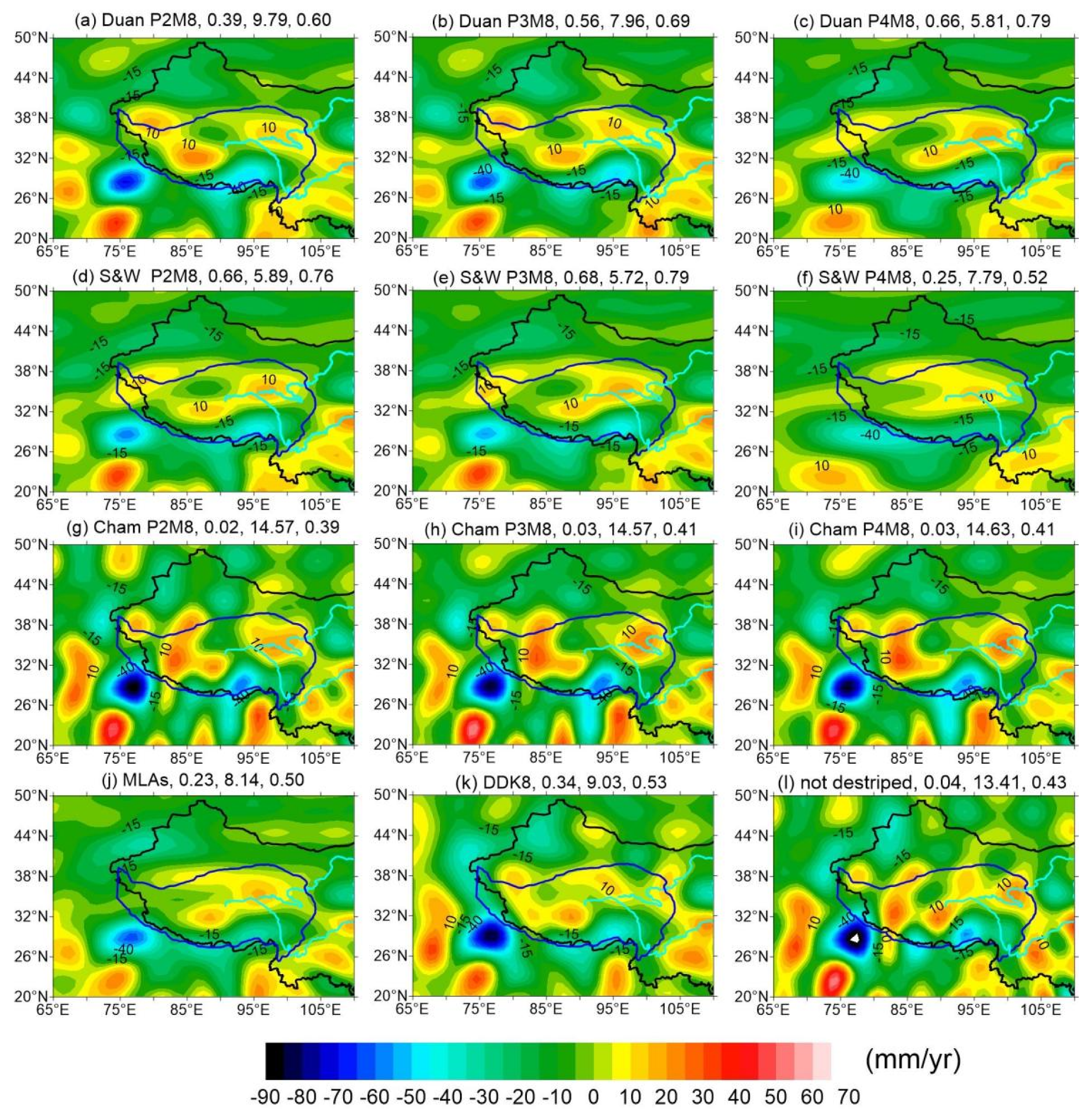
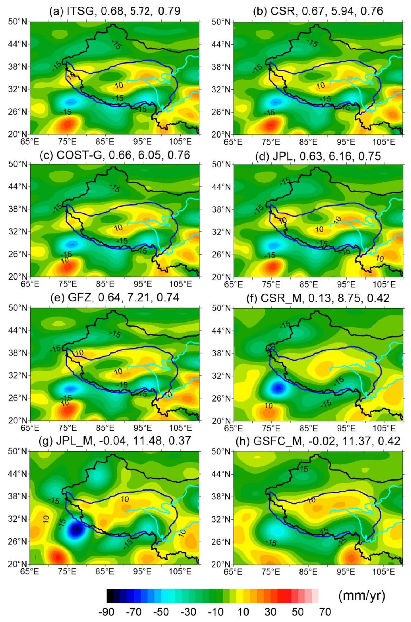
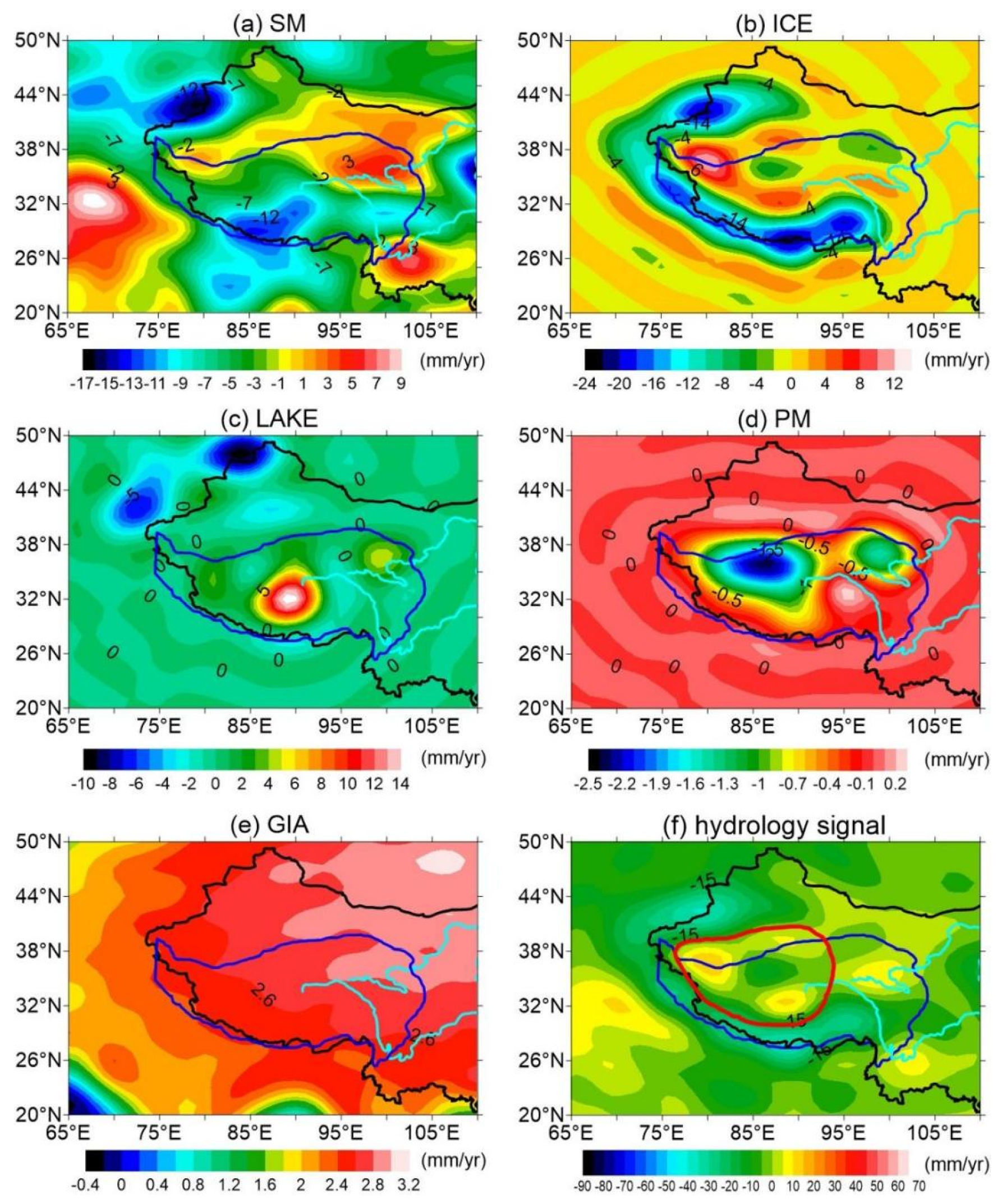

Publisher’s Note: MDPI stays neutral with regard to jurisdictional claims in published maps and institutional affiliations. |
© 2022 by the authors. Licensee MDPI, Basel, Switzerland. This article is an open access article distributed under the terms and conditions of the Creative Commons Attribution (CC BY) license (https://creativecommons.org/licenses/by/4.0/).