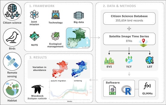
Combining Citizen Science Data and Satellite Descriptors of Ecosystem Functioning to Monitor the Abundance of a Migratory Bird during the Non-Breeding Season

Abstract

Migratory birds are particularly exposed to habitat changes in their breeding and non-breeding grounds. Remote sensing technologies offer an excellent opportunity to monitor species’ habitats from space at unprecedented spatiotemporal scales. We analyzed if remotely sensed ecosystem functioning attributes (EFAs) adequately predict the spatiotemporal variation of the Woodcock’s (Scolopax rusticola) relative abundance in southwest Europe, during autumn migration and wintering periods. We used data gathered from Woodcock monitoring through citizen science (N = 355,654 hunting trips) between 2009 and 2018. We computed a comprehensive set of EFAs on a weekly basis from three MODIS satellite products: enhanced vegetation index (EVI), tasseled cap transformation (TCT), and land surface temperature (LST). We developed generalized linear mixed models to explore the predictive power of EFAs on Woodcock’s abundance during the non-breeding season. Results showed that Woodcock abundance is correlated with spatiotemporal dynamics in primary productivity (measured through the EVI), water cycle dynamics (wetness component of TCT), and surface energy balance (LST) in both periods. Our findings underline the potential of combining citizen science and remote sensing data to monitor migratory birds throughout their life cycles—an issue of critical importance to ensure adequate habitat management in the non-breeding areas.

1. Introduction

In the face of rapid global environmental changes, it is increasingly important to understand the main factors affecting species’ habitats throughout their annual life cycle [1]. The status of habitats in wintering and migratory seasons becomes critical for species that spend part of the year in different regions. These species are particularly exposed to changes in conditions and resources. Several aspects of ecosystem functioning relevant for species have been severely affected by climate and land-use change over recent decades [2]. As the annual life cycle of migratory species involves movements between different locations, it becomes more complex to evaluate the influence of interannual environmental changes in these species [3,4]. Managers and decision makers need to be updated with the best information available on the status of both breeding and non-breeding populations to protect them effectively.

Advances in geographic information systems (GIS) and remote sensing for Earth observation have significatively improved our ability to understand, monitor, and forecast species distribution changes over recent decades [5,6]. Combining both technologies provides a broad spectrum of environmental data at unprecedented spatiotemporal scales offering increasing amounts of information about the entire planet [7,8,9]. In addition, ecological modeling has also received greater attention in recent years due to its wide range of applications for the study and conservation of biodiversity [5,10]. Species distribution models (SDMs), based on the assessment of species’ ecological niches, link georeferenced observations of a biotic response variable such as the occurrence or abundance of species with several environmental predictors through a wide range of statistical or machine learning algorithms. These techniques are powerful tools for conservation biology, allowing predictions of habitat suitability and the probability of species occurrence with relatively high accuracy [11] even when complete information of their entire distributional range is not available [6,12]. Therefore, SDMs are very useful to fill knowledge gaps about the geographic distribution of species. SDMs have been used to identify priority areas for conservation, assess environmental impacts, and predict future environmental changes, making it possible to manage critical resources or conditions that affect species habitat [8,13]. Additionally, species abundance models (SAMs) can provide critical information for species monitoring and conservation management. However, these models have received less attention from the scientific community, possibly due to difficulties in obtaining abundance data related to sampling protocols’ costs and specificity [14]. In general, species occurrence data are more accessible than population abundance data because they only require recording the presence or evidence of at least one individual rather than estimates of the absolute or relative number of individuals [15]. However, SAMs have the advantage of being much more informative and capable of providing relevant information on the distribution of species and the size of populations, which can reflect the role of essential demographic and environmental factors [15,16,17].

A major challenge in developing SDMs and SAMs relates to the choice of environmental variables. Predictor variables should match the spatial resolution of the species data to capture habitat characteristics at finer scales, thus including a wider range of information that is ecologically relevant for the species [12,18,19]. Environmental predictor variables derived from remote sensing data are commonly used to model species distributions. However, satellite images have been used mainly in conservation biology to classify, describe, and map vegetation and habitats’ structure [20]. A recent review points out that SDMs and SAMs have suffered from the lack of spatially explicit predictor variables capturing the species’ habitats dynamics throughout their annual life cycle [21]. Nevertheless, emerging remote sensing technologies face these challenges and contribute to a new generation of distribution and abundance models [13,17]. New satellite products can improve SDMs’ and SAMs’ performance by providing essential information to predict species ranges.

An example of such satellite products is the ecosystem functioning attributes (EFAs), which are biophysical descriptors of ecosystem functioning that describe exchanges of matter and energy between the biota and the environment [12,22]. EFAs are calculated from satellite recorded time series and offer a more integrated and faster assessment of ecosystem responses to environmental factors and changes than macroclimatic databases or structural attributes (e.g., vegetation height and density, landscape composition, or spatial configuration) [23]. Additionally, since EFAs are remotely detected in a standardized and synoptical fashion, species habitats’ spatial and temporal (seasonal and interannual) variability can be easily included in SAM or SDM workflows [22]. Despite these advances, they are still relatively unexplored for these purposes [13,24]. The possibility of including predictors of the seasonal and interannual habitat dynamics in SAMs can be an opportunity for studying migratory species whose annual life cycle develops in different areas of the globe with specific phenological events marking their departure, arrival, or permanence periods.

The Woodcock (Scolopax rusticola) is a migrant wader (Charadriiformes), distinguished from other scolopacids by its association with forest areas [25,26]. Environmental conditions influence the Woodcock’s behavior, especially in the non-reproductive period (i.e., wintering period), when the distribution and abundance of its populations seem to be particularly affected by temperature and rainfall [27,28,29]. The Woodcock is sensitive to the thermal regime [27,29,30] and seasonal variations in soil moisture [31,32], as well as habitat features related to vegetation cover [33,34,35]. Landscape and forest habitats’ heterogeneity can significantly affect Woodcock abundance since habitat requirements appear to vary with different stages of its annual life cycle [35]. The Woodcock’s distribution is also strongly conditioned by food availability [31,36]. It has a diet specialized in soil microfauna: arthropods, annelids (mainly worms), and slugs [36]. Low temperatures decrease its capacity to regulate body temperature and affect food accessibility since frozen water makes it harder to penetrate deeper into the soil to access the worms [37]. Under these conditions, the Woodcock shows a more irregular distribution and variable density, with stochastic events shaping its population dynamics [27]. When rainfall is strong, and the temperature is mild, food is more abundant, and the Woodcock distributes more evenly in relatively low densities.

The Woodcock is a species with great game interest in Europe, where it is estimated that 3 to 4 million individuals are hunted annually [38]. There, Woodcock hunter associations from different European countries seek to involve their affiliates in managing and conserving the species, encouraging them to collect data from their activity. Thus, a large volume of long-term data has been collected during the hunting season across Europe. This citizen science data source offers an excellent opportunity to study the factors affecting the Woodcock’s distribution and abundance during the winter season across a wide geographic area. As referred by Runge et al. [39], management and conservation actions for migratory birds need to be coordinated across different regions, habitat types, seasons, and jurisdictions. Additionally, there is an increasing consensus on the need for sustainable hunting, which depends on a deeper understanding of the factors driving the game species’ interannual population fluctuations [40].

The present study aims to understand better how ecosystem functioning influences the population abundance of migratory birds throughout the non-breeding season. To do so, we focused on the Woodcock population across southwestern Europe (Portugal, Spain, and France) during the autumn and winter seasons (migrating and wintering birds), using hunting data.

We hypothesized that remotely sensed variables depicting several dimensions of ecosystem functioning (i.e., EFAs expressing vegetation and edaphoclimatic conditions) and their seasonal dynamics could explain the spatiotemporal variation of the Woodcock’s abundance. In particular, we took advantage of a long-term time series obtained from citizen science (N = 355,654 hunting trips) gathered between 2009 and 2018. We computed a comprehensive set of zonal statistical parameters for three EFAs, for 8-day periods, from MODIS satellite products: enhanced vegetation index (EVI), tasseled cap transformation (TCT), and land surface temperature (LST). Finally, we analyzed to what extent these remotely sensed indicators of primary productivity, water, and energy balance predict the Woodcock’s abundance and whether this effect varies between autumn migration and wintering seasons.

2. Materials and Methods

2.1. The Woodcock

The Woodcock has a wide distribution in the Palearctic region (Figure 1) [25,38]. It is essentially a migrant, except for some resident or short-distance migrant populations, in the archipelagos of the Canaries, Madeira, and the Azores, and in some maritime countries in southwest Europe and the British Isles [41,42]. In the Western Palearctic, it reproduces mainly in central, northern, and eastern Europe and Russia, and winters in central and southeast Europe, particularly in France and the Iberian Peninsula [25,43].

During the breeding season, the Woodcock selects habitat mosaics with specific characteristics such as deciduous forest habitats [46,47], mixed forest, or conifers [25,48,49]. During the wintering period, it shows less specific habitat requirements, selecting different habitats such as hedged forests during the day, for refuge, and meadows at night, for feeding [25,31,50], where it can find high invertebrate biomass, particularly annelids [26,51].

The current Woodcock breeding population in the Western Palearctic is estimated to be between 10 and 26 million individuals, most of which spend the winter in western and southern Europe and northern Africa [52,53]. However, these estimates are mainly supported by specialists’ opinions and not on objective data collected in the field [54]. The Woodcock is a solitary, elusive, and cryptic species, limiting classic survey techniques usually applied to assess bird abundance [34,35,55,56]. Thus, citizen science data obtained from hunting activity offer an important opportunity to study this species.

The Woodcock appears in Part A of Annex II and Part B of Annex III of the “Birds Directive”, which means it can be hunted in the geographical area where the directive is applicable. However, the effects of hunting on their populations are still poorly assessed, with evidence of an additive effect on mortality and causing the use of more extensive areas during the day [33,57]. In addition to hunting, land-use changes may also cause some disturbance in the Woodcock’s annual life cycle. Although there are some studies about its ecology, these are mainly concentrated in the breeding period and/or in restricted areas of its distribution, such as those carried out using ringing data [28], stable isotopes [43], and telemetry [49,58].

Its current global conservation status is evaluated as Least Concern; the only available regional trend assessment concerns Europe, where the population seems to be stable [59].

2.2. Study Area and Hunting Data

The study area covers central and southwestern Europe (France, Spain, and Portugal), which represents one of the main wintering areas for Woodcock [25,43] (see Figure 1). Due to the long hunting traditions, population monitoring programs were developed to support a more sustainable hunting activity in these countries. In Europe, Woodcock hunter associations from different countries are gathered in the Federation of Western Palearctic Woodcock Hunter Association (Féderation des Associations Nationales des Bécassiers du Palearctique Occidental (FANBPO)), which facilitates their cooperation and communication.

We analyzed data collected between 2009 and 2018 by Woodcock hunters, members of the Club National des Bécassiers, the Club de Cazadores de Becada, and the Associação Nacional de Caçadores de Galinholas, during Woodcock hunting trips in mainland France, Spain, and Portugal, respectively (Figure 1). Woodcock hunting seasons occur from September to February of the following year, with differences in the beginning date between these countries (France: 14 September; Spain: 8 October; Portugal: 1 November), and in the number of hunting days and bag limits. Only data collected from hunting with pointing dogs were considered in the analyses. Hunters registered the date, location, duration, and number of Woodcocks seen for each hunting trip.

A total of 355,654 hunting trip records were analyzed: 326,519 (~92%) from France, 25,746 (~7%) from Spain, and 3389 (~1%) from Portugal (Figure 1), totaling 536,873 contacts with Woodcock during 1,154,222 h of hunting. We estimated a relative abundance index corresponding to the number of different Woodcock observed per hour in each hunting trip (ICA or ICA1 [60,61,62]). This abundance index is strongly related to another relative abundance index obtained from night ringing sessions (IAN or NIA) and is considered a good indicator to evaluate winter abundance variation [60,61,62].

Since the location of the hunting trips was provided with variable detail among the three countries, the relative abundance index values were aggregated at level 3 of NUTS classification (NUTS-III), which corresponds to departments in France, provinces in Spain, and intermunicipal entities in Portugal. The average area (±standard deviation) of these units is 6320.4 ± 8054.7 km², 8576 ± 5698.6 km², and 3676 ± 2020.7 km², for France (n = 88), Spain (n = 41), and Portugal (n = 23), respectively.

2.3. Remote Sensed Ecosystem Functioning Variables

To evaluate how ecosystem functioning influences the Woodcock’s relative abundance, we computed a comprehensive set of zonal statistical parameters for three ecosystem functioning attributes from MODIS satellite data products: enhanced vegetation index (EVI), tasseled cap transformation (TCT), and land surface temperature (LST) [63,64] (

Table 1. List of variables estimated from the Terra/MODIS satellite imaging products. For the list of acronyms of the remote sensed ecosystem functioning variables, see Table A3.

Components of Ecosystem Functioning	Ecosystem Functioning Attributes—EFAs	MODIS Product(s)/Pixel Size and Time Frequency	Zonal Statistical Parameters (NUTS-III)
Carbon cycle (primary productivity)	EVI—Enhanced vegetation index	MOD09A1 (v006)—Surface reflectance 500 m (8-day composite)	Minimum (min.) Average (avg.) Maximum (max.) Range (range)
Water cycle (water in soil/vegetation)	TCTwet—Tasseled cap transformation—water component
Energy balance	LST—Land surface temperature	MOD11A2 (v006)—Surface temperature and emissivity 1000 m (8-day composite)

). These variables are suited to characterizing ecosystem functioning in a repeatable, continuous, and standardized way, being related to primary productivity, water, and energy balance [12,17,22].

EVI (1) is an optimized vegetation index with improved sensitivity in high biomass regions and can reduce atmospheric contamination [65]. The EVI was calculated using the blue, red, and near-infrared (NIR) bands with the following parameters: L = 1, C1 = 6, C2 = 7.5, and G (gain factor) = 2.5.

$$\mathrm{G}\times \frac{\left(\mathrm{NIR}-\mathrm{RED}\right)}{\left(\mathrm{NIR}+\mathrm{C}1\times \mathrm{RED}-\mathrm{C}2\times \mathrm{Blue}+\mathrm{L}\right)}$$

(1)

EVI value can vary between −1 and 1, with the lowest values being associated with artificial cover types and the highest values, closer to one, are related to higher levels of biomass, vegetation cover, leaf area index, or photosynthetic activity. The EVI was obtained from the MODIS MOD13Q1 product with 250 m spatial resolution and 8-day temporal resolution.

TCT allows, similarly to principal component analysis, performance of a linear transformation to satellite spectral data to highlight specific aspects of the land surface. These components are related to “brightness” (which approximately translates to the albedo coefficient), “greenness” (as a proxy of vegetation biomass), or the “wetness” component (as a proxy of water content in the soil and vegetation). The coefficients used in the transformation to the wetness component were derived from Zhang et al. [66] (

Table A1. Coefficients used in the tasseled cap transformation (TCT) of MODIS NBAR products (derived from [66]). In bold, the TCT Wetness (TCTwet) component used for the analyses.

Band	Red	Near-IR	Blue	Green	M-IR	M-IR	M-IR
MODIS band wavelength (nm)	620–670	841–876	459–479	545–565	1230–1250	1628–1652	2105–2155
Brightness	0.3956	0.4718	0.3354	0.3834	0.3946	0.3434	0.2964
Greenness	−0.3399	0.5952	−0.2129	−0.2222	0.4617	−0.1037	−0.4600
Wetness	0.1084	0.0912	0.5065	0.4040	−0.2410	−0.4658	−0.5306
Fourth	0.4527	0.4480	−0.3869	−0.1277	−0.3164	−0.4993	0.2829
Fifth	0.6478	−0.2448	−0.3705	0.0068	0.1385	0.2564	−0.5461
Sixth	−0.2332	0.3348	−0.2764	0.3516	−0.5986	0.5032	−0.1515
Seventh	−0.1930	−0.2052	−0.4725	0.7049	0.3107	−0.2935	0.1334

). The TCTwet index (i.e., TCT transformation for the wetness component) value can vary between −1 and 1 and indicates, in a relative way, the amount of water in the soil or vegetation, being able to, under continuous observation, show the availability and water balance in a given region. TCTwet was calculated from the MODIS MOD09A1 product with 500 m spatial resolution and 8-day temporal resolution.

To calculate LST from the MODIS product MOD11A2 (with 1 km spatial resolution and 8-day temporal resolution), a multiplicative conversion factor of 0.02 (units in Kelvin) was applied.

Using metadata of MODIS images, the pixels marked as clouds were removed to avoid spurious values. The data collection was carried out through original images for each variable (Table 1) and by applying zonal statistics (i.e., aggregating all the pixels included in a given area) for each NUTS-III region (see the available list in

Table A2. List of NUTS-III and the respective number of journeys.

Country	NUTS-III	Designation	N° of Journeys
Portugal	PT111	Alto Minho	1342
Portugal	PT112	Cávado	63
Portugal	PT119	Ave	39
Portugal	PT11A	Área Metropolitana do Porto	20
Portugal	PT11B	Alto Tâmega	319
Portugal	PT11C	Tâmega e Sousa	10
Portugal	PT11D	Douro	71
Portugal	PT11E	Terras de Trás-os-Montes	11
Portugal	PT150	Algarve	10
Portugal	PT16B	Oeste	61
Portugal	PT16D	Região de Aveiro	82
Portugal	PT16E	Região de Coimbra	119
Portugal	PT16F	Região de Leiria	72
Portugal	PT16G	Viseu Dão-Lafões	32
Portugal	PT16H	Beira Baixa	17
Portugal	PT16I	Médio Tejo	201
Portugal	PT16J	Beiras e Serra da Estrela	15
Portugal	PT170	Área Metropolitana de Lisboa	53
Portugal	PT181	Alentejo Litoral	67
Portugal	PT184	Baixo Alentejo	45
Portugal	PT185	Lezíria do Tejo	51
Portugal	PT186	Alto Alentejo	115
Portugal	PT187	Alentejo Central	574
Spain	ES111	A Coruña	320
Spain	ES112	Lugo	551
Spain	ES113	Ourense	11
Spain	ES114	Pontevedra	430
Spain	ES120	Asturias	1082
Spain	ES130	Cantabria	4065
Spain	ES211	Álava/Araba	2337
Spain	ES212	Guipúzcoa/Gipuzkoa	814
Spain	ES213	Vizcaya/Bizkaia	1228
Spain	ES220	Navarre	2786
Spain	ES230	La Rioja	23
Spain	ES241	Huesca	392
Spain	ES242	Teruel	173
Spain	ES243	Zaragoza	264
Spain	ES300	Madrid	101
Spain	ES411	Ávila	20
Spain	ES412	Burgos	2543
Spain	ES413	León	983
Spain	ES414	Palencia	859
Spain	ES415	Salamanca	295
Spain	ES416	Segovia	26
Spain	ES417	Soria	428
Spain	ES418	Valladolid	101
Spain	ES419	Zamora	91
Spain	ES423	Cuenca	1
Spain	ES424	Guadalajara	65
Spain	ES425	Toledo	21
Spain	ES431	Badajoz	2
Spain	ES432	Cáceres	11
Spain	ES511	Barcelona	2782
Spain	ES512	Girona	2099
Spain	ES513	Lleida	289
Spain	ES514	Tarragona	82
Spain	ES521	Alicante	63
Spain	ES522	Castellón/Castelló	93
Spain	ES612	Cádiz	20
Spain	ES614	Granada	1
Spain	ES615	Huelva	61
Spain	ES616	Jaén	1
Spain	ES617	Málaga	159
Spain	ES620	Murcia	73
France	FR102	Seine-et-Marne	66
France	FR103	Yvelines	23
France	FR104	Essonne	79
France	FR108	Val-d’Oise	10
France	FRB01	Cher	1641
France	FRB02	Eure-et-Loir	596
France	FRB03	Indre	1913
France	FRB04	Indre-et-Loire	2213
France	FRB05	Loir-et-Cher	437
France	FRB06	Loiret	435
France	FRC11	Côte-d’Or	1512
France	FRC12	Nièvre	1592
France	FRC13	Saône-et-Loire	1608
France	FRC14	Yonne	553
France	FRC21	Doubs	3514
France	FRC22	Jura	5954
France	FRC23	Haute-Saône	3437
France	FRC24	Territoire de Belfort	139
France	FRD11	Calvados	700
France	FRD12	Manche	3203
France	FRD13	Orne	703
France	FRD21	Eure	403
France	FRD22	Seine-Maritime	248
France	FRE11	Nord	90
France	FRE12	Pas-de-Calais	1361
France	FRE21	Aisne	350
France	FRE22	Oise	478
France	FRE23	Somme	377
France	FRF12	Haut-Rhin	2
France	FRF21	Ardennes	174
France	FRF22	Aube	158
France	FRF23	Marne	25
France	FRF24	Haute-Marne	675
France	FRF31	Meurthe-et-Moselle	4
France	FRF33	Moselle	25
France	FRF34	Vosges	6
France	FRG01	Loire-Atlantique	1116
France	FRG02	Maine-et-Loire	3148
France	FRG03	Mayenne	745
France	FRG04	Sarthe	1156
France	FRG05	Vendée	2640
France	FRH01	Côtes-d’Armor	6553
France	FRH02	Finistère	5842
France	FRH03	Ille-et-Vilaine	1421
France	FRH04	Morbihan	5698
France	FRI11	Dordogne	13,413
France	FRI12	Gironde	15,319
France	FRI13	Landes	19,028
France	FRI14	Lot-et-Garonne	3640
France	FRI15	Pyrénées-Atlantiques	11,162
France	FRI21	Corrèze	9949
France	FRI22	Creuse	5263
France	FRI23	Haute-Vienne	7420
France	FRI31	Charente	6615
France	FRI32	Charente-Maritime	18,732
France	FRI33	Deux-Sèvres	1687
France	FRI34	Vienne	4161
France	FRJ11	Aude	2166
France	FRJ12	Gard	12,795
France	FRJ13	Hérault	10,565
France	FRJ14	Lozère	4667
France	FRJ15	Pyrénées-Orientales	2030
France	FRJ21	Ariège	3181
France	FRJ22	Aveyron	3804
France	FRJ23	Haute-Garonne	2385
France	FRJ24	Gers	5468
France	FRJ25	Lot	8634
France	FRJ26	Hautes-Pyrénées	3786
France	FRJ27	Tarn	4454
France	FRJ28	Tarn-et-Garonne	5205
France	FRK11	Allier	1424
France	FRK12	Cantal	1923
France	FRK13	Haute-Loire	5946
France	FRK14	Puy-de-Dôme	5035
France	FRK21	Ain	2024
France	FRK22	Ardèche	6359
France	FRK23	Drôme	13,397
France	FRK24	Isère	8457
France	FRK25	Loire	2115
France	FRK26	Rhône	562
France	FRK27	Savoie	3556
France	FRK28	Haute-Savoie	1595
France	FRL01	Alpes-de-Haute-Provence	6768
France	FRL02	Hautes-Alpes	556
France	FRL03	Alpes-Maritimes	3906
France	FRL04	Bouches-du-Rhône	4159
France	FRL05	Var	7229
France	FRL06	Vaucluse	2956

in the Appendix A). Given the large size of the spatial units (NUTS-III), in addition to the average value for each unit, we also computed the minimum and the maximum value (Table 1) to characterize the extreme conditions at the NUTS level. We also calculated each variable’s range to characterize the spatial heterogeneity inside each NUTS-III region (the larger the range, the greater the heterogeneity within the NUTS-III region). Thus, four zonal statistic measures were used to characterize the data distribution at the NUTS level: minimum, average, maximum, and range. These values were estimated for 8-day periods from daily images extracted between September and February of the following year, covering the annual hunting seasons from 2009 (September) to 2018 (February). The EVI values at the NUTS-III level changes with the latitude and 8-day period. All image reprocessing and calculation processes were performed in the Google Earth Engine cloud-based platform [67]. We used “dplyr” and “tidyr” R packages [68,69] for data management and preprocessing.

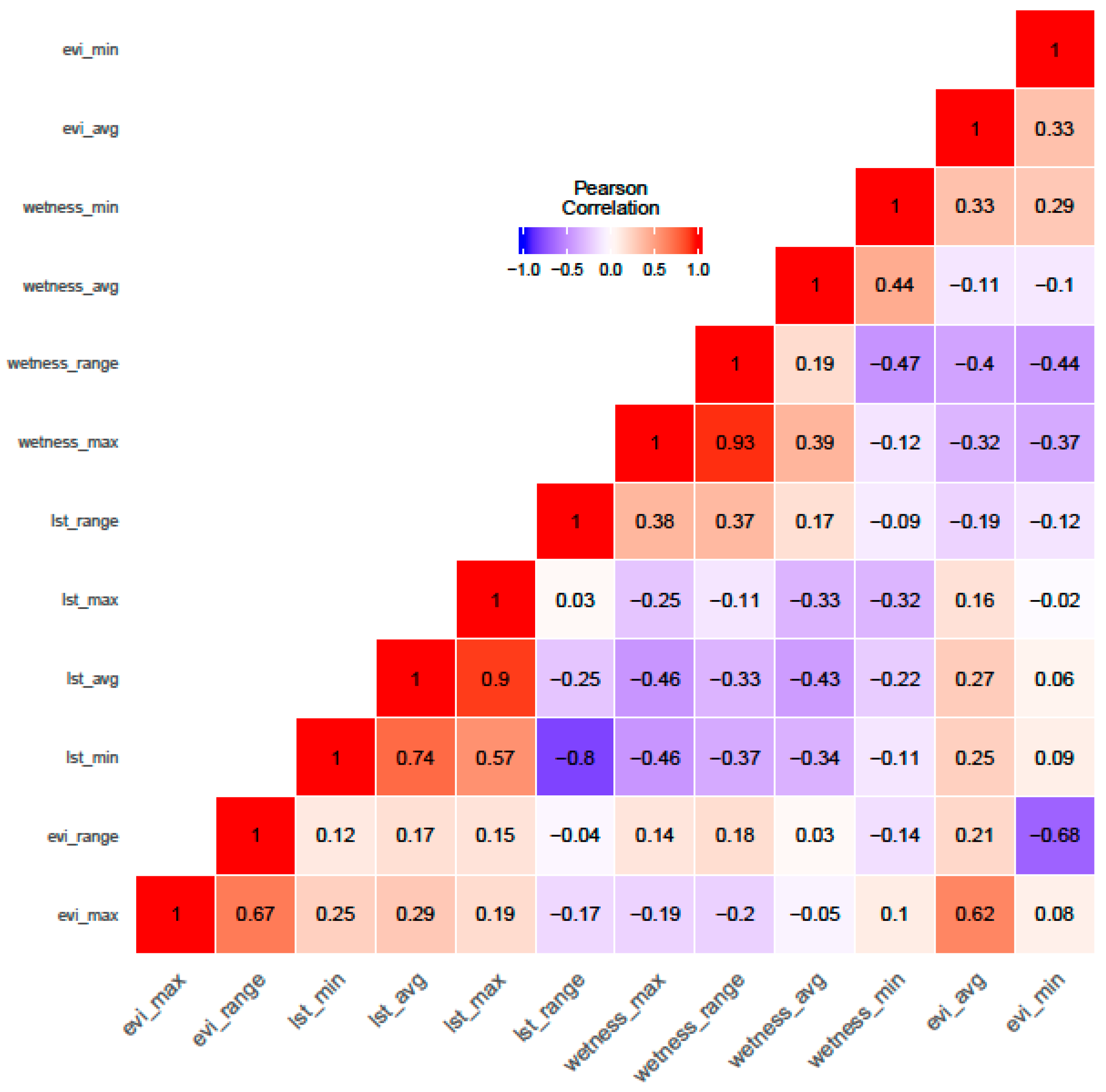
2.4. Variable Selection and Ranking

The data on the relative abundance of Woodcock were grouped by week to match as close as possible with the time scale of the available remote sensing data (Figure 2). Both data types were divided into two periods, corresponding to two phases of the species’ annual life cycle, following [54,70]:

1.

Autumnal migration, from early September (first week of the month, week 35) to mid-December (second week of the month, week 50).

2.

Wintering season, from mid-December (week 51) to late February (week 9).

All remote sensing variables were standardized (2), considering the respective mean and standard deviation values using the “scale” function available in the “arm” R package [71].

$$\frac{\mathrm{x}-\mathrm{mean}\left(\mathrm{x}\right)}{\mathrm{standard}\mathrm{deviation}\left(\mathrm{x}\right)}$$

(2)

To avoid multicollinearity problems, we calculated Pearson’s correlation coefficient between each pair of variables (see the list and respective acronyms in

Table A3. Acronyms of the remote sensed ecosystem functioning variables (defined in Table 1), by statistical measure. (*) indicates the variables used in the models after the correlation analysis.

Statistical Parameter	Index Name	Code
Minimum	EVI	evi_min
	TCTwet	wetness_min
	LST	lst_min
Average	EVI	evi_avg *
	TCTwet	wetness_avg *
	LST	lst_avg *
Maximum	EVI	evi_max *
	TCTwet	wetness_max
	LST	lst_max *
Range	EVI	evi_range *
	TCTwet	wetness_range
	LST	lst_range *

). The correlations were represented graphically (Figure A1). The variance inflation factor (VIF) was also calculated with the “usdm” R package [72] to estimate how much a regression coefficient’s variance is inflated by multicollinearity. The variables with Pearson’s correlation coefficient (with absolute value) greater than 0.7 and a VIF value greater than three were excluded from further analyses [73,74].

To explore the effects of remotely sensed ecosystem functioning variables (fixed factors) on the spatiotemporal variation of the Woodcock’s relative abundance (dependent variable), mixed generalized linear models (GLMMs) were developed separately for the migration and wintering period. To avoid outliers that could affect model inference, we removed abundance values greater than the interquartile distance multiplied by 1.5 [75,76]. The “country” and the “week” nested with the annual “hunting season” were considered as random effects to account for repeated measurements within and across units of time (“week”) and space (“countries”). Each country has a hunting period due to climatic and hunting legal specificities, so a “country” level effect must be accounted for. The “week” was also included as a random effect nested with the annual “hunting season” because abundance data have been collected every week of the migratory and wintering season over the years. Since the response variable (i.e., the relative abundance index) is a continuous variable, our models were fitted assuming a normal distribution and using the “link” identity function. Previous analyses with Poisson and negative binomial error distributions and zero-inflated models were finally ruled out due to their lower explanatory power (conditional R² value ranged between 0.07 and 0.12, and marginal R² between 0.04 and 0.07). The analyses were performed with the “glmmTMB” R package [77]. Model performance was assessed using the “check_model” function, available in the “performance” R package [78]. This complementary analysis confirms various model assumptions: normality of residuals, normality of random effects, heteroscedasticity, homogeneity of variance, and multicollinearity (see Figure A2 and Figure A3 in the Appendix A).

In addition, a multi-model inference approach was performed for both migratory and wintering seasons, running models from all possible combinations of environmental variables (predictors) to verify the importance of each one of them through the “dredge” function of the “MuMIn” R package [79]. Finally, only those models with a delta Akaike information criterion (AIC) value of less than four were considered relevant [80]. The variables were considered significant for p-values < 0.05. Šidák’s correction [81] was computed to adjust p-values for multiple comparisons.

Data graphs were created with the “ggplot2” [82], “ggpmisc” [83], and “cowplot” [84] R packages.

3. Results

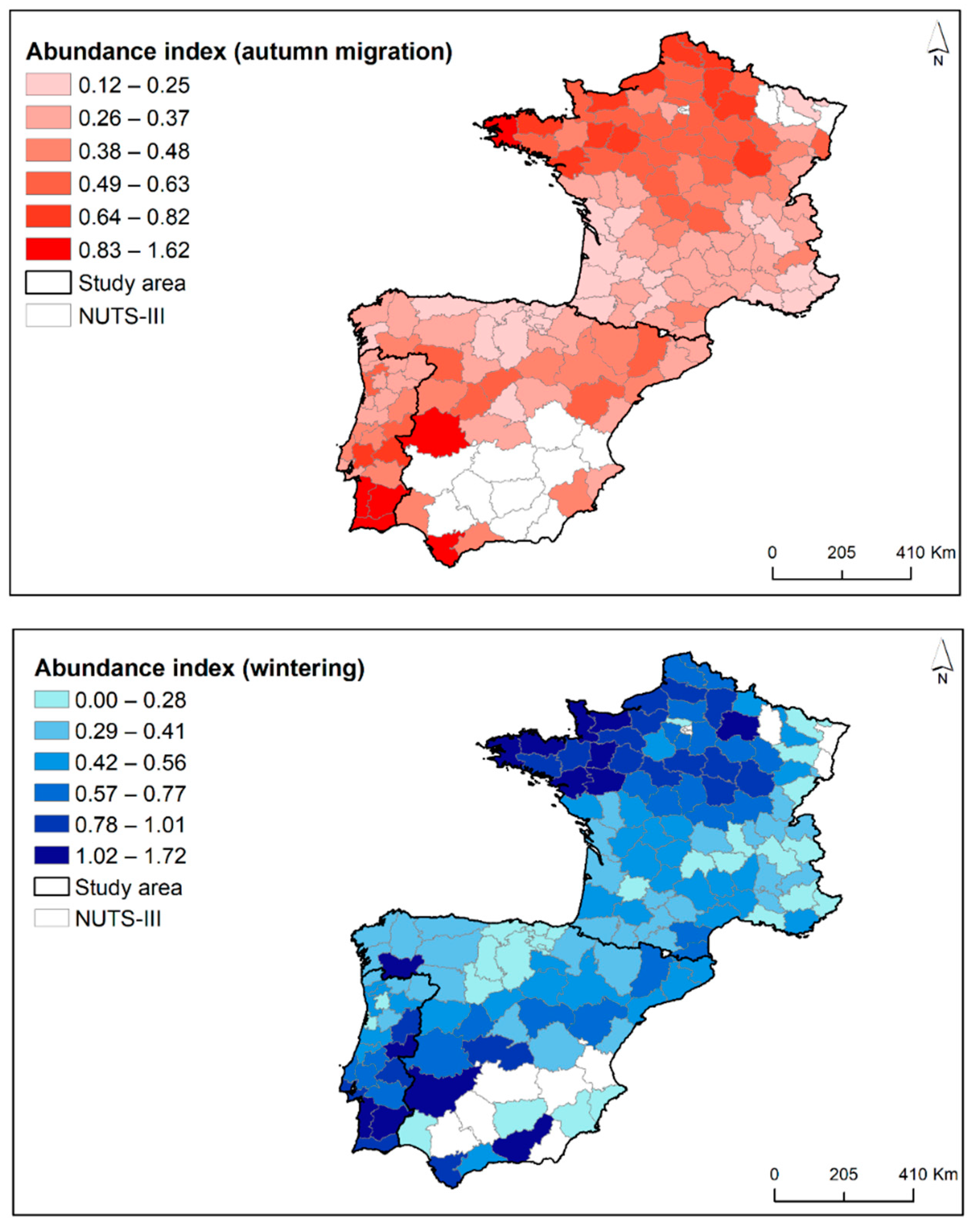
3.1. Patterns of Spatiotemporal Variation in Woodcock Abundance

Our results confirm the expected variation in the Woodcock’s relative abundance over the hunting season (Figure 3). The relative abundance index initially increases over the migration period until reaching a maximum peak, followed by a relatively stable phase that coincides with the wintering season. There is a slight time lag in this pattern between countries; initially, the abundance increases in France, Spain, and Portugal. Regarding the spatial variation of Woodcock abundance, the species is more abundant in the north of France, the southwest of Spain, and in the center and the south of Portugal, for both wintering and migration periods (Figure 4). Some sampling units have no abundance data available, particularly in southern Spain and northeastern France.

3.2. Predictors of Spatiotemporal Variation in Woodcock Abundance

3.2.1. Autumnal Migration

The GLMM fitted for the autumn migration period, including all environmental variables, presented a moderate explanatory ability, with a conditional R² value of 0.33 and a marginal R² value of 0.09. Six of the seven variables considered for analysis had a significant effect (

Table 2. Generalized linear mixed model (GLMM) results for the autumn migration and wintering periods. Estimate of regression coefficients results from an averaged model obtained from those with delta AIC < 4. The importance of each ecosystem functioning variable (last column) is represented by the number of times that each variable appears contained in the explanatory models (delta AIC < 4). EFAs: EVI—enhanced vegetation index; TCTwet—tasseled cap transformation—water component; LST—land surface temperature; respective maximum (max), minimum (min), average (avg), and range (range) values. Šidák’s correction [81] was computed to adjust p-values for multiple comparisons. Significant results, at p < 0.05, are shown in bold and underlined if significant after correction for seven comparisons.

Variable	Autumn Migration					Wintering
	Estimate	Error	Z Value	Probability (>|z|)	Number of Models Contained	Estimate	Error	Z Value	Probability (>|z|)	Number of Models Contained
evi_range	0.072	0.008	9.541	<0.001	2	0.069	0.009	7.723	<0.001	4
evi_max	−0.104	0.010	−10.512	<0.001	2	−0.107	0.010	−10.774	<0.001	4
evi_avg	0.073	0.008	8.982	<0.001	2	0.128	0.011	11.692	<0.001	4
lst_range	−0.010	0.008	−1.138	0.255	1	0.014	0.001	1.350	0.177	2
lst_max	0.044	0.009	4.659	<0.001	2	0.056	0.011	5.130	<0.001	4
lst_avg	−0.209	0.015	−13.766	<0.001	2	−0.095	0.018	−5.277	<0.001	4
wetness_avg	−0.080	0.010	−8.220	<0.001	2	−0.021	0.010	−2.129	0.0333	2

). Those with the most significant effect were the medium LST (Z = −13.766; p < 0.001) and the maximum EVI (Z = −10.512; p < 0.001), both with a negative effect on species abundance (Table 2). The EVI amplitude and medium value (Z = 9.541; p < 0.001; Z = 8.982; p < 0.001) also stand out, having a positive effect on abundance. The medium value of the TCTwet component also had a significant and negative effect on the abundance of the species (Z = −8.220; p < 0.001) and the maximum LST had a positive effect (Z = 4.659; p < 0.001). All these significant variables are present in all models considered relevant in AIC multimodel inference (i.e., delta AIC < 4; Table 2). LST amplitude was the only descriptor of ecosystem functioning that was not significant (p = 0.225; Table 2).

3.2.2. Wintering

The GLMM built for the wintering period, including all environmental variables, also presented a moderate explanatory capacity, with a conditional R² value of 0.16 and a marginal R² value of 0.09. Five of the seven variables considered for analysis had a significant effect (Table 2). Those with the most significant effect were the average EVI (Z = 11.692; p < 0.001) and the maximum EVI (Z = −10.774; p < 0.001), the first with a positive effect and the second with a negative effect on the species abundance (Table 2). EVI amplitude (Z = 7.723; p < 0.001) showed a positive effect, while the average and maximum value of the LST (Z = −5.277; p < 0.001; Z = 5.130; p < 0.001, respectively) had for the first a negative effect and the second a positive effect. The maximum LST component positively affected the species relative abundance (Z = 5.130; p < 0.001). These variables are shown in all the models considered, supported by AIC-based multimodel inference (delta AIC < 4; Table 2). The average value of the TCTwet component (Z = −2.129; p = 0.333) and the amplitude of LST (Z = 1.350; p = 0.177; Table 2) are the only descriptors of ecosystem functioning that were not significant after adjustment for multiple comparisons.

4. Discussion

4.1. Ecosystem Functioning Attributes and Woodcock Abundance

Our results confirm that remotely sensed habitat descriptors (namely EFAs and their seasonal dynamics) have a significant explicative ability for the spatiotemporal patterns of abundance of migratory birds. In the autumn migration period, the maximum EVI and average LST (descriptors of primary productivity and energy balance, respectively) correlated significantly and negatively with Woodcock abundance. The maximum EVI stands out in the wintering period and the average EVI has a positive effect. Additionally, significantly correlated, in both periods, are the EVI amplitude values.

The highest maximum EVI values signal those areas with the highest primary productivity [65], such as forest areas with dense vegetation. These characteristics seem to be associated with the Woodcock’s lower abundance in the two studied periods (Table 2). This result is consistent with previous knowledge about the species’ habitat requirements indicating a preference for mixed areas of forests and hedges during the day and fields and meadows at night, rather than areas of homogeneous and dense forest [31,33,49]. On the other hand, higher EVI amplitude values indicate a greater heterogeneity in the vegetation cover. This situation will benefit the Woodcock, which, in these periods of its annual life cycle, needs open areas for night feeding (i.e., pastures, natural or artificial meadows, agricultural fields) and forest and bush areas for shelter during the day [31,33,49]. Our results are aligned with recent studies that support a relationship between primary productivity and the migration of long-distance migratory birds, pointing out that their migratory movement is influenced by seasonal changes in the landscape’s resource availability [86].

The maximum value of land surface temperature (LST) showed a significant and positive correlation with abundance but was slightly higher in the wintering period (Table 2). The average value of LST is negatively related to Woodcock abundance. This effect may indicate that the maximum temperature at the surface (reached during the day) is important. These low temperatures imply a greater difficulty for birds regarding body temperature regulation with subsequent increases in energy requirements and, therefore, food intake [30]. Péron et al. [37] demonstrated that Woodcock make great movements in winter conditioned by the air temperature. On the other hand, it is also known that the low temperatures reached during the wintering period hamper accessibility to their primary food source, earthworms, obtained by probing the soil [37]. Thus, the maximum value of the temperature at the surface, reached during the daytime, can allow favorable conditions for accessing food, at least in a certain period of the day. Finally, LST amplitude does not seem to influence Woodcock abundance in both periods significantly. Our results reinforce the interest in satellite products of surface temperature, more related to the conditions experienced by individuals on the ground in critical periods of their life cycle [87].

The average value of the TCT wetness component (TCwet; a descriptor of the water cycle in the soil/vegetation) made a significant contribution, negatively affecting the species’ abundance in the migration period (Table 2). This result may indicate that this species avoids areas with high levels of waterlogging (flooding), detrimental to obtaining food. The Woodcock, unlike other waders highly dependent on water dynamics such as the Common Snipe (Gallinago gallinago) [88], is not frequently seen in habitats with these characteristics, such as peat bogs and swamps [25].

4.2. Advantages, Limitations, and Future Perspectives

Currently, most studies indicate that habitat loss and degradation (such as the degradation and fragmentation of forest mosaics or the intensification of agricultural practices) and climate change are significant threats to species and ecosystems [89,90]. For birds, climate change influences their phenology, population dynamics, abundance, and distribution [91,92,93].

However, although these changes affect bird communities, it is unclear which factors are most prevalent in each case and which pathways. Different factors are challenging to analyze independently. Ecosystem functioning attributes (EFAs) are multipurpose descriptors that offer a more integrative and rapid assessment of responses to environmental changes. Our results allow us to verify that the abundance of Woodcock in autumn migration and winter periods is affected by several dimensions linked to primary productivity dynamics, the water cycle (water in the soil and vegetation), and ecosystems’ energy balance. These results are consistent with those obtained in previous studies, highlighting the validity of these remotely sensed indicators for species distribution and abundance assessments [12,17,22,23,88,94,95]. Several studies have already demonstrated the advantages of using models calibrated with functional variables over those based on models calibrated with exclusively climatic variables since the former allowed for capture of the joint effect of changes in climate and land cover/use on the availability of habitat for a broad group of threatened species [22,95]. Other studies about the variation in threatened plant species abundance and various bird species (especially for migrant, forest specialist species) also confirmed a greater predictive power of models calibrated with functional variables related to productivity and energy balance compared to models based on macroclimatic data or landscape composition variables [17,95].

Migratory bird species, especially those considered for hunting, such as the Woodcock, represent a greater challenge for management and conservation policies. It is vital to consider territorial continuity (beyond administrative countries’ boundaries) to analyze which factors affect species and an adequate definition of population management goals. In this sense, our study considered a broader and more representative area of the distribution in autumn migration and wintering of Woodcock than previous studies (e.g., [31,96]).

The use of data collected from hunting activity to study game species’ population dynamics is often hampered by the temporal (between hunting seasons) and the spatial variation in their quantity and quality [96,97,98,99]. The data collected often do not include metadata that allow quantifying the hunting effort (e.g., time dedicated to hunting on each journey or the area covered). Our relative abundance index considers an effort variable (sampling effort, i.e., the time spent hunting). In addition, it reports the number of birds seen and not the number of birds hunted, which reduces the influence of certain factors such as legal limitations due to the catch limits in each country. Thus, previous works have recognized this index as a useful tool [60,61,62].

On the other hand, hunting data present some limitations that must be considered. NUTS-III regions were chosen due to the location of the hunting trips that were provided with variable detail among the three countries. The large size of the NUTS-III regions leads to high environmental heterogeneity within and among them. Being aware of this limitation, we think that this dataset still provides vital information since it consists of more than 350,000 records, collected over a long time interval (nine hunting seasons) and a large geographical extent.

Still, the spatial resolution used for analyses prevents a more refined characterization of the species habitat and its ecological requirements, partly explaining the low values of marginal R². An increase in the spatial resolution at which the abundance data are collected will improve future studies since alternative satellites such as Landsat or Sentinel (e.g., [100]) would allow calculating EFAs at a finer spatial resolution (up to 30 m and 10 m, respectively) although with less temporal resolution than MODIS. In addition, the application of predictive modeling techniques based on artificial intelligence such as machine learning algorithms (e.g., random forest or artificial neural networks) can also improve our ability to predict the species’ abundance from space.

4.3. Final Considerations

The European Union (EU) seeks to curb biodiversity loss, a task that needs updated knowledge of the general conservation status of species (including wild birds) and habitats of community interest under the 1992 “Habitats Directive” (92/43/EEC) and the 1979 “Birds Directive” (2009/147/EC). However, the information on birds is still considered insufficient, as is the case in Iberian territory [10].

The present work used a new explanatory analysis for assessing the variation of Woodcock abundance in autumn and winter at large spatial and temporal scales, based on ecosystem functioning attributes obtained by Earth observation satellites. Additionally, it demonstrates the importance of citizen science programs in collecting data essential for monitoring biodiversity.

The approach developed can be applied to other taxa since it establishes strong relationships between the species abundance and essential ecosystem functions and vital ecological processes closely related to the water and carbon cycles and the energy balance. Considering the increasing availability of remote sensing products, these data provide a promising opportunity for integrating ecosystem dynamics into habitat monitoring to support management and species conservation policies. This is especially relevant given the current context of global environmental changes and the new environmental, agricultural, and nature restoration policies to be implemented in Europe in the coming decades in areas critically important for Woodcock.

References

1. Bairlein, F. Migratory birds under threat. Science 2016, 354, 547–548. [Google Scholar] [CrossRef] [PubMed]
2. Pecl, G.T.; Araújo, M.B.; Bell, J.D.; Blanchard, J.; Bonebrake, T.C.; Chen, I.-C.; Clark, T.D.; Colwell, R.K.; Danielsen, F.; Evengård, B.; et al. Biodiversity redistribution under climate change: Impacts on ecosystems and human well-being. Science 2017, 355, eaai9214. [Google Scholar] [CrossRef] [PubMed]
3. Easterling, D.R.; Meehl, G.A.; Parmesan, C.; Changnon, S.A.; Karl, T.R.; Mearns, L.O. Climate extremes: Observations, modeling, and impacts. Science 2000, 289, 2068–2074. [Google Scholar] [CrossRef] [PubMed] [Green Version]
4. Walther, G.-R.; Post, E.; Convey, P.; Menzel, A.; Parmesan, C.; Beebee, T.J.; Fromentin, J.-M.; Hoegh-Guldberg, O.; Bairlein, F. Ecological responses to recent climate change. Nature 2002, 416, 389–395. [Google Scholar] [CrossRef] [PubMed]
5. Guisan, A.; Tingley, R.; Baumgartner, J.B.; Naujokaitis-Lewis, I.; Sutcliffe, P.R.; Tulloch, A.I.; Regan, T.J.; Brotons, L.; McDonald-Madden, E.; Mantyka-Pringle, C. Predicting species distributions for conservation decisions. Ecol. Lett. 2013, 16, 1424–1435. [Google Scholar] [CrossRef] [PubMed]
6. Elith, J.; Leathwick, J.R. Species distribution models: Ecological explanation and prediction across space and time. Annu. Rev. Ecol. Evol. Syst. 2009, 40, 677–697. [Google Scholar] [CrossRef]
7. Peterson, A.T.; Soberón, J.; Pearson, R.G.; Anderson, R.P.; Martínez-Meyer, E.; Nakamura, M.; Araújo, M.B. Ecological Niches and Geographic Distributions (MPB-49). In Monographs in Population Biology; Princeton University Press: Princeton, NJ, USA, 2011; Volume 49. [Google Scholar] [CrossRef]
8. Franklin, J. Species distribution models in conservation biogeography: Developments and challenges. Divers. Distrib. 2013, 19, 1217–1223. [Google Scholar] [CrossRef]
9. Pettorelli, N.; Laurance, W.F.; O’Brien, T.G.; Wegmann, M.; Nagendra, H.; Turner, W. Satellite remote sensing for applied ecologists: Opportunities and challenges. J. Appl. Ecol. 2014, 51, 839–848. [Google Scholar] [CrossRef]
10. Sousa-Silva, R.; Alves, P.; Honrado, J.; Lomba, A. Improving the assessment and reporting on rare and endangered species through species distribution models. Glob. Ecol. Conserv. 2014, 2, 226–237. [Google Scholar] [CrossRef] [Green Version]
11. Kaliontzopoulou, A.; Brito, J.C.; Carretero, M.A.; Larbes, S.; Harris, D.J. Modelling the partially unknown distribution of wall lizards (Podarcis) in North Africa: Ecological affinities, potential areas of occurrence, and methodological constraints. Can. J. Zool. 2008, 86, 992–1001. [Google Scholar] [CrossRef]
12. Arenas-Castro, S.; Gonçalves, J.; Alves, P.; Alcaraz-Segura, D.; Honrado, J.P. Assessing the multi-scale predictive ability of ecosystem functional attributes for species distribution modelling. PLoS ONE 2018, 13, e0199292. [Google Scholar] [CrossRef] [PubMed] [Green Version]
13. He, K.S.; Bradley, B.A.; Cord, A.F.; Rocchini, D.; Tuanmu, M.-N.; Schmidtlein, S.; Turner, W.; Wegmann, M.; Pettorelli, N. Will remote sensing shape the next generation of species distribution models? Remote Sens. Ecol. Conserv. 2015, 1, 4–18. [Google Scholar] [CrossRef] [Green Version]
14. Joseph, L.N.; Field, S.A.; Wilcox, C.; Possingham, H.P. Presence–absence versus abundance data for monitoring threatened species. Conserv. Biol. 2006, 20, 1679–1687. [Google Scholar] [CrossRef] [PubMed]
15. Kissling, W.D.; Ahumada, J.A.; Bowser, A.; Fernandez, M.; Fernández, N.; García, E.A.; Guralnick, R.P.; Isaac, N.J.B.; Kelling, S.; Los, W.; et al. Building essential biodiversity variables (EBV s) of species distribution and abundance at a global scale. Biol. Rev. 2018, 93, 600–625. [Google Scholar] [CrossRef] [PubMed] [Green Version]
16. Howard, C.; Stephens, P.A.; Pearce-Higgins, J.W.; Gregory, R.D.; Willis, S.G. Improving species distribution models: The value of data on abundance. Methods Ecol. Evol. 2014, 5, 506–513. [Google Scholar] [CrossRef] [Green Version]
17. Arenas-Castro, S.; Regos, A.; Gonçalves, J.F.; Alcaraz-Segura, D.; Honrado, J. Remotely sensed variables of ecosystem functioning support robust predictions of abundance patterns for rare species. Remote Sens. 2019, 11, 2086. [Google Scholar] [CrossRef] [Green Version]
18. McPherson, J.M.; Jetz, W.; Rogers, D.J. Using coarse-grained occurrence data to predict species distributions at finer spatial resolutions—possibilities and limitations. Ecol. Model. 2006, 192, 499–522. [Google Scholar] [CrossRef]
19. Nagendra, H.; Lucas, R.; Honrado, J.P.; Jongman, R.H.; Tarantino, C.; Adamo, M.; Mairota, P. Remote sensing for conservation monitoring: Assessing protected areas, habitat extent, habitat condition, species diversity, and threats. Ecol. Indic. 2013, 33, 45–59. [Google Scholar] [CrossRef]
20. Cabello, J.; Fernández, N.; Alcaraz-Segura, D.; Oyonarte, C.; Pineiro, G.; Altesor, A.; Delibes, M.; Paruelo, J.M. The ecosystem functioning dimension in conservation: Insights from remote sensing. Biodivers. Conserv. 2012, 21, 3287–3305. [Google Scholar] [CrossRef] [Green Version]
21. Leitão, P.J.; Santos, M.J. Improving models of species ecological niches: A remote sensing overview. Front. Ecol. Evol. 2019, 7, 9. [Google Scholar] [CrossRef] [Green Version]
22. Alcaraz-Segura, D.; Lomba, A.; Sousa-Silva, R.; Nieto-Lugilde, D.; Alves, P.; Georges, D.; Vicente, J.R.; Honrado, J.P. Potential of satellite-derived ecosystem functional attributes to anticipate species range shifts. Int. J. Appl. Earth Obs. 2017, 57, 86–92. [Google Scholar] [CrossRef]
23. Regos, A.; Gómez-Rodríguez, P.; Arenas-Castro, S.; Tapia, L.; Vidal, M.; Domínguez, J. Model-Assisted Bird Monitoring Based on Remotely Sensed Ecosystem Functioning and Atlas Data. Remote Sens. 2020, 12, 2549. [Google Scholar] [CrossRef]
24. Wiegand, T.; Naves, J.; Garbulsky, M.F.; Fernández, N. Animal habitat quality and ecosystem functioning: Exploring seasonal patterns using NDVI. Ecol. Monogr. 2008, 78, 87–103. [Google Scholar] [CrossRef] [Green Version]
25. Cramp, S.; Simmons, K.E.L. Handbook of the Birds of Europe, the Middle East and North Africa: The Birds of the Western Palearctic; Oxford University Press: Oxford, UK, 1983; Volume 3: Waders to Gulls, ISBN 978-0-19-857506-1. [Google Scholar]
26. Piersma, T.; van Gils, J.; Wiersma, P. Family Scolopacidae (sandpipers, snipes and phalaropes). In Handbook of the Birds of the World; del Hoyo, J., Elliott, A., Sargatal, J., Eds.; Lynx Edicions: Barcelona, Spain, 1996; Volume 3: Hoatzin to Auks, pp. 444–533. [Google Scholar]
27. Tavecchia, G.; Pradel, R.; Gossmann, F.; Bastat, C.; Ferrand, Y.; Lebreton, J.D. Temporal variation in annual survival probability of the Eurasian woodcock Scolopax rusticola wintering in France. Wildl. Biol. 2002, 8, 21–30. [Google Scholar] [CrossRef]
28. Guzmán, J.L.; Ferrand, Y.; Arroyo, B. Origin and migration of woodcock Scolopax rusticola wintering in Spain. Eur. J. Wildl. Res. 2011, 57, 647–655. [Google Scholar] [CrossRef]
29. Le Rest, K.; Hoodless, A.; Heward, C.; Cazenave, J.L.; Ferrand, Y. Effect of weather conditions on the spring migration of Eurasian Woodcock and consequences for breeding. Ibis 2019, 161, 559–572. [Google Scholar] [CrossRef]
30. Braña, F.; Prieto, L.; González-Quirós, P. Habitat change and timing of dusk flight in the Eurasian woodcock: A trade-off between feeding and predator avoidance? Ann. Zool. Fenn. 2010, 47, 206–214. [Google Scholar] [CrossRef] [Green Version]
31. Duriez, O.; Ferrand, Y.; Binet, F.; Corda, E.; Gossmann, F.; Fritz, H. Habitat selection of the Eurasian woodcock in winter in relation to earthworms availability. Biol. Conserv. 2005, 122, 479–490. [Google Scholar] [CrossRef]
32. Birtsas, P.; Sokos, C.; Papaspyropoulos, K.G.; Batselas, T.; Valiakos, G.; Billinis, C. Abiotic factors and autumn migration phenology of Woodcock (Scolopax rusticola Linnaeus, 1758, Charadriiformes: Scolopacidae) in a Mediterranean area. Ital. J. Zool. 2013, 80, 392–401. [Google Scholar] [CrossRef] [Green Version]
33. Duriez, O. Individual Wintering Strategies in the Eurasian Woodcock Scolopax rusticola: Energetic Trade-Offs for Habitat Selection. Ph.D. Thesis, Université de Paris VI, Paris, France, 2003. [Google Scholar]
34. Hoodless, A.N.; Lang, D.; Aebischer, N.J.; Fuller, R.J.; Ewald, J.A. Densities and population estimates of breeding Eurasian Woodcock Scolopax rusticola in Britain in 2003. Bird Study 2009, 56, 15–25. [Google Scholar] [CrossRef] [Green Version]
35. Heward, C.J.; Hoodless, A.N.; Conway, G.J.; Aebischer, N.J.; Gillings, S.; Fuller, R.J. Current status and recent trend of the Eurasian Woodcock Scolopax rusticola as a breeding bird in Britain. Bird Study 2015, 62, 535–551. [Google Scholar] [CrossRef] [Green Version]
36. Granval, P. Régime alimentaire diurne de la Bécasse des bois (Scolopax rusticola) en hivernage: Approche quantitative. Gibier Faune Sauvag. 1987, 4, 125–147. [Google Scholar]
37. Péron, G.; Ferrand, Y.; Gossmann, F.; Bastat, C.; Guénézan, M.; Gimenez, O. Escape migration decisions in Eurasian Woodcocks: Insights from survival analyses using large-scale recovery data. Behav. Ecol. Sociobiol. 2011, 65, 1949–1955. [Google Scholar] [CrossRef]
38. Ferrand, Y.; Gossmann, F. Elements for a woodcock (Scolopax rusticola) management plan. Game Wildl. Sci. 2001, 18, 115–139. [Google Scholar]
39. Runge, C.A.; Watson, J.E.; Butchart, S.H.; Hanson, J.O.; Possingham, H.P.; Fuller, R.A. Protected areas and global conservation of migratory birds. Science 2015, 350, 1255–1258. [Google Scholar] [CrossRef] [Green Version]
40. Sutherland, W.J. Sustainable exploitation: A review of principles and methods. Wildl. Biol. 2001, 7, 131–140. [Google Scholar] [CrossRef]
41. Van Gils, J.; Wiersma, P.; Kirwan, G.M. Eurasian Woodcock (Scolopax rusticola), version 1.0. In Birds of the World; del Hoyo, J., Elliott, A., Sargatal, J., Christie, D.A., de Juana, E., Eds.; Cornell Lab of Ornithology: Ithaca, NY, USA; Available online: https://birdsoftheworld.org/bow/species/eurwoo/cur/introduction (accessed on 15 December 2019). [CrossRef]
42. del Moral, J.C. Atlas de las Aves Reproductoras de España; Dirección General de Conservación de la Naturaleza SEO/Birdlife: Madrid, Spain, 2003; pp. 258–259. [Google Scholar]
43. Hobson, K.A.; Van Wilgenburg, S.L.; Ferrand, Y.; Gossman, F.; Bastat, C. A stable isotope (δ 2 H) approach to deriving origins of harvested woodcock (Scolopax rusticola) taken in France. Eur. J. Wildl. Res. 2013, 59, 881–892. [Google Scholar] [CrossRef]
44. BirdLife International and Handbook of the Birds of the World, Bird Species Distribution Maps of the World, Version 2019.1. Available online: http://datazone.birdlife.org/species/requestdis (accessed on 10 December 2019).
45. European Commission, E.E. Nomenclature of Territorial Units for Statistics (2016)—Statistical Units. Data Set, E.E. European Commission, GISCO. 2018. Available online: http://data.europa.eu/88u/dataset/ESTAT-NUTS-classification (accessed on 10 January 2020).
46. Clausager, I. Skovsneppen (Scolopax rusticola) som ynglefugl I Danmark. Dan. Vildtundersogelser 1972, 19, 1–39. [Google Scholar]
47. Schally, G.; Katona, K.; Bleier, N.; Szemethy, L. Habitat selection of Eurasian woodcock Scolopax rusticola during the spring migration period in Hungary. In Modern Aspects of Sustainable Management of Game Population, Proceedings of the 2nd International Symposium on Hunting, Novi Sad, Serbia, 17–20 October 2013; Faculty of AgricultureUniversity of Novi Sad: Novi Sad, Serbia, 2013. [Google Scholar]
48. Hirons, G.; Johnson, T. A quantitative analysis of habitat preferences of Woodcock Scolopax rusticola in the breeding season. Ibis 1987, 129, 371–381. [Google Scholar] [CrossRef]
49. Hoodless, A.N.; Hirons, G.J. Habitat selection and foraging behaviour of breeding Eurasian Woodcock Scolopax rusticola: A comparison between contrasting landscapes. Ibis 2007, 149, 234–249. [Google Scholar] [CrossRef]
50. Gossmann, F.; Ferrand, Y.; Loidon, Y.; Sardet, G. Méthodes et résultats de baguages des bécasses des bois (Scolopax rusticola) en Bretagne. In Proceedings of the Third European Woodcock and Snipe Workshop, Paris, France, 14–16 October 1988; pp. 34–41. [Google Scholar]
51. Hirons, G.; Bickford-Smith, P. The diet and behaviour of Eurasian woodcock wintering in Cornwall. In Second European Woodcock and Snipe Workshop; International Waterfowl Research Bureau: Fordingbridge, UK, 1983; pp. 11–17. [Google Scholar]
52. Nagy, S.; Flink, S.; Langendoen, T. Report on the conservation status of migratory waterbirds in the agreement area. In Proceedings of the 6th Meeting of the Parties under the Agreement on the Conservation of African-Eurasian Migratory Waterbirds, Bonn, Germany, 9–14 November 2015. [Google Scholar]
53. Wetlands International. Waterbird Population Estimates. Available online: http://wpe.wetlands.org/ (accessed on 20 March 2020).
54. Gonçalves, D.A.R.; Rodrigues, T.M.; Pennacchini, P.; Lepetit, J.-P.; Taaffe, L.; Tuti, M.; Meunier, B.; Campana, J.-P.; Gregori, G.; Pellegrini, A.; et al. Survey of Wintering Eurasian Woodcock in Western Europe. In Proceedings of the Eleventh American Woodcock Symposium, Roscommon, MI, USA, 24–27 October 2017. [Google Scholar] [CrossRef] [Green Version]
55. Ferrand, Y. A census method for roding Eurasian Woodcock in France. Biol. Rep. 1993, 16, 19–25. [Google Scholar]
56. Fokin, S.; Blokhin, Y.; Zverev, P.; Kozlova, M.; Romanov, Y. Spring migration of the Woodcock, Scolopax rusticola, and roding in Russia in 2004. Woodcock Snipe Spec. Group Newsl. 2004, 30, 4–8. [Google Scholar]
57. Ferrand, Y.; Aubry, P.; Landry, P.; Priol, P. Responses of Eurasian woodcock Scolopax rusticola to simulated hunting disturbance. Wildl. Biol. 2013, 19, 19–29. [Google Scholar] [CrossRef]
58. Guzmán, J.L.; Caro, J.; Arroyo, B. Factors influencing mobility and survival of Eurasian Woodcock wintering in Spain. Avian Conserv. Ecol. 2017, 12, 21. [Google Scholar] [CrossRef]
59. BirdLife International. Species Factsheet: Scolopax rusticola. Available online: http://datazone.birdlife.org/species/factsheet/eurasian-woodcock-scolopax-rusticola (accessed on 12 June 2020).
60. Ferrand, Y.; Gossmann, F.; Bastat, C.; Guénézan, M. What census method for migrating and wintering Woodcock populations? In Sixth European Woodcock and Snipe Workshop, Proceedings of the an International Symposium of the Wetlands International Woodcock and Snipe Specialist Group, Nantes, France, 25–27 November 2003; International Wader Studies: Wageningen, The Netherlands, 2006; pp. 37–43. [Google Scholar]
61. Ferrand, Y.; Gossmann, F.; Bastat, C.; Guénézan, M. Monitoring of the wintering and breeding Woodcock populations in France. Rev. Catalana d’Ornitologia 2008, 24, 44–52. [Google Scholar]
62. Ferrand, Y.; Aubry, P.; Gossmann, F.; Bastat, C.; Guénézan, M. Monitoring of the European woodcock populations, with special reference to France. In Proceedings of the Tenth American Woodcock Symposium, Roscommon, MI, USA, 3–6 October 2006; pp. 37–44. [Google Scholar]
63. Vermote, E. MOD09A1 MODIS/Terra Surface Reflectance 8-Day L3 Global 500m SIN Grid V006. Data Set, NASA EOSDIS Land Processes DAAC. 2015. Available online: https://lpdaac.usgs.gov/products/mod09a1v006/ (accessed on 15 January 2020). [CrossRef]
64. Wan, Z.; Hook, S.; Hulley, G. MOD11A2 MODIS/Terra Land Surface Temperature/Emissivity 8-Day L3 Global 1km SIN Grid V006. Data Set, NASA EOSDIS Land Processes DAAC. 2015. Available online: https://lpdaac.usgs.gov/products/mod11a2v006/ (accessed on 15 January 2020). [CrossRef]
65. Huete, A.; Didan, K.; Miura, T.; Rodriguez, E.P.; Gao, X.; Ferreira, L.G. Overview of the radiometric and biophysical performance of the MODIS vegetation indices. Remote Sens. Environ. 2002, 83, 195–213. [Google Scholar] [CrossRef]
66. Zhang, X.; Schaaf, C.B.; Friedl, M.A.; Strahler, A.H.; Gao, F.; Hodges, J.C. MODIS tasseled cap transformation and its utility. In Proceedings of the IEEE International Geoscience and Remote Sensing Symposium, Toronto, ON, Canada, 24–28 June 2002; Volume 2, pp. 1063–1065. [Google Scholar] [CrossRef]
67. Gorelick, N.; Hancher, M.; Dixon, M.; Ilyushchenko, S.; Thau, D.; Moore, R. Google Earth Engine: Planetary-scale geospatial analysis for everyone. Remote Sens. Environ. 2017, 202, 18–27. [Google Scholar] [CrossRef]
68. Wickham, H.; Francois, R. Dplyr: A Grammar of Data Manipulation. R Package, Version 0.4.3. 2015. Available online: http://CRAN.R-project.org/package=dplyr (accessed on 10 September 2021).
69. Wickham, H. Tidyr: Easily Tidy Data with ‘Spread()’ and ‘Gather()’ Functions. R Package, Version 0.4.1. 2016. Available online: http://CRAN.R-project.org/package=tidyr (accessed on 10 September 2021).
70. Gonçalves, D.; Rodrigues, T.M. FANBPO Annual Report on Woodcock (FAROW)—2015–2016 Hunting Season. Federation of Western Palearctic National Woodcock Hunters Associations (FANBPO). 2017. Available online: https://www.fanbpo.org/uploaded/2014-2015-farow-report-v2.pdf (accessed on 20 June 2020).
71. Gelman, A.; SU, Y.-S. Arm: Data Analysis Using Regression and Multilevel/Hierarchical Models. R Package, Version 1.8-6. 2015. Available online: https://cran.r-project.org/package=arm (accessed on 16 September 2021).
72. Naimi, B. usdm: Uncertainty Analysis for Species Distribution Models. R Package, Version 1.1–18. 2017. Available online: https://cran.r-project.org/package=usdm (accessed on 10 September 2021).
73. Dormann, C.F.; Elith, J.; Bacher, S.; Buchmann, C.; Carl, G.; Carré, G.; Marquéz, J.R.G.; Gruber, B.; Lafourcade, B.; Leitão, P.J.; et al. Collinearity: A review of methods to deal with it and a simulation study evaluating their performance. Ecography 2013, 36, 27–46. [Google Scholar] [CrossRef]
74. Lawson, C.R.; Hodgson, J.A.; Wilson, R.J.; Richards, S.A. Prevalence, thresholds and the performance of presence–absence models. Methods Ecol. Evol. 2014, 5, 54–64. [Google Scholar] [CrossRef] [Green Version]
75. Hoaglin, D.C.; Iglewicz, B.; Tukey, J.W. Performance of some resistant rules for outlier labeling. J. Am. Stat. Assoc. 1986, 81, 991–999. [Google Scholar] [CrossRef]
76. Barbato, G.; Barini, E.M.; Genta, G.; Levi, R. Features and performance of some outlier detection methods. J. Appl. Stat. 2011, 38, 2133–2149. [Google Scholar] [CrossRef]
77. Brooks, M.E.; Kristensen, K.; van Benthem, K.J.; Magnusson, A.; Berg, C.W.; Nielsen, A.; Skaug, H.J.; Mächler, M.; Bolker, B.M. glmmTMB balances speed and flexibility among packages for zero-inflated generalized linear mixed modeling. R J. 2017, 9, 378–400. [Google Scholar] [CrossRef] [Green Version]
78. Lüdecke, D.; Ben-Shachar, M.S.; Patil, I.; Waggoner, P.; Makowski, D. performance: An R Package for Assessment, Comparisonand Testing of Statistical Models. J. Open Source Softw. 2021, 6, 3139. [Google Scholar] [CrossRef]
79. Barton, K.; Barton, M.K. MuMIn: Multi-Model Inference. R Package, Version 1.15.1. 2015. Available online: http://r-forge.r-project.org/projects/mumin/ (accessed on 10 September 2021).
80. Burnham, K.P.; Anderson, D.R. Model Selection and Multimodel Inference: A Practical Information-Theoretic Approach, 2nd ed.; Springer: New York, NY, USA, 2002; ISBN 0-387-95364-7. [Google Scholar]
81. Šidák, Z. Rectangular confidence regions for the means of multivariate normal distributions. J. Am. Stat. Assoc. 1967, 62, 626–633. [Google Scholar] [CrossRef]
82. Wickham, H.; Chang, W.; Wickham, M.H. Package ggplot2: Create Elegant Data Visualisations Using the Grammar of Graphics. R package, Version 2.1. 2016. Available online: https://ggplot2.tidyverse.org/ (accessed on 10 September 2021).
83. Aphalo, P.J. Ggpmisc: Miscellaneous Extensions to ‘Ggplot2’. R Package, Version 0.4.3. 2021. Available online: https://cran.r-project.org/package=ggpmisc (accessed on 15 October 2021).
84. Wilke, C.O.; Wilke, M.C.O. Cowplot: Streamlined Plot Theme and Plot Annotations for ‘ggplot2. R Package, Version 1.1.0. 2019. Available online: https://cran.r-project.org/package=cowplot (accessed on 15 October 2021).
85. North, M.A. A method for implementing a statistically significant number of data classes in the Jenks algorithm. In Proceedings of the 2009 Sixth International Conference on Fuzzy Systems and Knowledge Discovery, Tianjin, China, 14–16 August 2009; IEEE: Piscataway, NJ, USA, 2009; Volume 1, pp. 35–38. [Google Scholar] [CrossRef]
86. Thorup, K.; Tøttrup, A.P.; Willemoes, M.; Klaassen, R.H.; Strandberg, R.; Vega, M.L.; Dasari, H.P.; Araújo, M.B.; Wikelski, M.; Rahbek, C. Resource tracking within and across continents in long-distance bird migrants. Sci. Adv. 2017, 3, e1601360. [Google Scholar] [CrossRef] [PubMed] [Green Version]
87. Albright, T.P.; Pidgeon, A.M.; Rittenhouse, C.D.; Clayton, M.K.; Flather, C.H.; Culbert, P.D.; Radeloff, V.C. Heat waves measured with MODIS land surface temperature data predict changes in avian community structure. Remote Sens. Environ. 2011, 115, 245–254. [Google Scholar] [CrossRef] [Green Version]
88. Regos, A.; Vidal, M.; Lorenzo, M.; Domínguez, J. Integrating intraseasonal grassland dynamics in cross-scale distribution modeling to support waterbird recovery plans. Conserv. Biol. 2020, 34, 494–504. [Google Scholar] [CrossRef] [PubMed]
89. Rounsevell, M.D.A.; Ewert, F.; Reginster, I.; Leemans, R.; Carter, T.R. Future scenarios of European agricultural land use: II. Projecting changes in cropland and grassland. Agric. Ecosyst. Environ. 2005, 107, 117–135. [Google Scholar] [CrossRef]
90. Fuller, R.J.; Smith, K.W.; Grice, P.V.; Currie, F.A.; Quine, C.P. Habitat change and woodland birds in Britain: Implications for management and future research. Ibis 2007, 149, 261–268. [Google Scholar] [CrossRef]
91. Knudsen, E.; Lindén, A.; Both, C.; Jonzén, N.; Pulido, F.; Saino, N.; Sutherland, W.J.; Bach, L.A.; Coppack, T.; Ergon, T.; et al. Challenging claims in the study of migratory birds and climate change. Biol. Rev. 2011, 86, 928–946. [Google Scholar] [CrossRef] [Green Version]
92. Saino, N.; Ambrosini, R.; Rubolini, D.; von Hardenberg, J.; Provenzale, A.; Hüppop, K.; Hüppop, O.; Lehikoinen, A.; Lehikoinen, E.; Rainio, K.; et al. Climate warming, ecological mismatch at arrival and population decline in migratory birds. Proc. R. Soc. B 2011, 278, 835–842. [Google Scholar] [CrossRef] [Green Version]
93. Barbet-Massin, M.; Thuiller, W.; Jiguet, F. The fate of European breeding birds under climate, land-use and dispersal scenarios. Glob. Chang. Biol. 2012, 18, 881–890. [Google Scholar] [CrossRef]
94. Gonçalves, J.; Alves, P.; Pôças, I.; Marcos, B.; Sousa-Silva, R.; Lomba, Â.; Honrado, J.P. Exploring the spatiotemporal dynamics of habitat suitability to improve conservation management of a vulnerable plant species. Biodivers. Conserv. 2016, 25, 2867–2888. [Google Scholar] [CrossRef]
95. Regos, A.; Gagne, L.; Alcaraz-Segura, D.; Honrado, J.P.; Domínguez, J. Effects of species traits and environmental predictors on performance and transferability of ecological niche models. Sci. Rep. 2019, 9, 4221. [Google Scholar] [CrossRef] [PubMed]
96. Guzmán, J.L.; Arroyo, B. Predicting winter abundance of woodcock Scolopax rusticola using weather data: Implications for hunting management. Eur. J. Wildl. Res. 2015, 61, 467–474. [Google Scholar] [CrossRef] [Green Version]
97. Middleton, A. Periodic fluctuations in British game populations. J. Anim. Ecol. 1934, 3, 231–249. [Google Scholar] [CrossRef]
98. Cattadori, I.M.; Haydon, D.T.; Thirgood, S.J.; Hudson, P.J. Are indirect measures of abundance a useful index of population density? The case of red grouse harvesting. Oikos 2003, 100, 439–446. [Google Scholar] [CrossRef] [Green Version]
99. Antolí, A.B.; Martínez-Pérez, J.E.; Peiro, V.; Román, E.S.; Arques, J. Main landscape metrics affecting abundance and diversity of game species in a semi-arid agroecosystem in the Mediterranean region. Span. J. Agric. Res. 2011, 9, 1197–1212. [Google Scholar] [CrossRef] [Green Version]
100. Mahdianpari, M.; Salehi, B.; Mohammadimanesh, F.; Homayouni, S.; Gill, E. The first wetland inventory map of Newfoundland at a spatial resolution of 10 m using sentinel-1 and sentinel-2 data on the google earth engine cloud computing platform. Remote Sens. 2019, 11, 43. [Google Scholar] [CrossRef] [Green Version]
Figure 1. Woodcock (Scolopax rusticola) distribution and study area. Distribution: map adapted from [44]; study area (Portugal, Spain, and France) delimited by the black line. In each country, the respective regions of the Nomenclature of Territorial Units for Statistics of level 3 of 2016, NUTS-III (data adapted from [45] are delimited) and spatial variation (by NUTS-III) of the number of Woodcock hunting trips analyzed, carried out by hunters (during the respective hunting seasons, between 2009 and 2018), are represented in five classes by the number quantiles of journeys, i.e., each class represents 20% of the total number of observations. NUTS-III white color—no data.
Remotesensing 14 00463 g001
Figure 2. Variation over each hunting season (2009/2010 to 2017/2018) of the values (mean and respective 95% confidence interval—shaded) of the relative abundance of Woodcock, EVI—enhanced vegetation index, TCTwet—tasseled cap transformation—water component, and LST—land surface temperature. The numbering of weeks corresponds to that used in the civil calendar; week “00” corresponds to the week that includes December and January days. The red dashed line indicates the separation between the periods of autumn migration (left) and wintering (right).
Remotesensing 14 00463 g002
Figure 3. Variation in the relative abundance (average and respective 95% confidence interval—shaded) of Woodcock throughout the hunting season (September to February) for each country, considering the aggregate set of hunting seasons (2009/2010 to 2017/2018). The red dashed line indicates the separation between the periods of autumn migration (left) and wintering (right).
Remotesensing 14 00463 g003
Figure 4. Spatial variation in the relative abundance index (for each NUTS-III the average value for each week was estimated and, subsequently, the average value for the set of weeks for each period), considering the aggregate set of hunting seasons (2009/2010 to 2017/2018). Representation with 6 classes, resulting from the application of Jenks’ algorithm [85]. NUTS-III white color—no data.
Remotesensing 14 00463 g004