Data Gap Filling Using Cloud-Based Distributed Markov Chain Cellular Automata Framework for Land Use and Land Cover Change Analysis: Inner Mongolia as a Case Study

Abstract

With advances in remote sensing, massive amounts of remotely sensed data can be harnessed to support land use/land cover (LULC) change studies over larger scales and longer terms. However, a big challenge is missing data as a result of poor weather conditions and possible sensor malfunctions during image data collection. In this study, cloud-based and open source distributed frameworks that used Apache Spark and Apache Giraph were used to build an integrated infrastructure to fill data gaps within a large-area LULC dataset. Data mining techniques (k-medoids clustering and quadratic discriminant analysis) were applied to facilitate sub-space analyses. Ancillary environmental and socioeconomic conditions were integrated to support localized model training. Multi-temporal transition probability matrices were deployed in a graph-based Markov–cellular automata simulator to fill in missing data. A comprehensive dataset for Inner Mongolia, China, from 2000 to 2016 was used to assess the feasibility, accuracy, and performance of this gap-filling approach. The result is a cloud-based distributed Markov–cellular automata framework that exploits the scalability and high performance of cloud computing while also achieving high accuracy when filling data gaps common in longer-term LULC studies.

1. Introduction

1.1. Missing Data in LULC Change Research

In 1991, Townshend et al. claimed that only remotely sensed (RS) data could potentially provide accurate and repeatable global LULC for monitoring change over time [1]. From then on, many researchers [2,3] employed remotely sensed data to generate LULC maps. However, this research either applied relatively low temporal frequency of acquired images or employed mixed data sources from multiple satellites to build LULC time series. This task is recognized to be computationally challenging. Missing data has often been a stumbling block to building a high-resolution LULC dataset for large-scale and long-term time series using the same optical RS data source for a continuous period and for the same time intervals [4,5].

The problem of missing RS data occurs mainly for two reasons: aging sensors may experience hardware failures, and a second reason relating to weather. Under the first scenario, if there is a malfunction, a satellite cannot send accurate and correct ground information back as usual. For example, the scan line corrector of Landsat 7 enhanced thematic mapper plus (ETM+) has permanently malfunctioned since 2003 [6], which has impeded the use of Landsat ETM+ datasets for research purposes since 2003. When satellites are scanning cloudy areas or areas where rain is falling on the Earth’s surface, those thick clouds or haze may obscure the land surface, resulting in missing ground information for those areas. Many different cloud removal approaches have been developed in recent years [7,8]. However, many of these approaches do not always return optimal results, especially when the input images are heavily cloud-contaminated. Hence, a critical research need is to develop efficient methods to reconstruct missing data in imagery datasets as gaps in remotely sensed data are inevitable, especially for longer-term and large-scale LULC studies [4].

1.2. Gap Filling Modeling Approaches

Shen and his colleagues reviewed current reconstruction approaches to address missing data issues in optical remotely sensed datasets [9]. The four classes of methods that they derived have been the focus of much research: (1) spatial-based methods [10,11]; (2) spectral-based methods [12,13]; (3) temporal-based methods [14,15]; and (4) hybrid methods [16]. Spatial-based methods involve filling in missing data by traditional interpolation methods or further enhancing interpolation techniques using spatial relationships. Spectral-based methods use redundant information found in other normal bands to derive the data in missing bands. Temporal-based methods apply data that were for the same geographical region but with different acquisition times as supplementary information to calculate the missing data. Finally, hybrid methods use multitemporal and multispatial datasets as well as mathematical models to support filling missing gaps for the same period and the same locations. One example used a Markov chain cellular automata model to reconstruct the missing data in a time series gap for LULC mapping and predict future data based on current known information [17].

Markov chain models are stochastic models that have been widely used for predicting LULC change at different scales [18]. Markov chain models contain a series of random values. The probabilities of those values at specific time steps are dependent on the values at the previous time step [19]. Applying this principle in LULC studies, researchers assume that LULC can be regarded as a stochastic process. The different LULC classes can be treated as states of a chain, making this model a simple approach to modeling LULC change [20]. Markov analysis is suitable for spatially dependent LULC data because its algorithm does not require to check the statistical independence of the data [21]. More importantly, unlike Geomod [22] or other approaches that simulate one-way transitions from one class to another, Markov chain models can be used to simulate all classes undergoing LULC change. However, Markov modeling itself offers no spatially explicit support. In other words, the transition probabilities that can be derived from observed data sets can potentially predict accurate change among LULC classes, but the spatial distribution of these changes will not be represented explicitly [23]. Fortunately, this shortcoming of Markov chain analysis can be addressed by integrating other models that can add spatial properties to the results [17].

A cellular automata (CA) model is a spatial and dynamic model for simulating and representing complex spatial and dynamic processes in many research fields [24,25,26,27]. In geospatial science, the CA model has been extensively used to simulate dynamics of land use change and other natural geo-processes [28,29,30]. CA models’ bottom-up modeling and computational efficiency make them a possible choice for modeling LULC dynamics at multiple scales. Grid-based dynamics are structured to operate locally and be controlled by transition rules designed by modelers and are the same for each grid cell [31]. The states of all cells are updated simultaneously based on the progression of time and according to transition rules.

Integrating Markov chain models with CA models is a robust approach for simulating LULC change at different scales [32]. However, most current geo-CA and geo-agent-based models have been developed to simulate natural phenomena over small areas or urban expansion of mono-center cities [33]. Universal transition rules need to be reassessed when CA models are designed for simulations over a much larger geographic area. Another fact is that, until recently, the vast majority of CA-based models have been implemented to run on a single computer or workstation, with the result that computing capacity is often limited. Because CA-based models are theoretically scalable to any size, improving the computational capabilities of cellular automata and enabling fine-tuned localized modeling structures and transition rules can significantly benefit researchers. Especially in the big data era, it will improve LULC change analysis and gap-filling procedures especially for large areas and longer time series, if big data, computational data learning, and cloud computing can be integrated into CA-based models.

In this paper, we present a new gap-filling framework that uses a distributed computational platform, deploys multi-temporal transition probability matrices, and integrates local environmental and socioeconomic ancillary data to train LULC change rules. We develop a cloud-based and graph-based Markov CA simulator to fill data gaps. We tested our framework on a LULC dataset collected over the entire Inner Mongolia Autonomous Region (IMAR), China, at 30 m resolution using imagery from 2000, 2010, and 2016. This dataset included eleven different environmental and human factors by banners (the Mongolian word for counties). These localized ancillary data were applied to dynamically segment the CA simulation space into sub-simulation spaces (SSS) through computation data learning (k-medoids clustering and quadratic discriminant analysis). These ancillary data were also evaluated to support localized model training to calibrate the Markov–CA model over SSS. Subsequently, the Markov–CA simulations were fine-tuned to consider socioenvironmental disparities as well as complex interactions between the random behavior of Markov–CA and their local socioenvironmental conditions. This Markov–CA simulator was empowered with multi-sub simulation spaces, multi-temporal transition matrices, and fine-tuned transition rules. As a result, this new Markov–CA simulator dramatically improved the accuracy of gap filling.

2. Study Area and Dataset

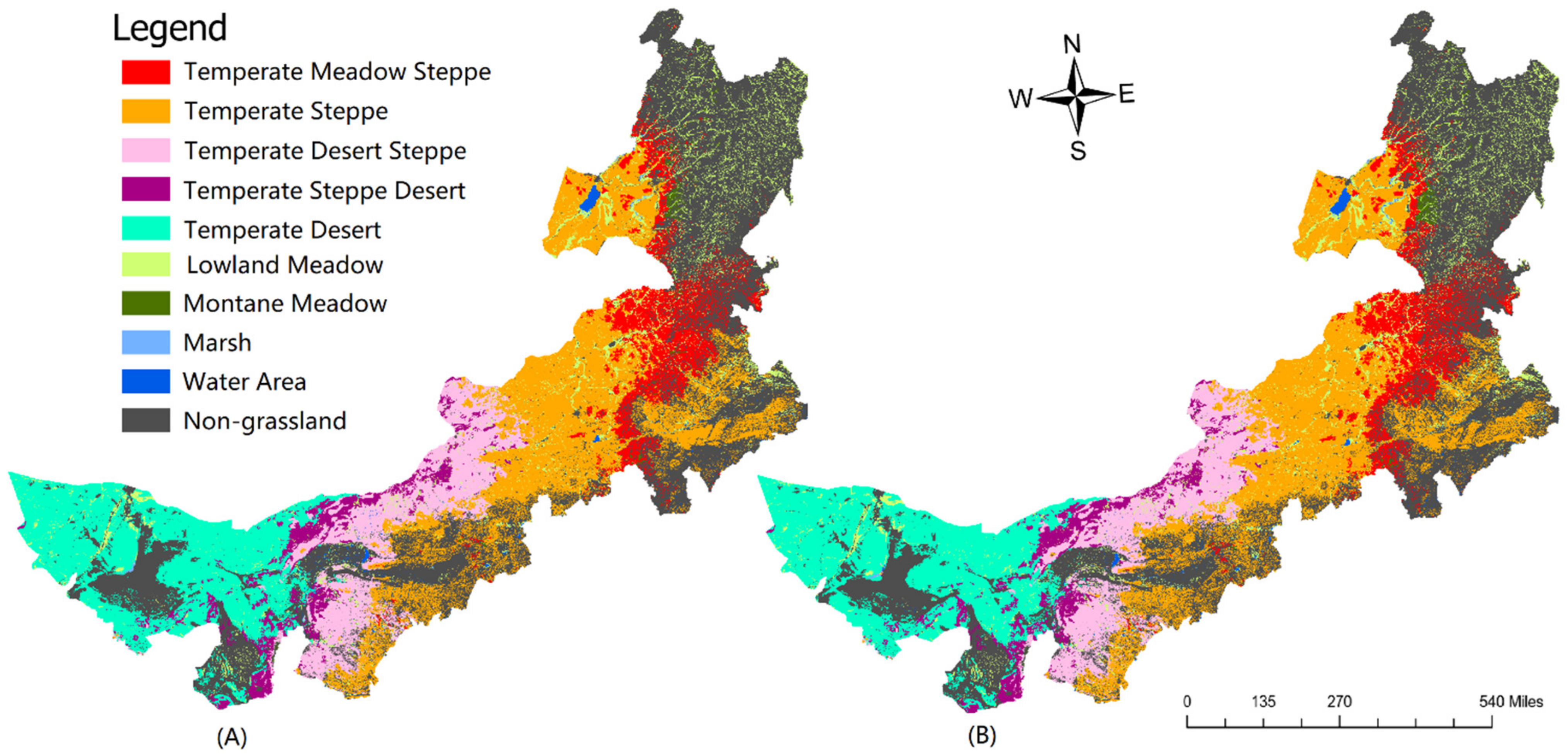
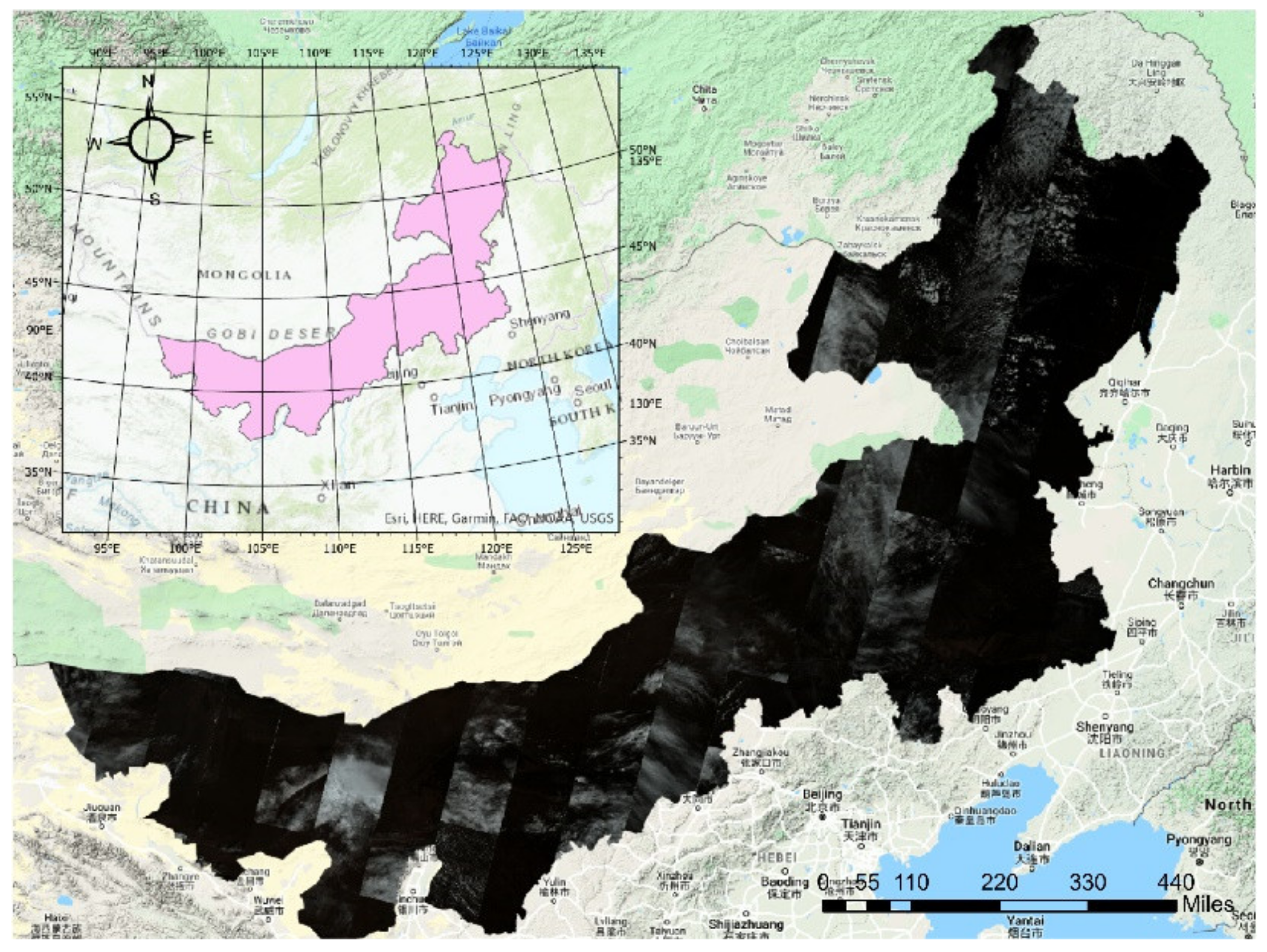
2.1. Study Area

The IMAR is located in northern China (Figure 1). It is the third largest province in China with 103 counties (or banners as named by the local Mongolian population). The overall area is about 1.18 million square kilometers extending from 37°24′ N to 53°23′ N and 97°12′ E to 126°04′ E. The shape of IMAR is long and narrow. The climate across the region is variable as the western part of IMAR is semi-arid, while the eastern and northern areas correspond to a semi-humid climate.

The major land cover in IMAR is grassland. The Hulunbeir Grassland, located in northern IMAR, is one of the largest natural grasslands in the world. In this study, we adopted the major vegetation types (10) identified in the 1:1,000,000 vegetation map of China as the LULC classes for our analyses (

Table 1. IMAR LULC classes including grassland subclasses.

Class ID	Classes	Subclass ID	Subclasses
1	Temperate meadow-steppe (TMS)	30011	Plain and hilly area of meadow steppe subclass
		30012	Mountain land of meadow steppe subclass
		30013	Sand land of meadow steppe subclass
2	Temperate steppe (TS)	30021	Plain and hilly area of steppe subclass
		30022	Mountain land of steppe subclass
		30023	Sand land of steppe subclass
3	Temperate desert-steppe (TDS)	30031	Plain and hilly area of desert-steppe subclass
		30032	Mountain land of desert-steppe subclass
		30033	Sand land of desert-steppe subclass
4	Temperate steppe-desert (TSD)	30070	Temperate Steppe-desert subclass
5	Temperate desert (TD)	30081	Gravel soil of desert subclass
		30082	Sand soil of desert subclass
		30083	Salt soil of desert subclass
6	Lowland meadow (LM)	30151	Lowland meadow subclass
		30152	Salinized lowland meadow subclass
		30154	Marshy lowland meadow subclass
7	Montane meadow (MM)	30161	Low-middle hills of mountains meadow subclass
		30162	Subalpine of mountains meadow subclass
8	Marsh (MA)	30180	Marsh
9	Water area (WA)	w	N/A
10	Non-grassland (NG)	f	Forest
		s	Sand
		r	Road
		1	Human land use and all others non-grassland

) [34].

In recent decades, researchers have studied IMAR with a focus on LULC classification [35], grassland degradation [36], ecosystem stability [37], long-term climate change trends [38], and net primary productivity [39]. In these studies, RS images from Landsat and MODIS were important data sources for both input and validation. However, the images were often affected by weather conditions and unable to generate products with acceptable quality owing to the high degree of gaps in the data. For example, the Landsat 8 OLI images in Figure 1 represent the best quality images available for August 2016. After running a cloud removal algorithm with band 9 of Landsat 8 as input, cirrus clouds are detected and removed. The data gaps are shown in Figure S1.

2.2. Data Availability

A high-accuracy LULC vector mapping dataset generated by visual interpretation assisted by sample plots was available for 2000, 2010, and 2016 for the IMAR region, and was used as a training and validation LULC dataset in this study [40]. An initial set of 26 land cover subclasses was reclassified into the ten land cover types introduced in Table 1. In addition, a 30 m spatial resolution DEM dataset was created using The Advanced Spaceborne Thermal Emission and Reflection Radiometer (ASTER) Global Digital Elevation Model (GDEM) program, and downloaded from the NASA Earthdata portal. Slope for this region was calculated by processing the DEM data. A roads and railways vector dataset was acquired from OpenStreetMap [41]. The distance from each cell to roads and railways was calculated as one of the suitability factors for LULC change. Meteorological data including annual precipitation and temperature were provided by the Chinese Meteorological Data Service Center [42] from 2000 to 2016. These data were interpolated and rasterized using AUSPLIN, a meteorological data processing framework with 981.757258 m as the cell size [43].

Population and livestock survey data from 2000 to 2016 were provided by the Department of Agriculture and Animal Husbandry, China. Population density and livestock density were calculated based on county vector data. County-based data on the eco-compensation policy that was in effect from 2010 to 2015 were also provided by the Department of Agriculture and Animal Husbandry, China.

3. Methodology

3.1. Workflow

In this study, we used historical LULC data from 2000 and 2010 as well as data from 2016 to train a Markov chain–CA model to fill gaps in the data record and simulate LULC data that were missing. Ecological, economic, demographic, and urban factors were integrated to facilitate sub-space analysis through computational data mining and localized model training to improve the accuracy of the simulation results. The workflow for the gap filling framework based on large-scale LULC involved seven major steps (Figure 2). The details of this workflow including each step are explained in the following sections.

3.2. LULC Data Preparation

The first step in the workflow was LULC classification, mapping, and auxiliary dataset preprocessing. For this research, the analysis of the entire IMAR region was considered as a large-scale study. For example, Landsat 8 OLI, a widely used, medium spatial resolution RS imagery dataset with a relatively short revisit period [44], was used to cover the entire IMAR. Approximately 190 scenes of images were needed for a complete coverage of IMAR. Three years of input data were used to test and validate our cloud-based Markov CA simulator. This data preparation involved processing approximately 600 scenes of Landsat 8 OLI images, including handling atmospheric correction, cloud removal, and mosaicking. The overall data input was over 1 TB, which precluded processing on a single workstation in a timely fashion [45]. In this study, therefore, exploiting a big data processing framework was a must.

Processing RS datasets and classifying them into LULC is an active area of study and many researchers have developed methods and frameworks to process large-scale RS images [46,47]. However, it is worth pointing out that all LULC classification and mapping tasks need to satisfy an accuracy assessment before being applied. The quality of input images, auxiliary data, and classification methods will all impact the final accuracy of LULC classification results. For this research, we directly applied already existing masked LULC maps from 2000, 2010, and 2016 as input for Markov chain training analysis and used the 2016 LULC data for validation. The highly accurate, already-classified LULC maps helped to better focus on the task of large-scale gap filling by using a cloud-based Markov CA. To derive measures of overall accuracy for the gap filling task, confusion matrices and Cohen’s Kappa statistics were calculated to determine the overall accuracy and consistency for this workflow.

3.3. Sub-Space Simulation by Adopting Data Mining Techniques

The second step of the workflow was to segment the large study area into relatively homogeneous sub-simulation-space (SSS) before models training, given that the environment, climate, and human activities varied across the study area. This process allowed the design of functions to be tailored to integrate both constraint and restraint factors for subregions with relatively similar impact factors, which can better calibrate and train the model for each region.

A county-based multivariate geographic k-medoids clustering analysis was performed [48]. LULC classes, DEM, slope, precipitation, and temperature were raster data. Population density and livestock density were county-based vector data. The majority value of the LULC was assigned to a county as the LULC type. For DEM, slope, precipitation, and temperature, the mean values were calculated for all cells in each county to generate the final values of these variables by counties. As population density and livestock density were county-based, no further preprocessing was needed. The multivariate clustering was implemented using ArcGIS Pro 2.5.0. To optimize the clustering strategies, different clusters were generated from 2 to 30 clusters. A Calinski–Harabasz pseudo F-statistic [49] was applied to rank the top three cluster candidates for further processing. This F-statistic generated a minimum spanning tree by calculating the within-group similarity and between-group differences. In other words, spatially contiguous areas were divided into clusters by maximizing the within-group similarities and between-group differences.

The third step was to select the best SSS segmentation strategy among multiple candidates generated from the previous step in the workflow. In this step, 10,000 random sample points across IMAR were generated. They were assigned values for each point based on LULC classes, DEM, slope, precipitation, temperature, population density, and livestock density. Then, 75% of sample points were randomly sampled as the training dataset, and the remaining 25% of sample points were used as the test dataset for discriminant analysis. In this study, a quadratic discriminant analysis (QDA) was applied to avoid the problem where the covariance matrix was not the same for all [50]. McLachlan also claimed that linear discriminant analysis (LDA) should be used cautiously because it is unlikely that homoscedasticity will hold exactly in real world modeling, even when the preliminary test does not reject the null hypothesis. After running the QDA, confusion matrices were generated and the overall accuracy was calculated. The overall accuracy for six clusters, seven clusters, and eight clusters was 92.37%, 89.52%, and 90.04%, respectively. Hence, the six-cluster strategy was selected to divide the IMAR into six sub simulation spaces (see Figure S2).

3.4. Implementing Cloud-Based Distributed Markov–CA Model

As the fourth and fifth steps in the workflow, a Markov model for each SSS was trained and a set of suitability grids were built using multi-criteria evaluation (MCE) that was applied to the LULC data. These two steps were integrated using Apache Spark, an open sourced framework that can support in-memory distributed large-scale data processing. Then, the CA model was run to add a spatial component. This involved applying a spatial neighborhood filter to assign weights to the suitability scores of each cell. The number of iterations was assigned at the initialization step. Once the CA processing started, it updated cells’ statuses with transition rules to decide the highest possible simulated transitions among each LULC class. This step was built using an iterative graph processing framework—Apache Giraph, which allows customized graph-based algorithms to be processed in the cloud environment. In the final (seventh) step, an accuracy assessment was run for the simulated results using the 2016 LULC data as validation. A detailed discussion for each step of this workflow is presented in the following sections.

3.4.1. Multi-Temporal Markov Processing for Filling Missing Data

Using Markov processing, the status of each cell at the same coordinates but from different input time steps was compared by overlaying two pairs of input LULC datasets: (1) 2000 LULC data to 2010 LULC data and (2) the gap-masked 2010 LULC data to the gap-masked 2016 LULC data. The gaps were the areas where there were missing data. The number of cells that convert from one LULC class to a different class over two temporal periods (2000–2010 and 2010–2016) was calculated. The transition probability matrix was generated using the following equations [19]:

$$P(X_{m+1}=j | X_m=i, X_{m-1}=i_{m-1}, \dots X_0=i_0)=P(X_{m+1}=j | X_m=i)$$

(1)

$$P_{ij}=P(X_{m+1}=j | X_m=i), m=0, 1, 2,\dots$$

(2)

where $X_m$ represents the random process; m = 0, 1, 2 represents the cell status at two different time steps; and $P_{ij}$ is the transition probability calculated using the following equation [17]:

$$P_{ij}=\frac{n_{ij}}{n_i}$$

(3)

where $n_{ij}$ represents the number of cells converted from class i to class j and $n_i$ represents the count of cells converted from class i to all other classes. Assuming there were n classes in this transition period, the values $p_{ij}$ in transition matrix were as follows:

$$0 \le p_{ij}<1 and {{\displaystyle \sum }}_1^n{p}_{ij}=1$$

(4)

where i and j are integers ranging from 1 to n. The cloud-based algorithm was implemented using Apache Spark on a cloud environment and using a MapReduce function. (Algorithm 1).

Algorithm 1 Distributed calculating probability matrix using Apache Spark

1: def Mapper (Key, Value)

2:     Foreach cell in LULC dataset:

3:     Emit (Cij, 1);

4:

5: def Reducer (Key, int[] Values)

6:     int SUM = 0;

7:     Foreach count in values:

8:       SUM += count;

9:     Emit (Cij, SUMij);

10:    Pij = SUMij/SUMTotal

11:    Emit (SUMij, Pij)

At the map stage, cells at the same coordinates from two different input LULC datasets were compared. C_ij represented the conversion from LULC class i to class j. Each pair was counted as 1. After this step, a list of all conversions was generated. At the reduce stage, all 1s from all computing nodes were summarized using C_ij as a key to calculate the SUM_ij, which represented the number of cells of each conversion pair. In other words, SUM_ij also represented the conversion area of each pair because the cell size was fixed. Then, the transition area matrix was generated and the transition probability matrix $P_{ij}$ was calculated using SUM_ij divided by SUM_Total, returning the total number of input LULC cells.

It should be pointed out that there were initially two multi-temporal transition probability matrices: the transition matrix from 2000 to 2010 and the transition matrix from 2010 to 2016. The latter was applied to calibrate the 2000–2010 transition matrix. Equal weights were empirically assigned. The rationale for an equal weight was that the 2000–2010 transition matrix represented the potential change over 10 years, while the 2010–2016 transition matrix showed changes over 6 years. The weights could be 10/16 and 6/16 from the time-series perspective. However, for the sake of filling the LULC gaps in 2016, the 2010–2016 transition matrix better represented the LULC change probabilities from 2010 to 2016. Through an iteration experiment, an equal weight for the two matrices generated the best matches with the validation results over the gap areas.

3.4.2. Localized Model Training to Fine-Tune Transition Rules

The cloud-based and distributed Markov–CA simulator can use localized ancillary data to train transition rules for calibrating the Markov–CA model over the SSS. One practical solution to optimize the simulated results was to apply suitability grid sets. Suitability grid sets contain the suitability values for each cell that may transition to a different LULC class. Suitability grid sets were calculated by the MCE method by assessing each involved constraint and restraint factor. The constraint suitability value was a Boolean type that contains values 0 and 1. Constraint suitability refers to the fact that a specific LULC class was not expected to change to another LULC class during the simulation. Those cells of unchangeable LULC regions were marked as 0 and the other locations in the study area were marked as 1, which represented the potential suitability for land cover change. For example, in IMAR, any type of grassland was highly unlikely to change into a water body over the course of a few decades. While over time, developed land use (i.e., human land use) in an area might see an expansion, but would be less likely to change back into a natural land cover. Hence, in this study, areas of water and human land use were considered as constraint factors.

The restraint suitability values were values in a normalized range calculated by the effect of each restraint factor, i.e., the potential suitability change level for a specific LULC class from unsuitable (small value) to highly suitable (large value). In this study, two constraints and nine restraint factors were involved, and the details for defining these factors are provided in

Table 2. Suitability factors.

Factors	Definition	Function Shape	Control Point (s)/SB
DEM	Elevation of whole IMAR (m)	MDJ	SSS 1	690, 1143
			SSS 2	387, 973
			SSS 3	1024, 1672
			SSS 4	1414, 1969
			SSS 5	1316, 1852
SLOPE	Slope calculated by DEM (degree)	MDJ	SSS 1	6.1, 20.5
			SSS 2	3.9, 17.3
			SSS 3	4.1, 14.9
			SSS 4	11.1, 27.7
			SSS 5	4.5, 15.8
DisRoad	Distance to roads	Linear	N/A
DisRail	Distance to railways	Linear	N/A
PPT	Yearly average precipitation (mm)	SS	SSS 1	389.35
			SSS 2	419.88
			SSS 3	276.29
			SSS 4	361.9
			SSS 5	152.4
TEMP	Yearly average temperature (centigrade)	SS	SSS 1	−1.58
			SSS 2	5.97
			SSS 3	3.28
			SSS 4	6.5
			SSS 5	8.38
POP	Population density per each county (people per km2)	MDJ	SSS 1	5.1, 37
			SSS 2	37.8, 338.1
			SSS 3	8.1, 194.5
			SSS 4	52.0, 379.4
			SSS 5	1.8, 57.5
LS	Livestock density per each county (livestock per km2)	MDJ	SSS 1	11.1, 74.9
			SSS 2	115.9, 474.6
			SSS 3	36.9, 240.6
			SSS 4	116.4, 521.2
			SSS 5	14.2, 138.9
CP	Compensation policy	Linear	0, 1, 2
WA	Water area	Boolean	N/A
LU	Human land use	Boolean	N/A

.

Restraint factors affected LULC change with specific functions and control points. For example, DisRoad and DisRail represented the distance to roads and railways. The closer roads and railways (i.e., short distances), the less chance there was that the original LULC classes would be converted into grassland classes. In this study, the effect of the distance to road and railways was defined as a linear function. Related to animal grazing practices in the study area, the compensation policy included three practices: normal grazing (not participated in), balanced grazing, and forbidden grazing. This was a county-based policy that allowed herdsman to receive compensation for balanced grazing or to halt grazing for specific time periods. Not all counties in IMAR participated in this program. In this study, a linear function was defined for this factor by considering that, with less grazing, there would be a higher chance that grasslands may recover from other types of LULC classes. Water areas (WAs) and human land use areas (LU) were two constraint factors that were not expected to change into grassland classes.

Different function shapes were also applied to optimize the suitability value calculations. In this study, four types of functions were applied in MCE: monotonically decreasing J-shaped function (MDJ), linear, symmetric sigmoidal (SS), and boolean. For example, in sub-simulation space (SSS) 1, a monotonically decreasing J-shaped function was used to calculate suitability values for the DEM layer. Control points defined the position and accurate shape of the function curve in the Cartesian coordinate system. Shape was used for cases such where, for example, the potential suitability of grassland was similar for areas with less than 690 m elevation. Suitability gradually decreased, however, as elevation increased from 690 m to 1143 m. Land was deemed unsuitable for grassland at elevations higher than 1143 m. Another example was a symmetric sigmoidal function that was used to calculate the values for the yearly average temperature layer. To simplify calculations, we set −1.58 °C as the uppermost value for average yearly temperature according to the average yearly temperature from 2010 to 2016, which represented that the grassland suitability value was highest at −1.58 °C, and gradually decreased with lower or higher temperatures. After processing all eleven suitability factors, a suitability grid set was generated with assigned weights for each suitability grid. In this study, we applied equal weights to all eleven factors to simplify the modeling and computing.

3.4.3. Fine-Tuned CA Simulation on the Cloud

In this study, the CA model was applied to undertake three tasks: (1) neighbourhood filtering that assigned different weights to target cells within the designated neighbourhood scheme; (2) computing a final transition value for each cell based on the transition probability matrix, transition area matrix, and suitability grid sets; and (3) defining iterations for time intervals within given time periods based on the input LULC datasets used in the simulation process.

However, to process a large-scale CA model (i.e., beyond the computational capacity of a single workstation) efficiently is a challenge. Some researchers have already explored this using big data computing frameworks and high-performance computing resources. For example, Radenski [51] tested such an algorithm on Amazon’s Elastic MR Cloud with a maximum 1.6 × 10⁸ cells in a 2D situation, where they employed 1 master node and 16 core nodes in this simulation. Marques and colleagues [52] developed a new computational framework based on MapReduce to implement a 1 trillion cell 2D CA simulation on the Microsoft Azure cloud platform. Those large CA approaches show the applicability of CA to big data/big model computing, but also leave room for other investigators to achieve improved solutions with simpler modeling, faster computing, and easier data access.

Our approach tackled this problem using a graph-based cellular automata implementation. We considered the graph as a highly suitable framework for big data/big model development as the CA model contained cells and their neighbors. Cells can be modeled by vertices, and neighbor relationships can be reflected in an edge pattern. By evaluating the state of vertices connected with a target vertex, users can easily set up the transition rules to update the state of the target vertex. More importantly, with graph-based CAs, we could make use of suitable and powerful large-scale graph processing infrastructure such as Apache Giraph in order to achieve massive cell volume and high performance with the CA simulation. Those infrastructures can be quickly deployed on cloud platforms such as Amazon Web Services (AWS) [53], Microsoft Azure [54], as well as Google’s Compute Engine [55]. All of them can offer potentially massive computing resources to support the research processing.

The algorithm to implement cloud-based CA that used Apache Giraph, a computational framework based on the bulk synchronous parallel (BSP) model, is illustrated in Algorithm 2.

Algorithm 2 Distributed processing CA model with Apache Giraph

1: class GiraphCA

2:      MaxSuperStep ← user defined value

3:      function compute (vertex, messages):

4:      if getSuperstep() == 0 then

5:        sendMessage to all neighbors, assign weight,

6:        compute (Eij = neighbor weight × suitability value)

7:        if getSuperstep() <= MaxSuperStep then

8:      Foreach cell in study area:

9:      While (true):

10:         if max(Eij) > area limit then

11:          max(Eij) = 0

12:         else

13:       convert i to j;

14:       break;

15:         end if

16:      else

17:       voteToHalt()

18:      end if

19:    end if

This framework contains many super steps (in terms of Apache Giraph) that are analogous to the timesteps in traditional CA terms. At each superstep, each computing unit is arranged into a certain number of vertices or edges that ensures parallel computing. Each computing unit communicates with others through message interaction. When the processing of this unit reaches a barrier, it stops until other cores complete their message interaction. After executing compute-functions in code for certain supersteps or certain halt conditions, users can save the output back to the distributed file system (DFS). The message-passing and barrier features are very useful in implementing CA approaches to support CA cell status changes based on neighbors and updates at each step. In this study, the neighborhoods of each target cell were calculated at superstep 0 by sending messages with designated edge patterns. Then, neighborhood weighted values were calculated and integrated with the results from MCE. Each cell’s overall evaluation value list in the study area (E_ij) was captured because each cell could possibly transition from one value/class to another. Once superstep 1 began, Giraph CA started to find the highest transition possibility for each cell by calculating the maximum value in the overall evaluation value list. At the same time, the value could not exceed the corresponding value in the area transition matrix to avoid over estimation. After all cell statuses were updated, the job was halted, and the results of simulated cell values for the study area were output.

3.5. Experiment Environment

The computational environment used in this research for the local cloud environment tests involved 1008 computing vcores and 5.12 Tb memory available. A 2 Pb HDFS was configured and the block size was 128 M as default (

Table 3. Computing environment.

Hardware				Software
Role	Count	CPU	RAM	Name	Version
Master Node	2	2× Intel Xeon E5-2680v4 2.4 GHz	256 G	Apache Spark	2.2.0
				Apache Giraph	1.2.0
Computing Node	18	2× Intel Xeon E5-2690v4 2.6 GHz	256 G	Centos	6.9
				Java Server VM	1.8.0_152 64Bit
Network	10 Gbps			Cloudera	5.12.0

).

The approach presented in this paper is based on YARN, which has been widely used in many current cloud environments [56].

4. Results

4.1. Simulation Results and Accuracy Assessment

For this analysis, masked LULC maps from 2000, 2010, and 2016 for IMAR were used as input training datasets to simulate and fill gaps in the 2016 dataset. With the computational capability of our cloud-based Markov–CA simulator, the entire IMAR was simulated with a single run. After completion, the simulated data for gaps were mosaiced with existing data on the 2016 LULC map to generate a final, estimated 2016 LULC map. Eleven impact factors from biophysical, ground features, and human-related factors were analyzed using MCE to build the suitability grids for the model. The transition rule matrix and its explanations are provided in Table S1.

The actual (observed) classified LULC result for 2016 and the simulated result for 2016 generated by the cloud-based Markov–CA were both mapped (Figure 3). We found the simulated results for the three major grassland types in IMAR meadow, steppe, and desert grassland were very close to their distribution in the actual LULC map. Especially, the TMS in the northeastern part of IMAR, and TDS and TD in the western part of IMAR showed high similarity based on visual assessment. The Greater Khingan forest, located in the northeast corner of IMAR, was classified into NG class in our study, and the simulated results were also visually close to the actual LULC case. Three water bodies, Hulun lake, Dalinur lake, and Ulansu Lake, were clearly represented. Major cities, major roads, and other types of human land use were also found to be similar based on visual inspection.

The overall accuracy assessment results were calculated using two commonly used accuracy assessment methods, a confusion matrix and Kappa statistic [57]. The accuracy assessment results for the model processed under four different scenarios were listed for comparison: (1) model processed using 2000 and 2010 data as input without using the SSS strategy (Table S2a); (2) model processed using 2000 and 2010 data as input using the SSS strategy (Table S2b); (3) model processed using 2000, 2010, and 2016 data as input without using the SSS strategy (Table S2c). In this case, a machine learning algorithm was adopted to correct the potential transitions in the transition matrix based on known transition trends from 2010 to 2016 using 2016 data; and (4) model processed using 2000, 2010, and 2016 data as input using the SSS strategy (Table S2d).

By calculating the confusion matrix and Kappa based on 20,000 sample points generated randomly across the gap areas in IMAR, the overall accuracy for Scenario 1 was found to be 81.23% and the Kappa statistic was 0.76. Next, the model was processed for Scenario 2, offering a 4% improvement in overall accuracy and 0.05 Kappa improvement. The model processed for Scenario 3 showed an additional 2.74% improvement in overall accuracy and 0.03 Kappa improvement compared with the model processed using 2 years of data and without using the SSS strategy. Finally, for Scenario 4, the overall accuracy improvement was 6.93% and the Kappa was improved by 0.09.

The simulated accuracy was also assessed for five sub-regions using a confusion matrix and Kappa statistic (Table S3). In those five sub-regions, the major grassland classes including TMS in sub-region 1, 3, and 4; TS in sub-region 1, 3, and 5; and TSD/TD in sub-region 3 and 5 were simulated with a high level of accuracy. Especially for TS in sub-region 1 and TDS in sub-region 3 and 5, the accuracy was over 99%. In sub-region 2, the accuracy of grassland was not as high (typically around 80%) as in other sub-regions owing to the rapid growth of cities and farmlands. The Kappa was 0.71 for sub-region 2 and 0.6 for sub-region 4, which were consistent across these regions.

The gaps filled by the Markov–CA simulator were mainly located in the eastern and northern parts of IMAR, owing to relatively high levels of moisture being present. To further assess the gap filling results, we analyzed three heavy cloud covered subareas (with over 85% gaps): the Hinggan League region in eastern IMAR, the Xilingol League region in the central part of the IMAR region, and the Bayan Nur region in the west. Each subarea covered approximately 100,000 square kilometers. Another reason for choosing these three areas was because three different grassland types were located in these areas: meadow grassland in the Hinggan League area, steppe grassland in the Xilingol League area, and desert grassland in the Bayan Nur area, providing a good basis for testing gap filling performance.

4.2. The Performance of Cloud-Based LULC Data Gap Filling Framework

As we discussed in previous sections, using cloud computing for LULC gap filling can significantly reduce the time costs for data acquisition, pre-processing, simulation, and results’ generation (

Table 4. Comparison of processing time between cloud-based LULC gap filling with traditional desktop based processing with commonly used software.

	Desktop (ArcGIS for Data Processing. IDRIS [58] for Markov-CA Simulation)	Cloud-Based Framework
Data acquisition	~600 Landsat 8 images covered the whole study area for three years. Assuming those images can be downloaded with 1 min each, it takes ~10 h in total	Can access directly from cloud storage such as S3. No time required
Data pre-processing	Assuming using ArcGIS to merge those images into three time periods and perform classification. The merge operation takes about 20 h with ~7 h each. The classification process is fully depended on the classifier. Using SVM as an example, it takes over 24 h for a single year image be processed	No need to merge data, can read data into memory from distributed file system directly include HDFS or S3. Can leverage cloud-based classification framework, which will take ~1 h.
Markov Chain	This is text-based processing. With Python script, it takes ~3 min. However, reading raster values takes extra time	Using Spark-based Markov chain, it takes ~20 s. No data reading time needed because it has been loaded into memory during data classification step.
Suitability analysis	Using IDRIS to process suitability maps, it takes over 24 h for the whole area	This process takes ~1.5 h to process with setup user-defined parameters into code.
CA process	Skip suitability process and apply CA process directly in IDRIS for performance test purpose only, it takes over 24 h for the whole area	This process takes ~2 h to finish gap filling and results filtering
Results’ visualization	Put text-based results into ArcGIS, it takes ~3 mins to show the results.	No time cost needed because results are designed as a PPM output, which is a text-based human readable figure.

).

Overall, we found that applying the cloud-based LULC data gap filling framework offered significant timesaving advantages especially for tasks involving a large study region. However, minor adjustments to parameters from the given study area are also required to perform the tailored simulation.

5. Discussion

Traditional gap-filling methods, including Markov chain CA models, are usually applied and processed on a single workstation with limited computational capacity and cannot support very large-area gap-filling tasks [10,11,12,13,14,15,32]. Our case study in IMAR intends to overcome this issue. We developed and implemented the distributed Markov chain CA model by exploiting cloud computing to address large area LULC gap filling in a reasonable time. Furthermore, our cloud-based LULC data gap filling framework is designed to fill missing data gaps over a vast study area, where the spatial disparity of LULC features is manifest. According to our experiments, the spatial disparity affected the final gap-filling results, and thus cannot be ignored. Hence, we proposed sub-simulation-space (SSS) strategies to address the influences of spatial disparity on missing data gap filling. As a result of this case study, we found that regional disparities must be carefully considered, especially for large-area Markov–CA simulations. The cloud-based Markov chain CA framework dramatically improved simulation accuracy by adopting localized ancillary data to divide the study area into sub simulation spaces (SSS) and enable localized model training for calibrating the model for each SSS. For example, the major LULC classes with improved accuracy were TMS, TS, TDS, and LM when sub-simulation-spaces (Scenario 2) were adopted. Apparently, the SSS strategy allowed tailored control processing on MCE. These results suggested that the accuracies of the simulated results with the sub-space analysis and the localized model training were higher and the results were more consistent [59]. Furthermore, TMS, TS, and TDS are major vegetation types in the entire IMAR and, subsequently, the data filling accuracies for these vegetation types were noticeable.

In addition, the classic Markov chain CA models use the past available data to train and obtain CA transition rules and apply these rules to simulate future states [17]. Usually, the simulated future states are not validated, thus these CA-based models belong to a type of metaphor model [19]. Our case study simultaneously advocated for spatial and temporal data mining to fine-tune CA transition rules. For the temporal data mining, we used the available data in 2016 to train transition rules to fill the missing data gaps in the same year, 2016. We trained and derived two transition matrices, 2000–2010 and 2010–2016. We then weighted the two transitions embedded in our distributed solution to significantly improve the accuracy of the results (Table S2d) compared with the traditional Markov chain CA model (Table S2a). From this point of view, our data filling algorithm is not simply simulating future states from past available data, but treating “the known future” as part of data mining. The known future here indicated the available information in the simulation year. Therefore, our new algorithm is genuinely filling the missing data gaps.

Using all the available data from 2000, 2010, and 2016, instead of only the first two years, to train the multi-temporal transition matrices improved the accuracy of gap filling. Using the entire IMAR as a study region, we were able to successfully test LULC gap filling strategies with the cloud-based Markov chain CA framework and successfully fill gaps in the 2016 LULC map, generating a complete LULC map for IMAR for 2016. Compared with the traditional Markov chain CA simulation, the multi-temporal Markov chain CA framework achieved a 6.93% improvement in overall accuracy (88.16%) and 0.09 Kappa improvement. Furthermore, TMS, TDS, and NG were the major LULC classes where the accuracy was improved owing to the fact that the available 2016 data mainly occurred in these regions. Therefore, the model was better trained using the transition trends from 2010 to 2016.

However, some issues were found with the simulated results. These issues occurred in the three areas with the most cloud coverage (and the most gaps to fill). The first simulated grassland subarea was in the Hinggan region (Figure 4A) and was compared to the actual LULC map of this area for 2016 (Figure 4B). In this area, TMS and TS were the two major grassland classes. The simulated results were similar to the actual surveyed grassland distribution in this area. However, the TS class was overrepresented to some extent, which may have resulted from the weight assignment and function control points setting for precipitation-related factors during the construction of the suitability grids. The spatial resolution for precipitation data (1 km) was lower than the spatial resolution of the LULC mapping (30 m). Hence, the control points for precipitation were generated by statistical methods, which might not have been able to represent the differences in precipitation in each part of this subarea. TS grassland might be sensitive to this environmental factor, and this may have resulted in the simulated TS grassland classes expanding faster than in reality.

It was also notable, in this area, that there was a lack of detailed simulation for the water body class. We found more WA class pixels existing (Figure 4A), but these pixels were changed into NG or other land cover types (Figure 4B). After checking the training data, the water body classes that were modeled in the simulated results existed in the 2010 LULC map. However, they were not classified as WA again in 2016 owing to dry up or a lack of water because they were small lakes or rivers that were vulnerable to an environmental change. The same issue occurred in the Bayan Nur region where the simulated result of Bayan Nur showed that the WA class was less-represented (Figure 4E) than it appeared in the actual LULC map of the same subarea (Figure 4F).

Human land use in IMAR was found to be under-simulated in the three subareas. Especially in the Xilingol League area, the simulated NG (non-grassland, i.e., human land use) (Figure 4C) was significantly less than the observed NG in this area (Figure 4D). For Xilingol, the major grassland classes were accurately simulated except for areas associated with human land use such as expanded cities and recently developed farmland. For example, the continuous NG area in the central part of Xilingo League was actually Xilinhot City. However, the simulated result for the area of Xilinhot City was smaller than the actual coverage. Moreover, some rectangular NG areas were also found in the southern part of this area, which were new farmlands developed in the past few years, but not successfully simulated in this study. This was mainly because of the fact that, although socio-economic impact factors such as population density, livestock density, and compensation policy data were integrated into the simulation process, further research on actual impact mechanisms and how those factors affect a population’s land use, as well as the best weight for each factor, is needed. For this reason, simulating human land use, especially farmland, was overall not as accurately simulated in the IMAR region as other land use types.

6. Conclusions

This paper presented a one-stop solution for LULC gap filling for a very large study region by integrating an Apache Spark-based in-memory distributed Markov chain and suitability processing algorithm, and a self-designed Giraph-based distributed cellular automata on the cloud. The advantages of this framework were as follows: (1) easy integration with existing cloud-based large-scale RS imagery processing tools, where the output can return a LULC dataset directly to a distributed file system on the cloud as input for the LULC gap filling task without additional data transfer; (2) improving traditional Markov–CA simulation performance by restructuring a CA-based on graph theory; (3) straightforward access to existing LULC and auxiliary data in a cloud data warehouse to construct CA simulation spaces and transition rule grids; (4) the capability to exploit large-scale cloud-based computing frameworks to accelerate processing speed; and (5) as with other cloud-based frameworks, this framework solution is able to gain unlimited computing resources (in theory) to support very large processing through commercial cloud computing platforms. In brief, the paper’s most innovative technological contribution is developing a data gap filling method for a big data set over a large area by integrating cloud and open-source computing techniques. Therefore, this data gap filling technique is suitable for global studies and applicable in many ecological, environmental, and geographical research fields that use remotely sensed data.

The paper also makes a novel methodological contribution to geoscience by enabling simultaneous spatial (sub-simulation spaces) and temporal data mining to fine-tune CA transition rules by incorporating rich socio-environmental ancillary information. Apparently, the accuracy of gap filling improves with the sub-simulation spaces strategy as well as with the temporal data mining strategy shifting from two years (2000, 2010) to three years (2000, 2010, and 2016). More importantly, the accuracy of gap filling improves more significantly when both spatial and temporal strategies are applied.

Further research is needed to design methods that continue to improve the accuracy and performance of this framework. For example, in IMAR, water bodies and human land use were not as accurately simulated as other LULC classes owing to a lack of supporting data and studies on the impact mechanisms for these classes. Moreover, weight assignments and function design require further study and need to be elaborated for each LULC class to help bring the final simulated results closer to the actual values. Analytic hierarchy process, a commonly used approach to assess the weight for each impact factor, will be integrated into this framework. The neighborhood scheme could also be adjusted and further tested. For example, different neighborhood sizes could also be applied along with an accompanying re-design of the computing partitioning of the Giraph-based CA to test the benefit on computing performance.

In addition, current temporal data mining approaches for fine-tuning CA transition rules are limited to three years (i.e., two simulation periods). Average weight is assigned to the two transition probability sets to compose the final transition probability set. This practice is ad hoc without a rigorous empirical validation or calibration procedure. The temporal data mining approach needs to extend to more simulation periods and integrate with a more scientifically sound approach to determine how each period transition probability will affect the composite temporal transition probability matrix.

References

1. Townshend, J.; Justice, C.; Li, W.; Gurney, C.; McManus, J. Global land cover classification by remote sensing: Present capabilities and future possibilities. Remote Sens. Environ. 1991, 35, 243–255. [Google Scholar] [CrossRef]
2. Dewan, A.M.; Yamaguchi, Y. Land use and land cover change in Greater Dhaka, Bangladesh: Using remote sensing to promote sustainable urbanization. Appl. Geogr. 2009, 29, 390–401. [Google Scholar] [CrossRef]
3. Liu, J.; Kuang, W.; Zhang, Z.; Xu, X.; Qin, Y.; Ning, J.; Zhou, W.; Zhang, S.; Li, R.; Yan, C. Spatiotemporal characteristics, patterns, and causes of land-use changes in China since the late 1980s. J. Geogr. Sci. 2014, 24, 195–210. [Google Scholar] [CrossRef]
4. Li, X.; Shen, H.; Li, H.; Zhang, L. Patch matching-based multitemporal group sparse representation for the missing information reconstruction of remote-sensing images. IEEE J. Sel. Top. Appl. Earth Obs. Remote Sens. 2016, 9, 3629–3641. [Google Scholar] [CrossRef]
5. Xing, J.; Sieber, R.; Caelli, T. A scale-invariant change detection method for land use/cover change research. ISPRS J. Photogramm. Remote Sens. 2018, 141, 252–264. [Google Scholar] [CrossRef]
6. Zeng, C.; Shen, H.; Zhang, L. Recovering missing pixels for Landsat ETM+ SLC-off imagery using multi-temporal regression analysis and a regularization method. Remote Sens. Environ. 2013, 131, 182–194. [Google Scholar] [CrossRef]
7. Gafurov, A.; Bárdossy, A. Cloud removal methodology from MODIS snow cover product. Hydrol. Earth Syst. Sci. 2009, 13, 1361–1373. [Google Scholar] [CrossRef] [Green Version]
8. Tseng, D.-C.; Tseng, H.-T.; Chien, C.-L. Automatic cloud removal from multi-temporal SPOT images. Appl. Math. Comput. 2008, 205, 584–600. [Google Scholar] [CrossRef]
9. Shen, H.; Li, X.; Cheng, Q.; Zeng, C.; Yang, G.; Li, H.; Zhang, L. Missing information reconstruction of remote sensing data: A technical review. IEEE Geosci. Remote Sens. Mag. 2015, 3, 61–85. [Google Scholar] [CrossRef]
10. Ballester, C.; Bertalmio, M.; Caselles, V.; Sapiro, G.; Verdera, J. Filling-in by joint interpolation of vector fields and gray levels. IEEE Trans. Image Process. 2000, 10, 1200–1211. [Google Scholar] [CrossRef] [Green Version]
11. Zhang, C.; Li, W.; Travis, D. Gaps-fill of SLC-off Landsat ETM+ satellite image using a geostatistical approach. Int. J. Remote Sens. 2007, 28, 5103–5122. [Google Scholar] [CrossRef]
12. Shen, H.; Zeng, C.; Zhang, L. Recovering reflectance of AQUA MODIS band 6 based on within-class local fitting. IEEE J. Sel. Top. Appl. Earth Obs. Remote Sens. 2011, 4, 185–192. [Google Scholar] [CrossRef]
13. Gladkova, I.; Grossberg, M.D.; Shahriar, F.; Bonev, G.; Romanov, P. Quantitative restoration for MODIS band 6 on Aqua. IEEE Trans. Geosci. Remote Sens. 2012, 50, 2409–2416. [Google Scholar] [CrossRef]
14. Melgani, F. Contextual reconstruction of cloud-contaminated multitemporal multispectral images. IEEE Trans. Geosci. Remote Sens. 2006, 44, 442–455. [Google Scholar] [CrossRef]
15. Zhang, J.; Clayton, M.K.; Townsend, P.A. Functional concurrent linear regression model for spatial images. J. Agric. Biol. Environ. Stat. 2011, 16, 105–130. [Google Scholar] [CrossRef]
16. Cheng, Q.; Shen, H.; Zhang, L.; Yuan, Q.; Zeng, C. Cloud removal for remotely sensed images by similar pixel replacement guided with a spatio-temporal MRF model. ISPRS J. Photogramm. Remote Sens. 2014, 92, 54–68. [Google Scholar] [CrossRef]
17. Halmy, M.W.A.; Gessler, P.E.; Hicke, J.A.; Salem, B.B. Land use/land cover change detection and prediction in the north-western coastal desert of Egypt using Markov-CA. Appl. Geogr. 2015, 63, 101–112. [Google Scholar] [CrossRef]
18. Baker, W.L. A review of models of landscape change. Landsc. Ecol. 1989, 2, 111–133. [Google Scholar] [CrossRef]
19. Fan, F.; Wang, Y.; Wang, Z. Temporal and spatial change detecting (1998–2003) and predicting of land use and land cover in Core corridor of Pearl River Delta (China) by using TM and ETM+ images. Environ. Monit. Assess. 2008, 137, 127. [Google Scholar] [CrossRef]
20. Weng, Q. Land use change analysis in the Zhujiang Delta of China using satellite remote sensing, GIS and stochastic modelling. J. Environ. Manag. 2002, 64, 273–284. [Google Scholar] [CrossRef] [Green Version]
21. Overmars, K.D.; de Koning, G.; Veldkamp, A. Spatial autocorrelation in multi-scale land use models. Ecol. Model. 2003, 164, 257–270. [Google Scholar] [CrossRef]
22. Pontius, R.G., Jr.; Chen, H. GEOMOD Modeling; Clark University: Worcester, MA, USA, 2006; Volume 44, pp. 1–45. [Google Scholar]
23. Ye, B.; Bai, Z. Simulating land use/cover changes of Nenjiang County based on CA-Markov model. In Proceedings of the International Conference on Computer and Computing Technologies in Agriculture, Wuyishan, China, 18–20 August 2007; pp. 321–329. [Google Scholar]
24. Mendes, R.L.; Santos, A.A.; Martins, M.; Vilela, M. Cluster size distribution of cell aggregates in culture. Phys. A Stat. Mech. Appl. 2001, 298, 471–487. [Google Scholar] [CrossRef]
25. Zhao, Y.; Billings, S.A.; Coca, D.; Ristic, R.; DeMatos, L. Identification of the transition rule in a modified cellular automata model: The case of dendritic NH4Br crystal growth. Int. J. Bifurc. Chaos 2009, 19, 2295–2305. [Google Scholar] [CrossRef] [Green Version]
26. Qiu, G.; Kandhai, D.; Sloot, P. Understanding the complex dynamics of stock markets through cellular automata. Phys. Rev. E 2007, 75, 046116. [Google Scholar] [CrossRef] [PubMed] [Green Version]
27. Xie, Y. A generalized model for cellular urban dynamics. Geogr. Anal. 1996, 28, 350–373. [Google Scholar] [CrossRef]
28. He, C.; Okada, N.; Zhang, Q.; Shi, P.; Li, J. Modelling dynamic urban expansion processes incorporating a potential model with cellular automata. Landsc. Urban Plan. 2008, 86, 79–91. [Google Scholar] [CrossRef]
29. Di Gregorio, S.; Kongo, R.; Siciliano, C.; Sorriso-Valvo, M.; Spataro, W. Mount Ontake landslide simulation by the cellular automata model SCIDDICA-3. Phys. Chem. Earth Part A Solid Earth Geod. 1999, 24, 131–137. [Google Scholar] [CrossRef]
30. Batty, M.; Xie, Y.; Sun, Z. Modeling urban dynamics through GIS-based cellular automata. Comput. Environ. Urban Syst. 1999, 23, 205–233. [Google Scholar] [CrossRef] [Green Version]
31. Fonstad, M.A. Cellular automata as analysis and synthesis engines at the geomorphology–Ecology interface. Geomorphology 2006, 77, 217–234. [Google Scholar] [CrossRef]
32. Guan, D.; Li, H.; Inohae, T.; Su, W.; Nagaie, T.; Hokao, K. Modeling urban land use change by the integration of cellular automaton and Markov model. Ecol. Model. 2011, 222, 3761–3772. [Google Scholar] [CrossRef]
33. Xie, Y.; Fan, S. Multi-city sustainable regional urban growth simulation—MSRUGS: A case study along the mid-section of Silk Road of China. Stoch. Environ. Res. Risk Assess. 2014, 28, 829–841. [Google Scholar] [CrossRef]
34. Hou, X. 1:1 Million Vegetation Map of China; National Tibetan Plateau Data Center: Beijing, China, 2019. [Google Scholar]
35. Lan, H.; Xie, Y. A semi-ellipsoid-model based fuzzy classifier to map grassland in Inner Mongolia, China. ISPRS J. Photogramm. Remote Sens. 2013, 85, 21–31. [Google Scholar] [CrossRef]
36. Tong, C.; Wu, J.; Yong, S.-p.; Yang, J.; Yong, W. A landscape-scale assessment of steppe degradation in the Xilin River Basin, Inner Mongolia, China. J. Arid Environ. 2004, 59, 133–149. [Google Scholar] [CrossRef]
37. Bai, Y.; Han, X.; Wu, J.; Chen, Z.; Li, L. Ecosystem stability and compensatory effects in the Inner Mongolia grassland. Nature 2004, 431, 181–184. [Google Scholar] [CrossRef]
38. Xie, Y.; Zhang, Y.; Lan, H.; Mao, L.; Zeng, S.; Chen, Y. Investigating long-term trends of climate change and their spatial variations caused by regional and local environments through data mining. J. Geogr. Sci. 2018, 28, 802–818. [Google Scholar] [CrossRef] [Green Version]
39. Wang, Z.; Zhong, J.; Lan, H.; Wang, Z.; Sha, Z. Association analysis between spatiotemporal variation of net primary productivity and its driving factors in inner Mongolia, China during 1994–2013. Ecol. Indic. 2019, 105, 355–364. [Google Scholar] [CrossRef]
40. IMIRSD. GIS Maps of Inner Mongolia Land Uses and Land Covers in 2000, 2010, and 2016; IMIRSD: Minnetonka, MN, USA, 2020. [Google Scholar]
41. OpenStreetMap. Available online: https://www.openstreetmap.org/ (accessed on 3 February 2020).
42. CMDC. Available online: http://data.cma.cn/data/ (accessed on 3 February 2020).
43. Hutchinson, M.F.; Xu, T. Anusplin Version 4.2 User Guide; Centre for Resource and Environmental Studies, The Australian National University: Canberra, Australia, 2004; Volume 54. [Google Scholar]
44. U.S. Department of the Interior. U.S. Geological Survey. Landsat 8. Available online: https://www.usgs.gov/landsat-missions/landsat-8 (accessed on 4 February 2020).
45. Lan, H.; Zheng, X.; Torrens, P.M. Spark Sensing: A Cloud Computing Framework to Unfold Processing Efficiencies for Large and Multiscale Remotely Sensed Data, with Examples on Landsat 8 and MODIS Data. J. Sens. 2018, 2018, 2075057. [Google Scholar] [CrossRef]
46. Teluguntla, P.; Thenkabail, P.S.; Oliphant, A.; Xiong, J.; Gumma, M.K.; Congalton, R.G.; Yadav, K.; Huete, A. A 30-m landsat-derived cropland extent product of Australia and China using random forest machine learning algorithm on Google Earth Engine cloud computing platform. ISPRS J. Photogramm. Remote Sens. 2018, 144, 325–340. [Google Scholar] [CrossRef]
47. Wang, N.; Chen, F.; Yu, B.; Qin, Y. Segmentation of large-scale remotely sensed images on a Spark platform: A strategy for handling massive image tiles with the MapReduce model. ISPRS J. Photogramm. Remote Sens. 2020, 162, 137–147. [Google Scholar] [CrossRef]
48. Ippoliti, C.; Candeloro, L.; Gilbert, M.; Goffredo, M.; Mancini, G.; Curci, G.; Falasca, S.; Tora, S.; di Lorenzo, A.; Quaglia, M. Defining ecological regions in Italy based on a multivariate clustering approach: A first step towards a targeted vector borne disease surveillance. PLoS ONE 2019, 14, e0219072. [Google Scholar] [CrossRef]
49. Caliński, T.; Harabasz, J. A dendrite method for cluster analysis. Commun. Stat.-Theory Methods 1974, 3, 1–27. [Google Scholar] [CrossRef]
50. McLachlan, G.J. Discriminant Analysis and Statistical Pattern Recognition; John Wiley & Sons: Hoboken, NJ, USA, 2004; Volume 544. [Google Scholar]
51. Radenski, A. Using MapReduce streaming for distributed life simulation on the cloud. In Proceedings of the Artificial Life Conference, Taormina, Italy, 2–6 September 2013; pp. 284–291. [Google Scholar]
52. Marques, R.; Feijo, B.; Breitman, K.; Gomes, T.; Ferracioli, L.; Lopes, H. A cloud computing based framework for general 2D and 3D cellular automata simulation. Adv. Eng. Softw. 2013, 65, 78–89. [Google Scholar] [CrossRef]
53. Amazon. Amazon Web Services. 2015. Available online: http://aws.amazon.com/es/ec2/ (accessed on 1 November 2020).
54. Wilder, B. Cloud Architecture Patterns: Using Microsoft Azure; O’Reilly Media, Inc.: Sebastopol, CA, USA, 2012. [Google Scholar]
55. Sanderson, D. Programming Google App Engine: Build and Run Scalable Web Apps on Google’s Infrastructure; O’Reilly Media, Inc.: Sebastopol, CA, USA, 2009. [Google Scholar]
56. Fan, X.; Lang, B.; Zhou, Y.; Zang, T. Adding network bandwidth resource management to Hadoop YARN. In Proceedings of the Seventh International Conference on Information Science and Technology (ICIST), Da Nang, Vietnam, 16–19 April 2017; pp. 444–449. [Google Scholar]
57. Congalton, R.G.; Green, K. Assessing the Accuracy of Remotely Sensed Data: Principles and Practices; CRC Press: Boca Raton, FL, USA, 2002. [Google Scholar]
58. Eastman, J.R. TerrSet Manual; Accessed in TerrSet Version; Clark Labs: Worcester, MA, USA, 2015; Volume 18, pp. 1–390. [Google Scholar]
59. Viera, A.J.; Garrett, J.M. Understanding interobserver agreement: The kappa statistic. Fam. Med. 2005, 37, 360–363. [Google Scholar] [PubMed]
Figure 1. Landsat 8 OLI images at IMAR from August 2016.
Remotesensing 14 00445 g001
Figure 2. Workflow for the cloud-based LULC gap filling process (Numbers 1, 2, 3, 4, 5, 6, and 7 correspond to the seven steps in the following text).
Remotesensing 14 00445 g002
Figure 3. Overall results. (A) Actual LULC mapping for 2016 and (B) LULC mapping with simulated gap filling for 2016.
Remotesensing 14 00445 g003
Figure 4. LULC maps of three grassland areas: (A) simulated Hinggan League area (meadow grassland), (B) real Hinggan League area, (C) simulated Xilingol League area (steppe grassland), (D) real Xilingol League area, (E) simulated Bayan Nur area (desert grassland), and (F) real Bayan Nur area.
Remotesensing 14 00445 g004