Article

Exploring the Intrinsic Probability Distribution for Hyperspectral Anomaly Detection

1
Department of Electrical Engineering, Zhejiang University, Hangzhou 310027, China
2
Department of Computer Science, Hangzhou Dianzi University, Hangzhou 310005, China
*
Author to whom correspondence should be addressed.
Remote Sens. 2022, 14(3), 441; https://doi.org/10.3390/rs14030441
Submission received: 30 November 2021 / Revised: 12 January 2022 / Accepted: 14 January 2022 / Published: 18 January 2022
(This article belongs to the Section Remote Sensing Image Processing)

Abstract

:
In recent years, neural network-based anomaly detection methods have attracted considerable attention in the hyperspectral remote sensing domain due to their powerful reconstruction ability compared with traditional methods. However, actual probability distribution statistics hidden in the latent space are not discovered by exploiting the reconstruction error because the probability distribution of anomalies is not explicitly modeled. To address the issue, we propose a novel probability distribution representation detector (PDRD) that explores the intrinsic distribution of both the background and the anomalies for hyperspectral anomaly detection in this paper. First, we represent the hyperspectral data with multivariate Gaussian distributions from a probabilistic perspective. Then, we combine the local statistics with the obtained distributions to leverage the spatial information. Finally, the difference between the test pixel and the average expectation of the pixels in the Chebyshev neighborhood is measured by computing the modified Wasserstein distance to acquire the detection map. We conduct the experiments on three real data sets to evaluate the performance of our proposed method. The experimental results demonstrate the accuracy and efficiency of our proposed method compared to the state-of-the-art detection methods.

1. Introduction

Due to the hundreds of continuous and narrow bands with a wide range of wavelengths, hyperspectral imagery (HSI) can provide much information about spectral signature [1]. The intensity of an object in HSI reflects the reflectance or radiance that mainly depends on the category of the object [2]. Therefore, it is possible to apply the unique spectral characteristic to distinguish different ground objects [3]. With the significant improvement of spectral resolution [4], HSI has been involved used in various domains such as aerial reconnaissance [5], military surveillance [6], and marine monitoring [7].
Hyperspectral anomaly detection is considered a particular case of target detection [8]. It requires no prior knowledge of background or specific objects compared to target detection tasks [9]. As a consequence, it owns a promising application prospect. The leading hyperspectral anomaly detection theory considers that the objects in HSI comprise the background component and the anomaly component [10]. Thus, it is rational to model hyperspectral anomaly detection as a binary classification problem. The anomalies we studied here are defined objects in small regions whose spectral signature significantly differs from the neighboring areas. Moreover, the processing strategies involved in this paper are based on the extraction of pixel-wise spectral representations using the variational autoencoder (VAE) [11]. Most of the objects in continuous areas belong to the background, while anomalies only occupy a small portion of the image [12]. Therefore, the distribution of anomalies is sparse [13].
Traditional hyperspectral anomaly detection methods pay much attention to the characteristic of background [14]. The landmark Reed-Xiaoli (RX) detector [15] assumes that the whole background obeys a multivariate Gaussian distribution. Based on the generalized likelihood ratio test, the Mahalanobis distance between the test pixel and the mean value of background distribution is calculated. When the distance is greater than a specific threshold, the hypothesis that the test pixel belongs to an anomaly can be verified. Two typical versions of RX, namely the global RX (GRX) detector and the local RX (LRX) detector, evaluate the background by global statistics and local statistics in HSI, respectively. However, it is difficult for all background objects to conform to a single normal distribution from a more general viewpoint. To overcome the limit, the work in [16] proposed the Kernel RX (KRX) algorithm that models the original data with a nonGaussian model in the high dimensional feature space. In addition, cluster and mixture model-based hyperspectral anomaly detection methods have been developed. A cluster-based anomaly detection (CBAD) algorithm assumes that the background pixel values within clusters can be modeled as Gaussian distributions, and anomalies have values that deviate significantly from the distribution of the cluster [17]. Reference [18] adopted a Gaussian mixture model (GMM) to describe the background statistics and incorporates a built-in mechanism for automatically evaluating the number of components. Besides that, a large variety of non-parametric methods have been proposed recently. The authors in [19] proposed a global anomaly detection algorithm based on the likelihood ratio test decision rule without any distributional assumption. Reference [20] presented a novel non-parametric high-dimension joint estimation algorithm for hyperspectral anomaly detection. The authors in [21] utilized the support vector data description (SVDD) strategy to implement fast anomaly detection. Furthermore, elliptically contoured distribution-based methods have been studied by researchers. The work in [22] presented an elliptically-contoured model for the distribution of background clutter. Reference [23] proposed a closed-form solution that optimizes the replacement target model when the background is a fat-tailed elliptically-contoured multivariate t-distribution.
Recently, with the development of compressed sensing technology in the signal processing domain, hyperspectral anomaly detection methods have been developed based on representation learning [24] and matrix decomposition theories [25]. Collaborative representation detector (CRD) [26] utilizes the conclusion that the background objects can be approximately represented by their local neighborhood, while the anomalies can not. Thus, the reconstruction error is leveraged to distinguish the anomalies from the background objects. Moreover, robust principal components analysis (RPCA) [27] method separates the original hyperspectral data into a background component and an anomaly component by implementing a simple matrix decomposition procedure [28], wherein the anomaly component is used for the following detection task. The method assumes that the background objects lie in a single subspace with no complicated implicit structure, whereas it is not realistic in most hyperspectral scenes. To surmount the constraint, Reference [29] proposed the low rank and sparse representation (LRASR) model by incorporating the low-rank representation (LRR) theory [30] into the sparse representation detector (SRD) [31]. LRASR employs the concept of background dictionary, which considers potential extensive categories of background objects. The nuclear norm constraint is added to the coefficients matrix of background to acquire the lowest rank representation of entire spectra jointly, and l 2 , 1 constraint is imposed on the anomaly part to make the distribution of anomalies sparse. However, the detection performance of the LRASR method mainly depends on the selection of the background dictionary. Furthermore, a low rank and sparse matrix decomposition (LSMAD) detector [32] inserts a noise term in the matrix decomposition procedure to alleviate the contamination simultaneously. A low-rank and sparse decomposition with mixture of Gaussian (LSDM-MoG) [33] exploits the variational Bayes technique to infer a posterior MoG model.
Apart from the methods above, novel detectors have been proposed based on neural networks in recent years. The convolutional neural network (CNN) based model [34] trains CNN by constructing the training sample pairs. Moreover, the autoencoder (AE) based frameworks have become prevalent due to their simplicity. Ref. [35] proposed a semi-supervised learning hyperspectral anomaly detection algorithm based on AE. The model trains the neural network with background samples according to the known ground truth. The anomaly pixels produce large reconstruction errors to separate them from the background objects. A robust graph AE (RGAE) [36] detector adds a l 2 , 1 norm to the reconstruction errors and embeds a graph regularization term. However, regardless of AE-based or CNN-based models, no consideration is attached to local spatial information that makes a big difference in hyperspectral anomaly detection. To address this issue, Ref. [37] incorporate the embedding manifold constraint into AE to sufficiently utilize the local structural information. Besides, the literature [38] is the first method to apply VAE to anomaly detection tasks. Despite the high reconstruction ability of VAE [39], the intrinsic probability distribution cannot be thoroughly explored. Table 1 summarizes the category and characteristics of hyperspectral anomaly methods.
Recently, most neural network-based anomaly detection methods have paid considerable attention to the reconstruction error. However, they neglect the useful low-dimensional information in the feature space. Ordinary AE and VAE based methods exploit the reconstruction error to distinguish the anomalies from the background. Therefore, intrinsic structural information about the joint distribution of anomalies and background cannot be leveraged. The motivation of this paper is to discover the probabilistic properties of hyperspectral data from a probabilistic perspective and explore a valid representation for both anomalies and background.
In this paper, we propose a novel probability distribution representation detector (PDRD) based on VAE structure for hyperspectral anomaly detection, which explicitly represents the HSI with multivariate Gaussian distributions and detects the anomalies by employing the modified Wasserstein distance. The VAE structure is adopted to acquire the representation of training samples. The outputs of the encoder, including the mean value vector and the standard deviation vector, jointly constitute a multivariate Gaussian distribution in the latent feature space. Then, we integrate the spatial information with the obtained distribution for each pixel by introducing the concept of Chebyshev neighborhood. For each pixel in the spatial space with its corresponding probability distribution, we define its Chebyshev neighborhood and compute the average expectation distribution of the pixels in the neighborhood to estimate the local statistics. Finally, we employ the modified Wasserstein distance to evaluate the difference between the test pixel and the average expectation distribution of the pixels within the neighborhood. In this way, we combine both spectral and spatial information to obtain the final detection results.
The main contributions of the paper can be concluded as follows.
(1)
We propose a framework to represent both the background and the anomalies in HSI by multivariate Gaussian distributions. The probabilistic characteristics of all objects can be discovered in the latent space.
(2)
Instead of exploiting reconstruction error, we integrate local statistics with probabilistic structural information by constructing the Chebyshev neighborhood for each pixel.
(3)
We build a valid criterion according to the actual property of HSI to evaluate the difference between two probability distributions, which highlights the anomalies and suppresses the background pixels.
The remainder of this paper is organized as follows. Section 2 briefly introduces the related work. In Section 3, we elaborate on our proposed method. Experimental results on three data sets are presented in Section 4. Finally, Section 5 draws the conclusion.

2. Related Works

The VAE model is a typical generative neural network that has been broadly applied in computer vision tasks. It estimates the probability distribution of the training data and then samples examples from the learned probability distribution, aiming to generate new images that look similar to the original data. Unlike the original AE framework, VAE views the reconstruction problem from a probabilistic perspective.
For each sample x , the goal of VAE is to maximize the likelihood function P ( x ) . According to the law of total probability, P ( x ) is represented as:
P ( x ) = z P ( x | z ) P ( z ) d z
where z indicates the latent variable to describe the implicit probability distribution. P ( x | z ) is intractable in the actual calculation procedure, thus variational inference is imposed to solve the dilemma. The loss function of VAE is then modeled by:
L = 1 N i = 1 N ( E q ϕ ( z | x i ) log p θ ( x i | z ) KL ( q ϕ ( z | x i ) p θ ( z ) ) )
where ϕ and θ denote the parameters of the encoder and decoder, respectively. N indicates the total number of training samples. The first term is called reconstruction likelihood, which measures the log-likelihood log p θ ( x i | z ) of sampling from q ϕ ( z | x i ) . The second KL-divergence term is usually called complexity constraint. It avoids the estimated posterior q ϕ ( z | x i ) deviating from the prior p θ ( z ) too much. The objective function of VAE ensures reconstruction accuracy, along with the generative ability of the model.
The main difference between the AE and the VAE is that the coding of AE is specific, whereas the coding of VAE is probabilistic. Therefore, the advantage of VAE is that it can extract the probability representation of each sample. For a given sample x , the probabilistic encoder generates the mean value vector and standard deviation vector in the latent feature space. To reconstruct x from the latent space, we combine these two vectors with a random term and feed them into the decoder network. For traditional images, VAE has achieved a satisfactory effect on anomaly detection problems [40].
Ordinary neural network-based methods regard the reconstruction error as an essential term in anomaly detection tasks. The detection process is achieved based on the reconstruction error. Due to the sparse characteristic of anomalies, the background pixels make a more significant difference during the training. Therefore, the background pixels yield low reconstruction error, whereas the anomalies yield high reconstruction error. However, the latent information in the feature space of the samples is ignored, which heavily limits the practical application. In our proposed method, we regard the VAE architecture as a feature extractor. As the network cannot well recover the anomalies, the latent features (including mean value and standard deviation) of anomalies behave differently from that of the background pixels. Therefore, the latent data can enhance the discrimination between the anomalies and the background pixels.

3. Methodology

In this section, we elaborate on our proposed method based on the VAE architecture. As illustrated in Figure 1, the proposed PDRD comprises three steps: (1) represent each pixel by a multivariate Gaussian distribution in the latent space; (2) select local Chebyshev neighborhood for each pixel to leverage the spatial information; (3) obtain the detection map by computing the modified Wasserstein distance between the corresponding distribution of the test pixel and the average expectation of its Chebyshev neighborhood.

3.1. Probability Distribution Representation

3.1.1. The Framework

Figure 1 illustrates the whole framework of our proposed method. First, the training sample x i R B is fed into the encoder module Enco. The training samples includes all pixels of the images. Next, the output of Enco is fed into the probability representation part PR to generate the mean value vector and standard deviation vector. Then, we combine these two vectors with the sampling module Samp to produce a specific sample. Finally, the decoder module Deco reconstructs the original data from the computed sample. The last epoch model is applied for the following feature extraction. Specifically, the proposed network mainly comprises the four modules that take on unique responsibilities. Enco denotes the encoder module that comprises three fully connected layers with 400 nodes. PR is the probability representation part, which consists of the mean value module and the standard deviation module of the training sample. Both of the modules comprise a single layer with 20 nodes. These two outputs constitute the Gaussian distribution of the data in the latent feature space. Samp represents the sampling module, which converts the probability distribution ( μ i and σ i ) to a specific sample by imposing a random term ϵ i . Deco comprises six fully connected layers with 20 nodes. The optimizer we use for the experiments is Adam, and the number of training epoch is 5.
Figure 2 shows the VAE network to characterize each sample with a Gaussian distribution. The VAE structure seeks to construct a latent variable that reflects the features of the image in some aspects when exploring the latent representation in the probabilistic space. Therefore, we regard the latent distribution as the probabilistic representation of the original data. Then, the reconstructed image is generated by sampling from the latent distribution. In this paper, we creatively exploit the Gaussian distribution in the latent space to explicitly express the whole image, which significantly promotes the convenience of exploring the latent characteristics.

3.1.2. Implementation of Dimensional Independence

Different dimensions in the feature space signify different latent attributes of the original image. However, there is no explicit meaning such as size, width, or angle for each dimension corresponding to the HSI. Instead, each pixel acts as a training sample fed to the neural network, which substantially differs from the ordinary optical image. Thus, the latent dimensions denote more intrinsic structural meanings at a deeper level. Theoretically, when the number of latent dimensions is fixed, independent dimensions can convey more information about the original data than dependent dimensions. Therefore, it is possible to enhance the discrimination between the anomalies and the background pixels. Furthermore, the disentangled latent representations can simplify the computation of Wasserstein distance, and it will be introduced in the following subsection.
For a pixel x i in HSI X = x i i = 1 N R B × N , the encoder extracts the approximate posterior distribution q ( z | x ) from PR , which consists of the mean vector μ and standard deviation vector Σ of the multivariate Gaussian distribution in the latent space. However, each dimension of the distribution is not strictly independent of each other, causing a high computational cost of calculating the Wasserstein distance. For example, for the distribution q ( z | x ) R k , it is equal to j = 1 k q ( z j | x ) when the whole dimensions of z are mutually independent. Thus, the difference between q ( z | x ) and j = 1 k q ( z j | x ) can evaluate the correlation between different dimensions. Hence, we strive to achieve dimensional independence for the simplicity of the following detection process.
The loss function acts as the optimization goal of the entire network. In other words, we can reshape our loss function to optimize the framework towards the desired orientation. By adding a weight coefficient [41], the expression of the loss function in (2) changes to:
L = 1 N i = 1 N ( E q ϕ ( z | x ) log p θ ( x i | z ) β · KL ( q ϕ ( z | x i ) p θ ( z ) ) )
Moreover, the KL divergence term in Equation (3) can be written in the form of expectation by [42]:
E p ( n ) [ KL ( q ( z | n ) | | p ( z ) ) ] = KL ( q ( z , n ) | | q ( z ) p ( n ) ) ( i ) Index-code MI + KL q ( z ) j q z j ( ii ) Total Correlation + j KL q z j | | p z j ( iii ) Dimension-wise KL
where random variable n indicates the index of selected training pixel, and it obeys a uniform distribution p ( n ) . We can see from Equation (4) that the newly constructed loss function contains the term (ii) called total correlation, and the expression owns the ability to evaluate the dimensional correlation. Therefore, to reduce the total correlation term to the greatest extent, the optimization emphasis should focus on the KL divergence term rather than the expectation term in Equation (3) from a global viewpoint. The optimization balance is broken up while enhancing the value of β , and the KL divergence term receives more attention in the optimization process. Dimensional correlation declines gradually as the weight parameter β increases, and it finally falls to a low level where it can be considered negligible. Therefore, the existence of β makes the relations of different dimensions disentangled, and the dimensional independence can be satisfied. Consequently, the discrimination between the anomalies and background pixels is enhanced, and the computation of Wasserstein distance can be simplified.

3.1.3. Selection of Chebyshev Neighborhood

After the probability representation step for each pixel, we acquire the independent multivariate Gaussian distribution in the latent space. In this way, the spectral information is fully exploited. Due to the robust local applicability of probability distribution, we seek to combine the spatial information with the obtained distributions.
Given a test pixel t with the two-dimensional (2D) spatial coordinate ( x , y ) , we define the point set V with ϵ Chebyshev neighborhood by:
V t l = { ( i , j ) | max ( | x i | , | y j | ) ϵ }
where l represents the index of points to be selected, and it ranges from 1 to the size of the neighborhood. ( i , j ) denotes the coordinate of the point that satisfies Equation (5). Figure 3 shows a simple example when ϵ equals 1.
As mentioned before, each pixel corresponds to a definite multivariate Gaussian distribution in the latent feature space. To approximate the local statistics of the test pixel, we introduce a random variable X ¯ t N μ , Σ that reflects the average expectation of ϵ Chebyshev neighborhood for the test pixel, and it can be characterized by:
μ ¯ t = 1 N i V t μ i
Σ ¯ t = 1 N d i a g i V t σ 1 i 2 , i V t σ 2 i 2 , , i V t σ k i 2
where μ i indicates the mean value vector of the distributions of the i-th pixel in V t , σ k i denotes the standard deviation of the k-th dimension of i-th pixel in V t .

3.2. Anomaly Detection with Modified Wasserstein Distance

3.2.1. Measurement of Different Distributions

In this step, we measure the dissimilarity of corresponding distributions between the test pixel and the average expectation of its Chebyshev neighborhood. In this paper, the concept of Wasserstein distance is adopted to measure the distinction between two distributions, which is also employed in generative adversarial networks (GAN) to alleviate the vanishing gradient [43].
For two acquired Gaussian distributions p = N 1 μ 1 , Σ 1 and q = N 2 μ 2 , Σ 2 on R k , with respective mean value vectors μ 1 and μ 2 R k , and symmetric positive semi-definite covariance matrices Σ 1 and Σ 2 R k × k , the Wasserstein distance between p and q is given by [44]:
W p , q 2 = μ 1 μ 2 2 2 + TR Σ 1 + Σ 2 2 Σ 1 Σ 2 1 2
where TR · denotes the trace of a matrix. The computation of Equation (8) is troublesome due to the complicated expression of the covariance matrix with high dimensionality. Figure 4 depicts the principles of coordinate-wise distance and Wasserstein distance. Unlike coordinate-wise distances, Wasserstein distance focuses on the optimal transport way between two distributions, and it is exploited to describe the structural differences.
By observing the expression of Equation (8), we know that the relationship among different dimensions of z makes a considerable difference. As the above analysis demonstrates, all dimensions of z are mutually independent, then Σ degenerates into a diagonal matrix denoted by:
Σ 1 = d i a g σ 1 2 , σ 2 2 , , σ k 2 Σ 2 = d i a g ϕ 1 2 , ϕ 2 2 , , ϕ k 2
where σ i and ϕ i , ( i 1 , 2 , k ) represent the standard deviation of each dimension for Σ 1 and Σ 2 , respectively. When the dimensional independence is satisfied, Equation (8) can be simplified to following equation:
W p , q 2 = μ 1 μ 2 2 2 + σ ϕ 2 2
where σ = σ 1 , σ 2 , , σ k T and ϕ = ϕ 1 , ϕ 2 , , ϕ k T . Therefore, the disentangled latent representations simplify the mathematical derivations and expressions, and it is tractable to evaluate the difference between the probability distributions p and q.

3.2.2. Modified Wasserstein Distance

As Equation (10) suggests, the standard deviation shares equal significance with the mean value. However, in real hyperspectral scenes, pixel intensity fluctuations of different categories are much greater than that of the same category. Therefore, the background pixels and anomalies mainly behave differently in their mean value. To reshape the mutual relationship of the two terms and better capture the distinctions, we attach a weight parameter γ to the standard deviation term as follows:
W p , q 2 = μ 1 μ 2 2 2 + γ · σ ϕ 2 2
Thus, it is tractable to measure the anomalous degree of the test pixel by computing the modified Wasserstein distance between the distribution of the test pixel and the average expectation distribution of the pixels in the ϵ Chebyshev neighborhood. The larger value of the computed Wasserstein distance indicates the higher degree of deviation from the average expectation for the test pixel. Accordingly, the pixel is more likely to be an anomaly. By reshaping the computed distance vector, we obtain the final detection map. The overall description of the PDRD algorithm is given as Algorithm 1.
Algorithm 1 Anomaly detection for HSI based on PDRD
Input: Training samples X R B × N and parameters: (1) trade-off parameter β and weight parameter γ ; (2) Chebyshev neighborhood ϵ ; (3) dimensionality k of latent distribution.
Output: Anomaly detection map.
  1:
Train a VAE neural network with modified loss function;
  2:
Extract the probability distribution for each training sample in the latent space;
  3:
Calculate the average expectation for each pixel according to its corresponding Chebyshev neighborhood;
  4:
Compute the modified Wasserstein distance between the corresponding distributions of the test pixel and the average expectation of the pixels in the ϵ Chebyshev neighborhood via Equation (11);
  5:
Reshape the computed distance vector to obtain the final detection map.

4. Experimental Results

4.1. Hyperspectral Data Sets

In order to evaluate the superiority of the proposed method, we conducted experiments on three different hyperspectral images. These three data sets are commonly used in hyperspectral anomaly detection, as the anomalies are representative and the number of background components is appropriate. Therefore, it is tractable to discriminate the performance among different detectors.

4.1.1. Pavia City Data Set

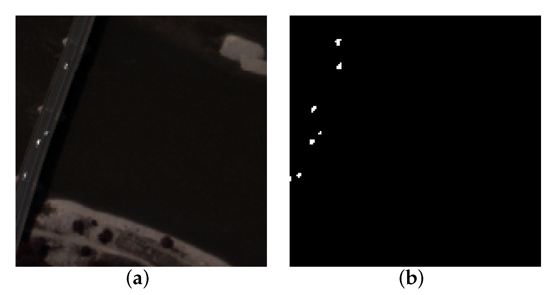
The hyperspectral data set was collected by the reflective optics system imaging spectrometer (ROSIS) sensor, which covered the city center of Pavia in northern Italy. It has 205 spectral channels, covering the wavelength ranging from 430 to 860 nm, along with a spatial resolution of 1.3 m. The image has a geometric size of 150 × 150 pixels. The 2D visualization of the Pavia City data set and the corresponding ground truth are shown in Figure 5a,b.

4.1.2. Gulfport Data Set

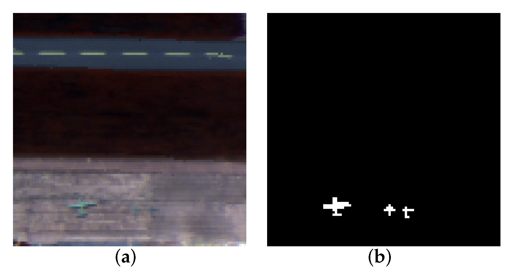
The data set was captured by the AVIRIS sensor over the airport area of Gulfport, MS, USA. The spatial resolution is 3.4 m, and the spatial size is 100 × 100 pixels. It contains 191 spectral channels spanning the wavelength of 550 to 1850 nm. In the scene, three planes of different sizes are regarded as anomalies. The main background of the image includes roads, vegetation, and runways. The 2D visualization of the Gulfport data set and its corresponding ground truth are depicted in Figure 6a,b.

4.1.3. Jasper Ridge Data Set

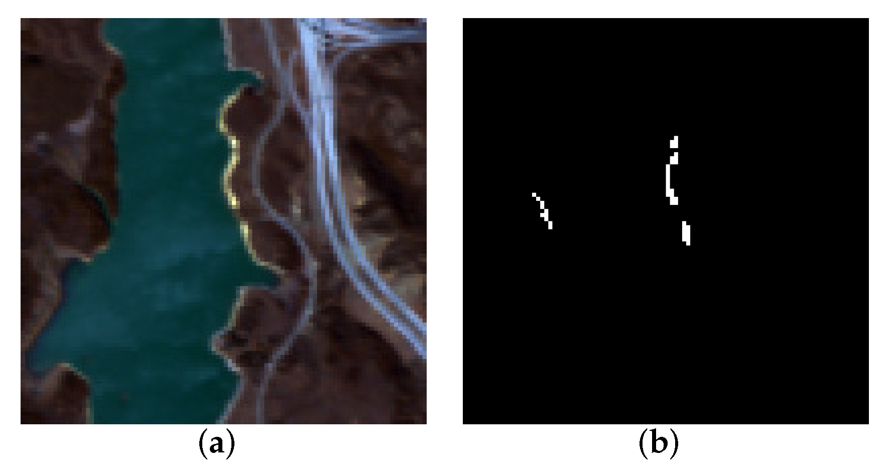
It is a popular hyperspectral data set acquired by the AVIRIS sensor over Jasper Ridge in central California. The spectral resolution is up to 9.46 nm. The image records 224 channels ranging from 380 to 2500 nm. After eliminating the bands 1–3, 108–112, 154–166, and 220–224 (due to dense water vapor and atmospheric effects), the remaining 198 channels are exploited for our experiment. The original image has a spatial size of 512 × 614 pixels, and a sub-image of 100 × 100 is used for the experiment. Since the original ground truth holds the modality of probability, several contaminated objects that possess an ambiguous category are chosen as anomalies. The main background components are water, roads, dirt, and trees. The pseudocolor image of Jasper Ridge data and its corresponding ground truth are shown in Figure 7a,b.

4.2. Competitors

The following state-of-the-art methods are compared with our proposed method.
(1)
GRX [15] is a benchmark hyperspectral anomaly detector. It assumes that the background satisfies a multivariate Gaussian distribution. The background is estimated using the entire image.
(2)
CBAD [17] partitions the image into several clusters and compute the distance between each pixel and the centroid of the pixel belongs to.
(3)
LRASR [29] adopts a background dictionary that can fully discover the implicit background structure in the latent subspace by low rank and sparse representation. The separated anomaly part is exploited to detect anomalies.
(4)
LSMAD [32] decomposes the original data into a background part, an anomaly part, and a noise part. The Mahalanobis distance that reflected background signature is computed for the following detection process.
(5)
LSDM-MoG [33] models the noise component with a mixture of Gaussian distributions. The anomalies are separated from the noise components by variational Bayes.
(6)
AE [35] attempts to recover the background pixels by the structure of neural network. The anomalies hold larger reconstruction errors than the background pixels, which is the principle to distinguish the anomalies from the background.
(7)
RGAE [36] imposes the l 2 , 1 norm to the reconstruction error and embeds a superpixel segmentatio-based graph regularization term into AE.

4.3. Detection Performance

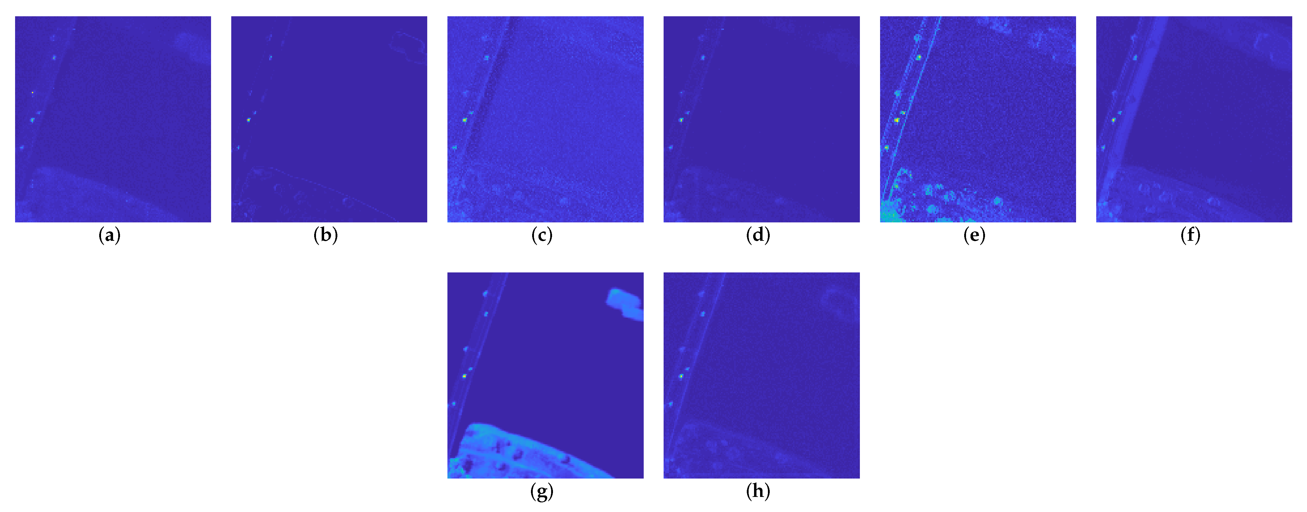
Receiver operating characteristic (ROC) curve serves as a valid criterion in hyperspectral anomaly detection tasks. The superiority and effectiveness of our proposed method are illustrated by comparing the ROC curves. In addition, the area under ROC curve (AUC) is used to evaluate the detection performance quantitatively. Furthermore, the visualization detection results are displayed to directly evaluate the performance, as Figure 8, Figure 9 and Figure 10 show.

4.3.1. Results of Paiva City Data Set

The visualization of detection results for Pavia City is shown in Figure 8. LSDM-MoG highlights both the background and the anomalies, leading to a high false alarm rate. As for RGAE, the detected anomalies contain many background pixels due to their large detection values. Several anomalies of GRX, LRASR, and LSMAD yield tiny values, causing a low detection rate. Although the background suppression is effective for CBAD, the anomalies are also evidently suppressed. Furthermore, the detection performance of AE is unsatisfactory because several bridge objects are detected as anomalies. Our proposed method fully utilizes global information of the data and incorporates the strength of local characteristics into the detection process to enhance the saliency of anomalies. In the detection map of the proposed method, we can see that the anomalies are well detected, and the false alarm rate is very low, which suggests the proposed method is superior to other methods.
As Figure 11a shows, ROC curves are plotted for Pavia City to compare the detection performance qualitatively. Notably, our proposed method always lies in the upper-left corner of the figure, indicating the powerful detection ability. Moreover, PDRD is the fastest to reach the position where the probability of detection equals 1. In the preliminary stage, the proposed PDRD dominates the detection probability with a value larger than 0.5. When the probability of detection approaches 1, the false alarm rate is less than 1 0 2 , which precedes other methods by a large margin. Moreover, as Table 2 displays, the AUC score of our proposed method is 0.9993, which is very near to 1. The value is convincing because it is consistent with the analysis of detection results and ROC curves.

4.3.2. Results for Gulfport Data Set

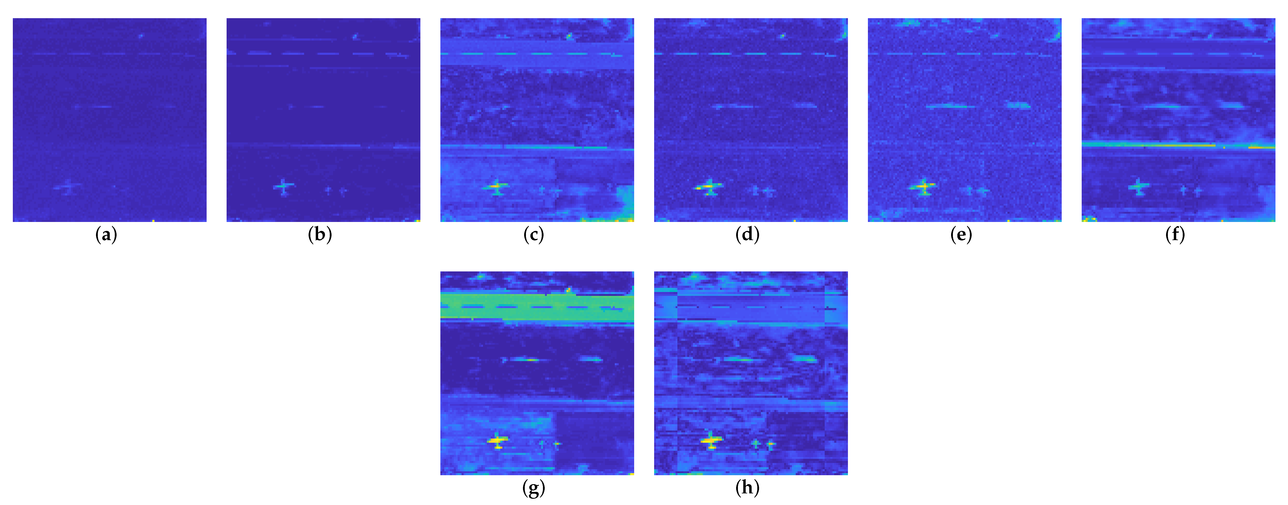
Figure 9 shows the visualization of detection maps for the Gulfport data set. In total, RGAE yields the worst detection performance among these detectors due to the evident stripes at the top of the image. LRASR wrongly detects a few background pixels as anomalies in the bottom-right corner of the image. AE incorporates a number of the runway objects into anomalies, and several horizontal stripes are significant. GRX and CBAD fail to detect a few anomalies, causing bad detection performance. Besides, some background pixels of LSMAD and LSDM-MoG are salient than anomalies, which largely influence the detection rate. The proposed method can detect all anomalies with significant intensity, indicating the most powerful detection ability among these methods.
ROC curves are plotted as shown in Figure 11b for the Gulfport data set to confirm the detection performance qualitatively. At the beginning, the detection rate of PDRD is over 0.4, which is the largest among these detectors. The ROC curve of our proposed method keeps at a high level since the false alarm rate is over 1 0 3 , and the speed of growth holds quite considerable.
For the Gulfport data set, our method achieves the best AUC score, which can be owed to integrating local information into global information of the data. The results are consistent with the evaluation of both ROC curves and the visualization of detection maps.

4.3.3. Results for Jasper Ridge Data Set

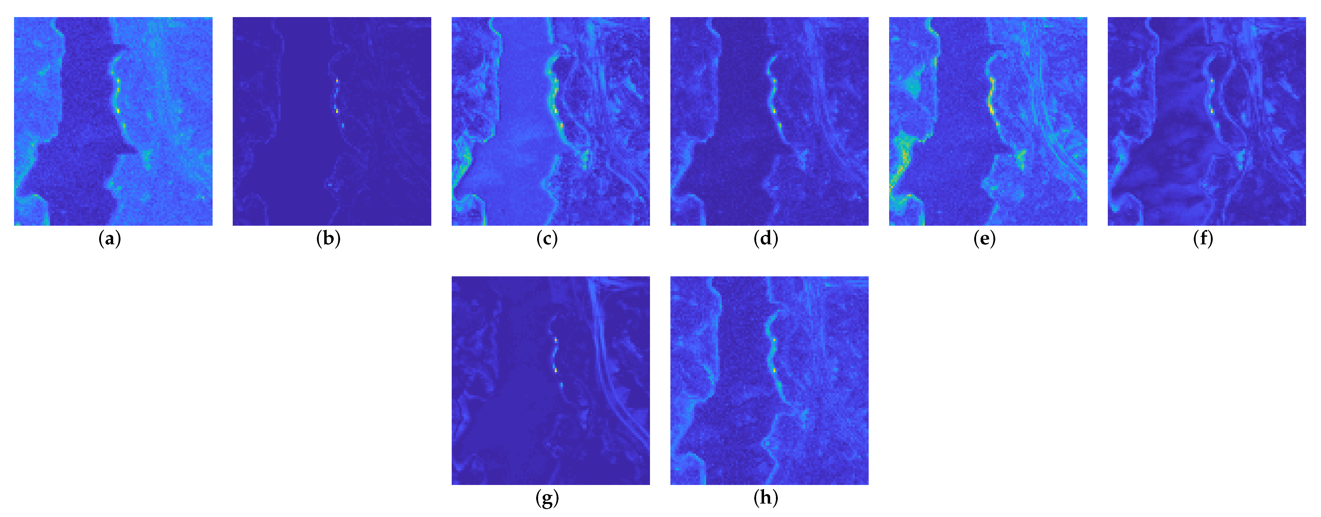
Figure 10 displays the detection results for Jasper Ridge data set. The total intensity of CBAD and RGAE is relatively low, causing unsatisfactory detection accuracy. The overall pixels of GRX hold high values, leading to a high false alarm rate. LSDM-MoG can detect most anomalies, but several background pixels are also highlighted. LRASR, AE, and LSMAD yield better results than LSDM-MoG. However, they all miss detecting plenty of anomalies. The PDRD has achieved better performance than other methods, and the results demonstrate the effectiveness of our proposed method.
ROC curves are shown in Figure 11c to evaluate the detection results qualitatively. As we can see, the ROC curve of our method lies in the upper-left corner of the image after the false alarm rate reaches 10 3 , and the detection probability quickly grows to a high level. When the false alarm rate is over 1 0 2 , the probability of detection is near to 1, which leads the performance among these methods to a great extent. As the detection probability of PDRD reaches 1, the largest of others is just 0.7, reflecting the superiority of the proposed PDRD algorithm.
Our method holds the best AUC scores, in line with the visualization of detection results and ROC curves. The effectiveness and superiority stem from the consideration of the intrinsic probability distribution of every single pixel. Consequently, the implicit structure of both anomalies and the background is well-recovered.

4.4. Parametric Analysis

In this part, we analyze how to set the optimal parameters for our PDRD algorithm. In addition, the optimal parameters of other methods are given in Table 3. For CBAD, R represents the quantization level. For LRASR, β and λ are the tradeoff parameters of lowrankness and sparsity, respectively. For LSMAD, r denotes the value of low rank. For LSDM-MoG, l 0 represents the initial rank, and K signifies the initial number of mixture Gaussian noise. For RGAE, λ denotes the tradeoff parameter of the graph regularization term.

4.4.1. Weight Parameter γ and Tradeoff Parameter β

The weight parameter γ determines the biased degree between the mean value and the standard deviation. After multiple experiments have been conducted, all of them reach the same conclusion that only if γ is set to 0 can our model reach powerful detection performance. Under the circumstance, the standard deviation acts as interference in our detection task, suggesting that only the mean value of the distribution influences the discrimination between the background and the anomalies. Hence, γ is set to 0 for all following experiments.
The tradeoff parameter β is used to balance the weight of reconstruction error and KL divergence term in the VAE loss function. The setting of β is significant in our experiment because the mutual independence of different dimensions depends on β . The experimental results further verify our aforementioned theoretical analysis. As we can observe from Figure 12a, the value of AUC grows as β increases in the preliminary stage. After reaching the maximum, it declines slowly from a general perspective. Specifically, with the rise of β , although the distribution in the latent space updates towards the direction that each dimension is mutually independent, the emphasis of the loss function in Equation (3) gradually tilts toward the KL divergence term, leading to the decline of the model reconstruction ability. The optimal parameter is acquired by trial and error, and the critical point is to unearth a balance between the reconstruction error and the KL divergence term.
The dimensionality k in the latent space is set to 30, 50, 40 for Pavia City, Gulfport, and Jasper Ridge data, respectively, and the local neighborhood ϵ is set to 23. Since the value of the KL divergence term is small, the range of the tradeoff parameter β we set is 1 , 10 , 50 , 100 , 200 , 500 , 1000 , 2000 , 5000 in the experiment. When β is equal to 1, the neural network represents the vanilla VAE. Moreover, the influence of β on three different hyperspectral data sets is not identical. The optimal setting values of β are 50, 500, and 50 for Pavia City, Gulfport, and Jasper Ridge data set, respectively.

4.4.2. Dimensionality k of Latent Variable

The distribution of latent variable signifies the intrinsic structure of original data in the feature space. The setting of k also deserves considerable attention. We can observe from Figure 12b that the value of AUC rises as k increases at the very beginning. After reaching the maximum, they keep at a high level or drop slightly. The phenomenon can be explained from the perspective of dimensional correlations. When k is too small, high correlations exist in different dimensions. As a result, low-dimensional probability representation in the latent space cannot extract sufficient information. On the contrary, if k is large enough or larger than the band number of HSI, various redundant dimensions will emerge.
Both β and ϵ remain unchanged when we optimize k. β is set to 50, 500, 50 for Pavia City, Gulfport, and Jasper Ridge data, respectively, and the local neighborhood ϵ is set to 23. Considering the actual band number of HSI, the range of parameter k is set to 1 , 2 , 5 , 10 , 20 , 30 , 40 , 50 , 100 , 150 , 200 . The experimental results indicate that the optimal setting values of k are 30, 50, and 40 for Pavia City, Gulfport, and Jasper Ridge data, respectively.

4.4.3. Chebyshev Neighborhood ϵ

The Chebyshev neighborhood ϵ determines the local information we utilize from the original hyperspectral image. Figure 12c demonstrates that when ϵ increases, the AUC score enhances at the very beginning. It declines as ϵ further increases after it reaches the maximum. When ϵ is small, the neighborhood only covers a small portion of adjacent areas. Therefore, the local information cannot be exploited thoroughly. When ϵ is too large, the adjacent areas contain many unexpected background categories. Moreover, the execution time increases quickly as ϵ grows.
The β and k are fixed when exploring the optimal setting of ϵ . β is set to 50, 500, 50 for Pavia City, Gulfport, and Jasper Ridge data, respectively. k is set to 30, 50, 40 for Pavia City, Gulfport, and Jasper Ridge data, respectively. The detection results reveal that the best values of ϵ we set are 23 for these three data sets.

4.4.4. Parameters of Neural Network

The learning rate α is crucial to the training procedure of a neural network. The appropriate setting value of α can accelerate the training process and promote the performance of the neural network. In our experiment, α is set to 1 0 4 for the three data sets.
The batch size of a neural network influences the learning accuracy and updating speed, and the optimal value is derived from trial and error with prior knowledge. It is set 32 for the three data sets.

4.5. Execution Time

In this part, we compare the execution time of these detectors. The experiments are conducted on a computer with a 64-bit Intel i7-8700 CPU of 3.2 GHz on Windows 10. To make a fair comparison, we implement all methods with CPU and the execution time includes the whole time of running all steps of the algorithm. Moreover, the execution time of these methods includes the training or optimizing process with the optimal parameters, but it does not include the trials of different parameters. The average execution time of the state-of-the-art methods for different data sets can be observed from Table 4. As we can see, GRX takes the least time among these methods. AE and RGAE are much slower as their training processes consume considerable time. Our proposed method can achieve good efficiency, which is just slower than GRX and CBAD.
Notably, our proposed method achieves high detection performance and obtains high computational efficiency simultaneously compared to other methods. Low computational cost and high detection accuracy make it possible to implement the method into practical applications.

4.6. Ablation Study

To evaluate the effect of each part on the final detection result, including probabilistic representation (PR), Chebyshev neighborhood (CN), and modified loss function (MLF), we have conducted an ablation study on three real hyperspectral data sets by eliminating the corresponding part, as Table 5 displays. In the first scenario, we try to eliminate the PR part. There are two strategies to accomplish the goal. We can replace the VAE with a regular AE and preserve other modules or eliminate the latent representations to conduct the experiments. The latter strategy means maintaining the VAE network and detecting the anomalies using reconstruction error, and we use the reconstruction error to detect the anomalies. Evidently, the AUC score decreases significantly for three data sets without the PR module, which indicates the validity of the PR module. With the removal of CN in the second scenario, we do not search the CN for each pixel. Instead, we exploit the global average expectation of all pixels to replace CN. the average AUC score is reduced by 1.8%, which manifests the usefulness of CN. When MLF is removed in the third scenario, the AUC score declines by 0.39%, embodying the effectiveness of MLF. From a comprehensive point of view, the average AUC scores of the models without PR, CN, and MLF are smaller than PDRD, which signifies the combination of Gaussian probabilistic representation, local Chevbyshev neighborhood, and the modification of loss function is effective for anomaly detection.

4.7. Discussion

To evaluate the effectiveness of the proposed method, we conducted our experiments on three data sets that are widely used in hyperspectral anomaly detection and compared the results with seven other detectors: GRX, CBAD, LRASR, LSMAD, LSDM-MoG, AE, RGAE.
In the proposed PDRD method, in order to fully explore the intrinsic characteristics of the original data, we exploit the VAE architecture that projects the image into the probabilistic feature space. A coefficient is added to the VAE loss function to balance the weight of reconstruction error and KL divergence. Consequently, we can obtain the disentangled features. After the network has been well trained, each training sample is transformed to a Gaussian distribution with a known mean value and a standard deviation. Moreover, we design the Chebyshev neighborhood that can leverage the spatial knowledge. We can finally acquire the anomaly detection map by computing the modified Wasserstein distance between the test pixel and its average expectation in the neighborhood. The proposed PDRD is different from the traditional VAE in two aspects. Firstly, the loss function is different. We add a parameter β to balance the weight of reconstruction error and KL divergence. Secondly, the detection strategy is different. Traditional VAE for hyperspectral anomaly detection inherits the neural network structure of the original VAE, and it exploits reconstruction error between the input image and output image to detect the anomalies. Our proposed PDRD leverage the probability representation in the latent space of the original data to accomplish the detection process.
For comparison, we employed ROC curves and AUC scores as the main criteria to comprehensively estimate the performance. As shown in Figure 11, the ROC curves of the proposed method always lie at the upper-left corner of the image, indicating that both the detection rate and false alarm rate are better than other methods. As illustrated in Table 2, it is evident that the detection power of the proposed method is better than that of other algorithms. According to these detection results and analysis, we conclude that the proposed method yields more excellent detection performance compared to other detectors.
Although our algorithm can achieve superior detection performance, several limitations still exist. The anomalies we mainly studied are targets in small regions whose spectral signature significantly differs from neighboring areas. The effectiveness of the proposed method on large-scale anomalies remains to be verified. The goal of our future work is to make the method algorithm universal.

5. Conclusions

In this paper, we propose a novel PDRD algorithm for hyperspectral anomaly detection. From a probabilistic perspective, we exploit multivariate Gaussian distributions to represent the whole image in the latent space. To take advantage of the spatial information, we introduce the ϵ Chebyshev neighborhood to estimate the local statistics. Finally, we compute the modified Wasserstein distance between the test pixel and its average expectation in the neighborhood. Experiments on three hyperspectral scenes demonstrate the accuracy and efficiency of our proposed method compared to the state-of-the-art detectors. However, it also needs to be highlighted that the proposed method may not be applicable for large-scale anomalies. In future work, we intend to combine the probability representation strategy with other neural networks to generalize the proposed model into more applications.

Author Contributions

All coauthors made significant contributions to the paper; S.Y. designed the research and analyzed the results; L.Z. and S.C. assisted in the prepared work and validation work; X.L. provided advice for the preparation and revision of the paper that improved the paper. All authors have read and agreed to the published version of the manuscript.

Funding

This work was funded in part by the National Nature Science Foundation of China under Grant 62171404, and in part by the Joint Fund of the Ministry of Education of China under Grant 6141A02022362. The authors would like to thank the editor and referees for their suggestions that improved the paper.

Institutional Review Board Statement

Not applicable.

Informed Consent Statement

Not applicable.

Data Availability Statement

The data used in this study are available at https://rslab.ut.ac.ir/data and http://xudongkang.weebly.com/data-sets.html (accessed on 24 May 2021).

Conflicts of Interest

The authors declare no conflict of interest.

References

  1. Cheng, T.; Wang, B. Graph and Total Variation Regularized Low-Rank Representation for Hyperspectral Anomaly Detection. IEEE Trans. Geosci. Remote Sens. 2020, 58, 391–406. [Google Scholar] [CrossRef]
  2. Landgrebe, D. Hyperspectral image data analysis. IEEE Signal Process. Mag. 2002, 19, 17–28. [Google Scholar] [CrossRef]
  3. Huang, Z.; Kang, X.; Li, S.; Hao, Q. Game Theory-Based Hyperspectral Anomaly Detection. IEEE Trans. Geosci. Remote Sens. 2020, 58, 2965–2976. [Google Scholar] [CrossRef]
  4. Bioucas-Dias, J.M.; Plaza, A.; Camps-Valls, G.; Scheunders, P.; Nasrabadi, N.; Chanussot, J. Hyperspectral Remote Sensing Data Analysis and Future Challenges. IEEE Geosci. Remote Sens. Mag. 2013, 1, 6–36. [Google Scholar] [CrossRef] [Green Version]
  5. Kruse, F.A.; Boardman, J.W.; Huntington, J.F. Comparison of airborne hyperspectral data and EO-1 Hyperion for mineral mapping. IEEE Trans. Geosci. Remote Sens. 2003, 41, 1388–1400. [Google Scholar] [CrossRef] [Green Version]
  6. Grohnfeldt, C.; Zhu, X.X.; Bamler, R. Jointly sparse fusion of hyperspectral and multispectral imagery. In Proceedings of the 2013 IEEE International Geoscience and Remote Sensing Symposium—IGARSS, Melbourne, VIC, Australia, 21–26 July 2013; pp. 4090–4093. [Google Scholar]
  7. Yu, S.; Li, X.; Zhao, L.; Wang, J. Hyperspectral Anomaly Detection Based on Low-Rank Representation Using Local Outlier Factor. IEEE Geosci. Remote Sens. Lett. 2021, 18, 1279–1283. [Google Scholar] [CrossRef]
  8. Nasrabadi, N.M. Hyperspectral Target Detection: An Overview of Current and Future Challenges. IEEE Signal Process. Mag. 2014, 31, 34–44. [Google Scholar] [CrossRef]
  9. Stein, D.W.J.; Beaven, S.G.; Hoff, L.E.; Winter, E.M.; Schaum, A.P.; Stocker, A.D. Anomaly detection from hyperspectral imagery. IEEE Signal Process. Mag. 2002, 19, 58–69. [Google Scholar] [CrossRef] [Green Version]
  10. Li, S.; Zhang, K.; Hao, Q.; Duan, P.; Kang, X. Hyperspectral Anomaly Detection With Multiscale Attribute and Edge-Preserving Filters. IEEE Geosci. Remote Sens. Lett. 2018, 15, 1605–1609. [Google Scholar] [CrossRef]
  11. Kingma, D.P.; Welling, M. Auto-encoding variational bayes. arXiv 2013, arXiv:1312.6114. [Google Scholar]
  12. Matteoli, S.; Diani, M.; Theiler, J. An Overview of Background Modeling for Detection of Targets and Anomalies in Hyperspectral Remotely Sensed Imagery. IEEE J. Sel. Top. Appl. Earth Obs. Remote Sens. 2014, 7, 2317–2336. [Google Scholar] [CrossRef]
  13. Ben Salem, M.; Ettabaa, K.S.; Hamdi, M.A. Anomaly detection in hyperspectral imagery: An overview. In Proceedings of the International Image Processing, Applications and Systems Conference, Hammamet, Tunisia, 5–7 November 2014; pp. 1–6. [Google Scholar]
  14. Li, J.; Zhang, H.; Zhang, L.; Ma, L. Hyperspectral Anomaly Detection by the Use of Background Joint Sparse Representation. IEEE J. Sel. Top. Appl. Earth Obs. Remote Sens. 2015, 8, 2523–2533. [Google Scholar] [CrossRef]
  15. Reed, I.S.; Yu, X. Adaptive multiple-band CFAR detection of an optical pattern with unknown spectral distribution. IEEE Trans. Acoust. Speech Signal Process. 1990, 38, 1760–1770. [Google Scholar] [CrossRef]
  16. Kwon, H.; Nasrabadi, N.M. Kernel RX-algorithm: A nonlinear anomaly detector for hyperspectral imagery. IEEE Trans. Geosci. Remote Sens. 2005, 43, 388–397. [Google Scholar] [CrossRef]
  17. Carlotto, M.J. A cluster-based approach for detecting human-made objects and changes in imagery. IEEE Trans. Geosci. Remote Sens. 2005, 43, 374–387. [Google Scholar] [CrossRef]
  18. Veracini, T.; Matteoli, S.; Diani, M.; Corsini, G. Fully Unsupervised Learning of Gaussian Mixtures for Anomaly Detection in Hyperspectral Imagery. In Proceedings of the 2009 Ninth International Conference on Intelligent Systems Design and Applications, Pisa, Italy, 30 November–2 December 2009; pp. 596–601. [Google Scholar]
  19. Matteoli, S.; Veracini, T.; Diani, M.; Corsini, G. Background Density Nonparametric Estimation With Data-Adaptive Bandwidths for the Detection of Anomalies in Multi-Hyperspectral Imagery. IEEE Geosci. Remote Sens. Lett. 2014, 11, 163–167. [Google Scholar] [CrossRef]
  20. Tidhar, G.A.; Rotman, S.R. Anomaly and target detection by means of nonparametric density estimation. In Proceedings of the SPIE, Baltimore, MD, USA, 23–24 April 2012; pp. 625–636. [Google Scholar]
  21. Banerjee, A.; Burlina, P.; Meth, R. Fast Hyperspectral Anomaly Detection via SVDD. In Proceedings of the 2007 IEEE International Conference on Image Processing, San Antonio, TX, USA, 16 September–19 October 2007; Volume 4, pp. IV-101–IV-104. [Google Scholar]
  22. Theiler, J.; Foy, B.R. EC-GLRT: Detecting Weak Plumes in Non–Gaussian Hyperspectral Clutter Using an Elliptically-Contoured Generalized Likelihood Ratio Test. In Proceedings of the IGARSS 2008—2008 IEEE International Geoscience and Remote Sensing Symposium, Boston, MA, USA, 7–11 July 2008; Volume 1, pp. I-221–I-224. [Google Scholar]
  23. Theiler, J.; Zimmer, B.; Ziemann, A. Closed-Form Detector for Solid Sub-Pixel Targets in Multivariate T-Distributed Background Clutter. In Proceedings of the IGARSS 2018—2018 IEEE International Geoscience and Remote Sensing Symposium, Valencia, Spain, 22–27 July 2018; pp. 2773–2776. [Google Scholar]
  24. Bengio, Y.; Courville, A.; Vincent, P. Representation Learning: A Review and New Perspectives. IEEE Trans. Pattern Anal. Mach. Intell. 2013, 45, 1798–1828. [Google Scholar] [CrossRef]
  25. Cai, J.; Candès, E.J.; Shen, Z. A Singular Value Thresholding Algorithm for Matrix Completion. SIAM J. Optim. 2010, 20, 1956–1982. [Google Scholar] [CrossRef]
  26. Li, W.; Du, Q. Collaborative Representation for Hyperspectral Anomaly Detection. IEEE Trans. Geosci. Remote Sens. 2015, 53, 1463–1474. [Google Scholar] [CrossRef]
  27. Sun, W.; Liu, C.; Li, J.; Lai, Y.K.; Li, W. Low-rank and sparse matrix decomposition-based anomaly detection for hyperspectral imagery. J. Appl. Remote Sens. 2014, 8, 1–18. [Google Scholar] [CrossRef]
  28. Wright, J.; Ganesh, A.; Rao, S.; Peng, Y.; Ma, Y. Robust Principal Component Analysis: Exact Recovery of Corrupted Low-Rank Matrices via Convex Optimization. In Proceedings of the 22th NIPS, Vancouver, BC, Canada, 7–10 December 2009; pp. 2080–2088. [Google Scholar]
  29. Xu, Y.; Wu, Z.; Li, J.; Plaza, A.; Wei, Z. Anomaly Detection in Hyperspectral Images Based on Low-Rank and Sparse Representation. IEEE Trans. Geosci. Remote Sens. 2016, 54, 1990–2000. [Google Scholar] [CrossRef]
  30. Liu, G.; Lin, Z.; Yan, S.; Sun, J.; Yu, Y.; Ma, Y. Robust Recovery of Subspace Structures by Low-Rank Representation. IEEE Trans. Pattern Anal. Mach. Intell. 2013, 35, 171–184. [Google Scholar] [CrossRef] [Green Version]
  31. Chen, Y.; Nasrabadi, N.M.; Tran, T.D. Simultaneous Joint Sparsity Model for Target Detection in Hyperspectral Imagery. IEEE Geosci. Remote Sens. Lett. 2011, 8, 676–680. [Google Scholar] [CrossRef]
  32. Zhang, Y.; Du, B.; Zhang, L.; Wang, S. A Low-Rank and Sparse Matrix Decomposition-Based Mahalanobis Distance Method for Hyperspectral Anomaly Detection. IEEE Trans. Geosci. Remote Sens. 2016, 54, 11376–11389. [Google Scholar] [CrossRef]
  33. Li, L.; Li, W.; Du, Q. Low-rank and sparse decomposition with mixture of gaussian for hyperspectral anomaly detection. IEEE Trans. Cybern. 2021, 51, 4363–4372. [Google Scholar] [CrossRef]
  34. Li, W.; Wu, G.; Du, Q. Transferred Deep Learning for Anomaly Detection in Hyperspectral Imagery. IEEE Geosci. Remote Sens. Lett. 2017, 14, 597–601. [Google Scholar] [CrossRef]
  35. Bati, E.; Alper Koz, A.; Aydin Alatan, A. Hyperspectral anomaly detection method based on auto-encoder. In Proceedings of the SPIE, Toulouse, France, 21–24 September 2015; pp. 220–226. [Google Scholar]
  36. Fan, G.; Ma, Y.; Mei, X.; Fan, F.; Huang, J.; Ma, J. Hyperspectral Anomaly Detection With Robust Graph Autoencoders. IEEE Trans. Geosci. Remote Sens. 2021; in press. [Google Scholar] [CrossRef]
  37. Lu, X.; Zhang, W.; Huang, J. Exploiting Embedding Manifold of Autoencoders for Hyperspectral Anomaly Detection. IEEE Trans. Geosci. Remote Sens. 2020, 58, 1527–1537. [Google Scholar] [CrossRef]
  38. An, J.; Sungzoon, C. Variational autoencoder based anomaly detection using reconstruction probability. Spec. Lect. IE 2015, 2, 1–18. [Google Scholar]
  39. Lei, J.; Fang, S.; Xie, W.; Li, Y.; Chang, C. Discriminative Reconstruction for Hyperspectral Anomaly Detection With Spectral Learning. IEEE Trans. Geosci. Remote Sens. 2020, 58, 7406–7417. [Google Scholar] [CrossRef]
  40. Kiran, B.R.; Thomas, D.M.; Parakkal, R. An overview of deep learning based methods for unsupervised and semi-supervised anomaly detection in videos. J. Imaging 2018, 4, 36. [Google Scholar] [CrossRef] [Green Version]
  41. Higgins, I.; Matthey, L.; Pal, A.; Burgess, C.; Glorot, X.; Botvinick, M.; Mohamed, S.; Lerchner, A. β-VAE: Learning Basic Visual Concepts with a Constrained Variational Framework. In Proceedings of the 5th ICLR, Toulon, France, 24–26 April 2017. [Google Scholar]
  42. Chen, R.T.Q.; Li, X.; Grosse, R.B.; Duvenaud, D.K. Isolating Sources of Disentanglement in Variational Autoencoders. In Proceedings of the 32th NeurIPS, Montreal, QC, Canada, 3–8 December 2018; pp. 2615–2625. [Google Scholar]
  43. Martin Arjovsky, S.C.; Bottou, L. Wasserstein Generative Adversarial Networks. In Proceedings of the 34th ICML, Sydney, NSW, Australia, 6–11 August 2017. [Google Scholar]
  44. Olkin, I.; Pukelsheim, F. The distance between two random vectors with given dispersion matrices. Linear Algebra Appl. 1982, 48, 257–263. [Google Scholar] [CrossRef] [Green Version]
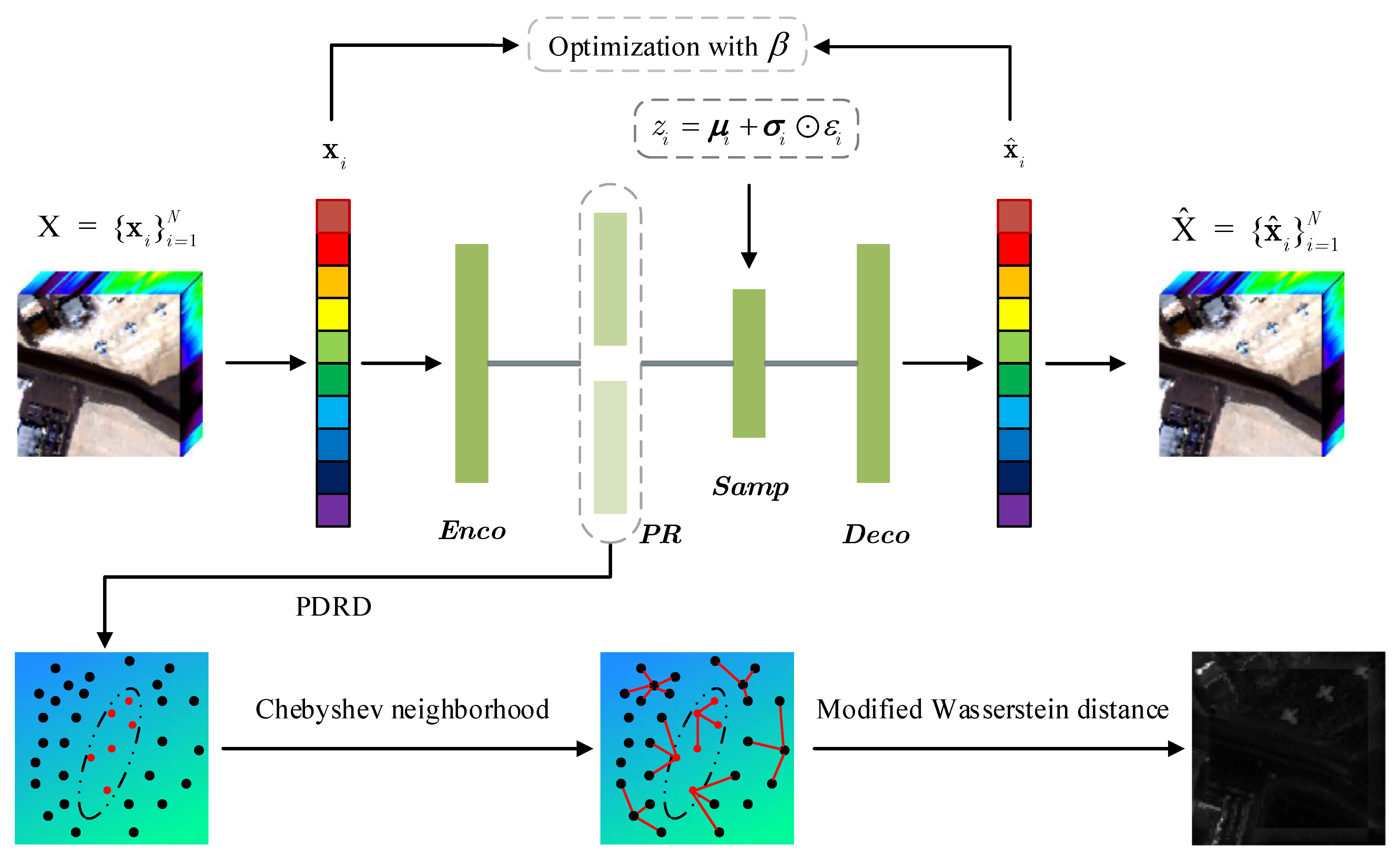
Figure 1. Framework of the proposed method. It mainly consists of three steps: (1) train the neural network and obtain the probability representation of each sample; (2) determine the Chebyshev neighborhood for each pixel; (3) obtain the detection map by computing the modified Wasserstein distance.
Remotesensing 14 00441 g001
Figure 2. The structure of VAE.
Remotesensing 14 00441 g002
Figure 3. The Chebyshev neighborhood when ϵ equals 1. The red pixels denote the test pixels. The green pixels represent the Chebyshev neighborhood.
Remotesensing 14 00441 g003
Figure 4. Calculation principles of different distances: (a) coordinate-wise distance; (b) Wasserstein distance.
Remotesensing 14 00441 g004
Figure 5. Descriptions of Pavia City data set: (a) pseudocolor image; (b) ground truth.
Remotesensing 14 00441 g005
Figure 6. Descriptions of Gulfport data set. (a) pseudocolor image; (b) ground truth.
Remotesensing 14 00441 g006
Figure 7. Descriptions of Jasper Ridge data set: (a) pseudocolor image; (b) ground truth.
Remotesensing 14 00441 g007
Figure 8. Two-dimensional maps of detection results by different algorithms for the Pavia City data set. (a) GRX; (b) CBAD; (c) LRASR; (d) LSMAD; (e) LSDM-MoG; (f) AE; (g) RGAE; (h) proposed.
Remotesensing 14 00441 g008
Figure 9. Two-dimensional maps of detection results by different algorithms for the Gulfport data set. (a) GRX; (b) CBAD; (c) LRASR; (d) LSMAD; (e) LSDM-MoG; (f) AE; (g) RGAE; (h) proposed.
Remotesensing 14 00441 g009
Figure 10. Two-dimensional maps of detection results by different algorithms for the Jasper Ridge data set. (a) GRX; (b) CBAD; (c) LRASR; (d) LSMAD; (e) LSDM-MoG; (f) AE; (g) RGAE; (h) proposed.
Remotesensing 14 00441 g010
Figure 11. Roc curves for different data sets: (a) Pavia City; (b) Gulfport; (c) Jasper Ridge.
Remotesensing 14 00441 g011
Figure 12. AUC values with the change of different parameters: (a) tradeoff parameter β ; (b) dimension parameter k; (c) neighborhood parameter ϵ .
Remotesensing 14 00441 g012
Table 1. Summarization of hyperspectral anomaly methods.
Method CategoryMethod CharacteristicsReferences
RX-basedComputing the Mahalanobis distance between the test pixel and background pixels[15,17]
Density and representation-basedDiscovering the spatial features and characterizing the distribution of anomalies and background pixels.[18,23,26]
Matrix decompositon-basedDecomposing the original data into a low-rank background component and a sparse anomaly component.[27,33]
Neural network-basedUsing reconstruction error of the original data to discriminate the anomalies from the background pixels.[34,39]
Table 2. AUC Scores for different data sets.
Data SetGRXCBADLRASRLSMADLSDM-MoGAERGAEProposed
Pavia City0.99060.99240.98240.99490.98070.98490.92920.9993
Gulfport0.95250.98000.95340.97430.98600.92990.89590.9919
Jasper Ridge0.87770.96340.94670.97410.93680.95790.82510.9968
Average0.94030.97860.96080.98110.96780.95760.88340.9960
Table 3. Optimal parameters of different detectors on three data sets.
Data SetCBADLRASRLSMADLSDM-MoGRGAEProposed
Pavia City R = 16 β = 0.1 , λ = 0.1 r = 4 l 0 = 12 , K = 4 λ = 0.001 β = 50 , k = 30 , ϵ = 23
Gulfport R = 8 β = 0.1 , λ = 0.1 r = 4 l 0 = 6 , K = 4 λ = 0.01 β = 500 , k = 50 , ϵ = 23
Jasper Ridge R = 16 β = 0.1 , λ = 0.1 r = 5 l 0 = 12 , K = 4 λ = 0.01 β = 50 , k = 40 , ϵ = 23
Table 4. Execution time (in seconds) for different data sets.
Data SetGRXCBADLRASRLSMADLSDM-MoGAERGAEProposed
Pavia City2.873.15132.9510.8339.4256.11145.333.12
Gulfport0.760.8823.048.4014.8836.5691.186.19
Jasper Ridge0.771.2627.2411.5414.3830.9395.173.6
Average1.471.7661.0810.2622.8941.20110.564.30
Table 5. AUC scores for component analysis.
ComponentPaviaGulfportJasper RidgeAverage
PDRD without PR (using reconstruction error of VAE)0.93500.64320.68120.7531
PDRD without PR (using AE)0.91300.91860.88550.9057
PDRD without CN0.97530.98680.97640.9795
PDRD without MLF0.99710.99060.99250.9934
PDRD0.99930.99190.99680.9960
Publisher’s Note: MDPI stays neutral with regard to jurisdictional claims in published maps and institutional affiliations.