Article

Validating the Crop Identification Capability of the Spectral Variance at Key Stages (SVKS) Computed via an Object Self-Reference Combined Algorithm

1
Key Laboratory of Digital Earth Science, Aerospace Information Research Institute, Chinese Academy of Sciences, Beijing 100094, China
2
University of Chinese Academy of Sciences, Beijing 100049, China
3
National Resource Center for Chinese Materia Medica, China Academy of Chinese Medical Sciences, Beijing 100700, China
4
College of Geology and Mining Engineering, Xinjiang University, Urumqi 830047, China
*
Author to whom correspondence should be addressed.
Remote Sens. 2022, 14(24), 6390; https://doi.org/10.3390/rs14246390
Submission received: 20 October 2022 / Revised: 9 December 2022 / Accepted: 12 December 2022 / Published: 17 December 2022
(This article belongs to the Special Issue Remote Sensing Applications in Vegetation Classification)

Abstract

:
Crop-distribution information constitutes the premise of precise management for crop cultivation. Euclidean distance and spectral angle mapper algorithms (ED and SAM) mostly use the spectral similarity and difference metric (SSDM) to determine the spectral variance associated with the spatial location for crop distribution acquisition. These methods are relatively insensitive to spectral shape or amplitude variation and must reconstruct a reference curve representing the entire class, possibly resulting in notable indeterminacy in the ultimate results. Few studies utilize these methods to compute the spectral variance associated with time and to define a new index for crop identification—namely, the spectral variance at key stages (SVKS)—even though this temporal spectral characteristic could be helpful for crop identification. To integrate the advantages of sensibility and avoid reconstructing the reference curve, an object self-reference combined algorithm comprising ED and SAM (CES) was proposed to compute SVKS. To objectively validate the crop-identification capability of SVKS-CES (SVKS computed via CES), SVKS-ED (SVKS computed via ED), SVKS-SAM (SVKS computed via SAM), and five spectral index (SI) types were selected for comparison in an example of maize identification. The results indicated that SVKS-CES ranges can characterize greater interclass spectral separability and attained better identification accuracy compared to other identification indexes. In particular, SVKS-CES2 provided the greatest interclass spectral separability and the best PA (92.73%), UA (100.00%), and OA (98.30%) in maize identification. Compared to the performance of the SI, SVKS attained greater interclass spectral separability, but more non-maize fields were incorrectly identified as maize fields via SVKS usage. Owning to the accuracy-improvement capability of SVKS-CES, the omission and commission errors were obviously reduced via the combined utilization of SVKS-CES and SI. The findings suggest that SVKS-CES application is expected to further spread in crop identification.

Graphical Abstract

1. Introduction

Crop production is the cornerstone of social development. According to the Statistical Yearbook 2021 of the Food and Agriculture Organization of the United Nations, about 1.6 billion ha of global croplands provided all cereals, vegetables, fruits, and other crop products to support peoples’ lives [1]. Such large-scale crop production and important food-security issues pose serious challenges to the precise management of crop cultivation. Remote sensing technology has become an effective means to provide accurate and low-cost services for crop cultivation [2,3,4,5], including early warning of pests and diseases [6,7], monitoring of nutrient and phenological phases [8,9], and irrigation–water estimations [10,11], etc. Spatial information on crop distribution is a prerequisite for specific analysis using remote sensing.
There are two main strategies for crop identification via remote sensing technology [12]. The first strategy considers the spectral characteristics of a single remote sensing image captured at a certain time; however, the optimal date can hardly be determined because crop fields exhibit similar spectral characteristics to those of other fields during the early and growing seasons [12,13]. The conspicuous phenomenon of different objects with the same spectral characteristics can produce more identification errors [14,15]. Therefore, the second strategy uses the spectral and temporal characteristics to characterize unique identification features including specific spectral values revealing phenological characteristics and the spectral variance reflecting growth variation [16,17,18,19]. For instance, Hu et al. [16] identified maize by using the differences in vegetation index (VI) values between maize and other fields over time. Shahrabi et al. [18] found that the temporal–spectral variance in the normalized difference vegetation index (NDVI) during the crop growing season could be used to compute an appropriate variable for maize identification.
The spectral similarity and difference metric (SSDM) is usually used to classify surface objects. This can characterize the interclass spectral separability or intraclass spectral variability [20,21,22,23]. There are four main SSDM computation methods: (1) the SSDM is computed based on the spectral distance, including the Euclidean distance algorithm (ED) [20,22] and the Jeffries–Matusita distance algorithm [23,24]; (2) the SSDM is computed using the spectral angle, including the spectral angle mapper algorithm (SAM) [25,26] and spectral gradient angle algorithm [27]; (3) the SSDM is computed via spectral information metrics, including the spectral information divergence algorithm [28]; and (4) the SSDM is computed considering the spectral correlation, including the spectral correlation measures algorithm [29]. Methods (1) and (2) are commonly used to identify crops involving remote sensing data, which assumes that the spectral characteristics are vectors in high-dimensional space, the dimensionality matches the number of spectral characteristics, and that the vector elements are the reflectance or VI [20,22,23]. Several researchers [20,21,22,23,30,31] directly computed the SSDM between a reference-class spectrum and other pixel spectra with different spatial locations using methods (1) and (2). According to the quantized values of SSDM, they mapped the large-scale spatial distribution of crops including maize, soybean, wheat, and paddy rice in China and the United States, utilizing a Moderate Resolution Imaging Spectroradiometer (MODIS) and Sentinel-1 and Sentinel-2 (S2) data. The above SSDM could be equivalent to the spectral variance associated with the spatial location. If two spectra of a single pixel on different dates were used for SSDM computation via methods (1) and (2), the obtained SSDM would be equivalent to the spectral variance associated with the time. As mentioned above, the temporal–spectral variance is helpful for crop identification [17,18], so we conjecture that the temporal–spectral variance computed via the SSDM computation methods has the same capability. However, there is little research that has validated this.
Our group intends to use ED and SAM for computing a new identification index; namely, the spectral variance at key stages (SVKS), in which the key stages cover phenological and land-use changes. Given that the computation processes of the ED and SAM are relatively uncomplicated, SVKS could become a type of universal and effective identification index similar to vegetation indexes for crop identification. Nevertheless, certain limitations of the ED and SAM cannot be neglected before application. The above temporal–spectral variance is directly related to the value of each element of the multidimensional vectors used in ED, while ED is insensitive to spectral shape variation [28]. Even if the variation in the spectral shape could be described, two curves with similar shapes but greatly different amplitudes could not be accurately captured with SAM [32]. Moreover, the reference curve selection and reconstruction problem cannot be ignored when using the algorithm to determine the spectral similarity and the difference between the target and reference [21,22]. Initially, a reference curve representing the entire class could be obtained by averaging multiple standard curves, resulting in a susceptibility of the reference curve to sequence shifts and dislocations, thus ultimately affecting the crop-identification accuracy [20]. Furthermore, the intraclass spectral variability cannot be represented by the reference curve [33] and researchers need to first determine the threshold range of each class [21,34]. Optimization methods for reference-curve reconstruction have been proposed [30]; for example, Li et al. [20], Shao et al. [21], and Mondal et al. [35] used the singular-value decomposition, Savitzky–Golay smoothing algorithm, asymmetric Gaussian smoothing algorithm, Fourier transformation and other methods for reference-curve reconstruction and found that spectral reconstruction could enhance the target identification accuracy. Nevertheless, the identification accuracy highly depends on the accuracy of the reconstructed reference curve.
To integrate the sensibility advantages, a combined algorithm comprising ED and SAM (CES) was applied in SVKS calculation, which can eliminate the limitations of using ED or SAM alone. Furthermore, we proposed an object self-reference method for ED and SAM usage to avoid reconstructing a reference curve representing the entire class. Such improvements would universalize and simplify the calculation of SVKS; however, the crop identification potential for CES is unknown. Therefore, three contents were designed to validate the crop identification capability of SVKS-CES (SVKS computed via CES): (1) analyzing the SVKS-CES performances for characterizing interclass spectral separability; (2) selecting maize and non-maize as examples and comparing the maize-identification accuracy of SVKS-CES to SVKS-ED (SVKS computed via ED), SVKS-SAM (SVKS computed via SAM), and five spectral index (SI) types; and (3) applying combined utilization of SVKS-CES and SI for classification and assessing the capability of accuracy improvement.

2. Materials and Methods

2.1. Study Area

In this study, we selected the agricultural area of Anqiu City, located in the eastern North China Plain within a geographical range of longitude 118°44′–119°40′E and latitude 36°05′–36°38′N (Figure 1). The North China Plain region is one of the most important agricultural hubs in China with a high population density and high demand for grain crops, producing approximately 23% of the national maize output [36,37]. As a typical agricultural county in the North China Plain, Anqiu City is the national demonstration base for the mechanization of major crop production. Arable land covering an area of 722.94 km2 occurs in the study area, which exhibits a temperate continental monsoon climate with a significant temperature variation between winter and summer. This area experiences an annual sunshine duration, rainfall, and average temperature of 2436 h, 631 mm, and 13 °C, respectively. Suitable climatic conditions and planting environments are provided for crops including maize, wheat, ginger, scallion, garlic, cherry, etc. Maize is one of the most widely planted crops in Anqiu City, commonly growing from June to October, after which it is rotated with winter wheat. During the maize-growing season, other open-air crops—mainly ginger, scallion, taro, nursery stock and fruit trees—are grown in this area. A calendar of these crops is shown in Figure 2.

2.2. Sentinel-2 Data and Preprocessing

Considering the availability of images and the spatial resolution of data in the study area, we collected S2 Multispectral Instrument data in this study. S2 Level-2A bottom-of-atmosphere (BOA) reflectance images were downloaded from the Google Earth Engine (GEE; https://earthengine.google.com (accessed on 26 April and 13 July 2022)) and Copernicus Open Access Hub (https://scihub.copernicus.eu (accessed on 2 and 5 November 2021)). According to the coverage of clouds and cloud shadows, five better-observed images acquired on 20 June, 10 July, 4 August, 8 September, and 13 October 2021 were selected. These images cover the growth stages of maize as well as the maize sowing and harvesting dates (Figure 2). Nine bands were used for calculation and analysis, including blue (band 2, B2), green (band 3, B3), red (band 4, B4), red-edge-1 (band 5 B5), red-edge-2 (band 6, B6), red-edge-3 (band 7, B7), near-infrared (NIR; band 8, B8), shortwave infrared-1 (SWIR-1; band 11, B11), and SWIR-2 (band 12, B12). The S2 data preprocessing workflow is shown in Figure 3. The spatial resolution of each image was resampled to 10 m in SNAP® software (https://step.esa.int/main/toolboxes/snap/ (accessed on 11 November 2021)) and GEE. Two tiles (50 SPF and 50 SQF) of image layers covering Anqiu City were stacked, clipped, and mosaicked in ENVI® software (https://www.l3harrisgeospatial.com/Software-Technology/ENVI (accessed on 27 July 2021)). Clouds and cloud shadows in each image were masked by using band QA60 and visual interpretation based on GEE and ENVI® software.

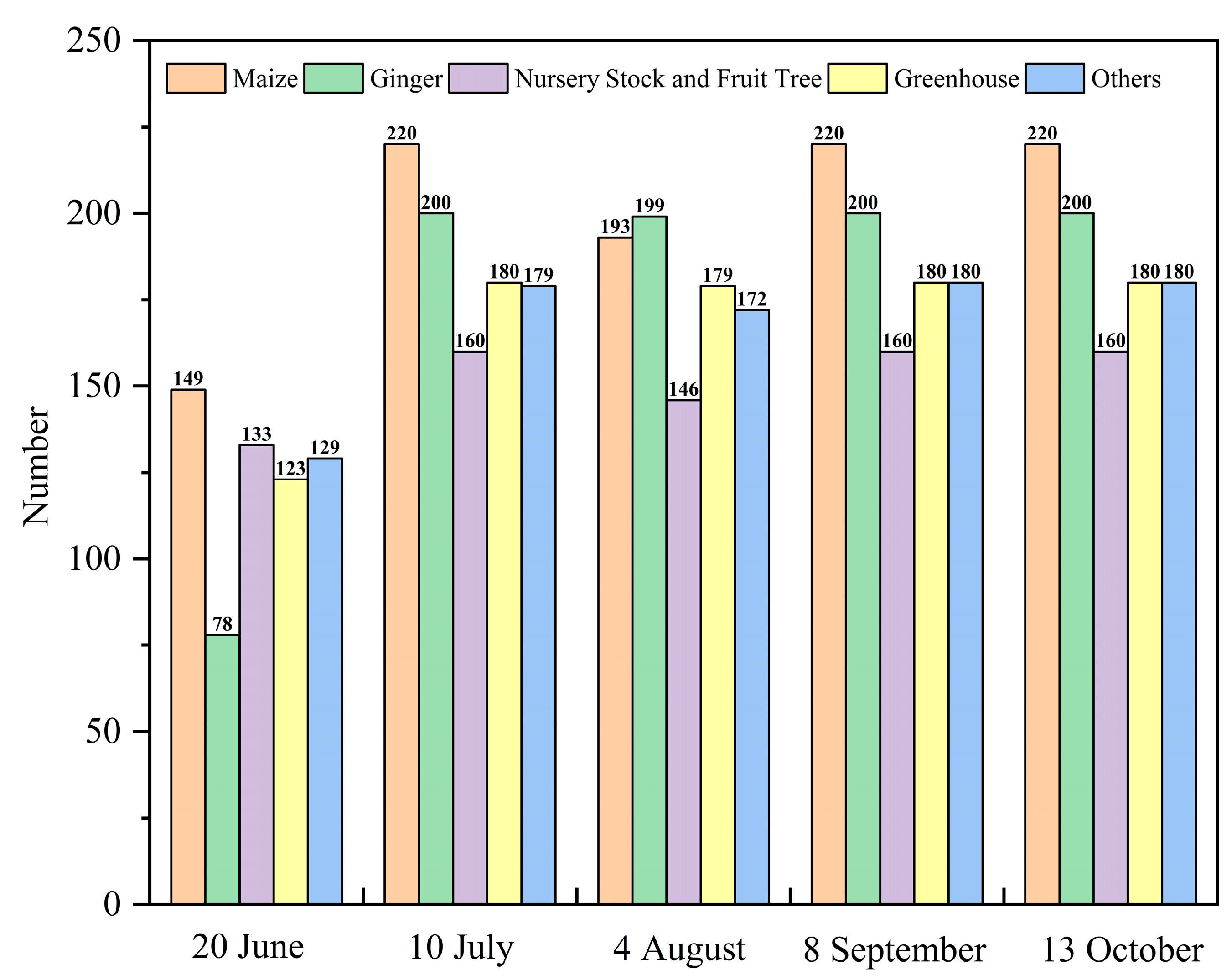
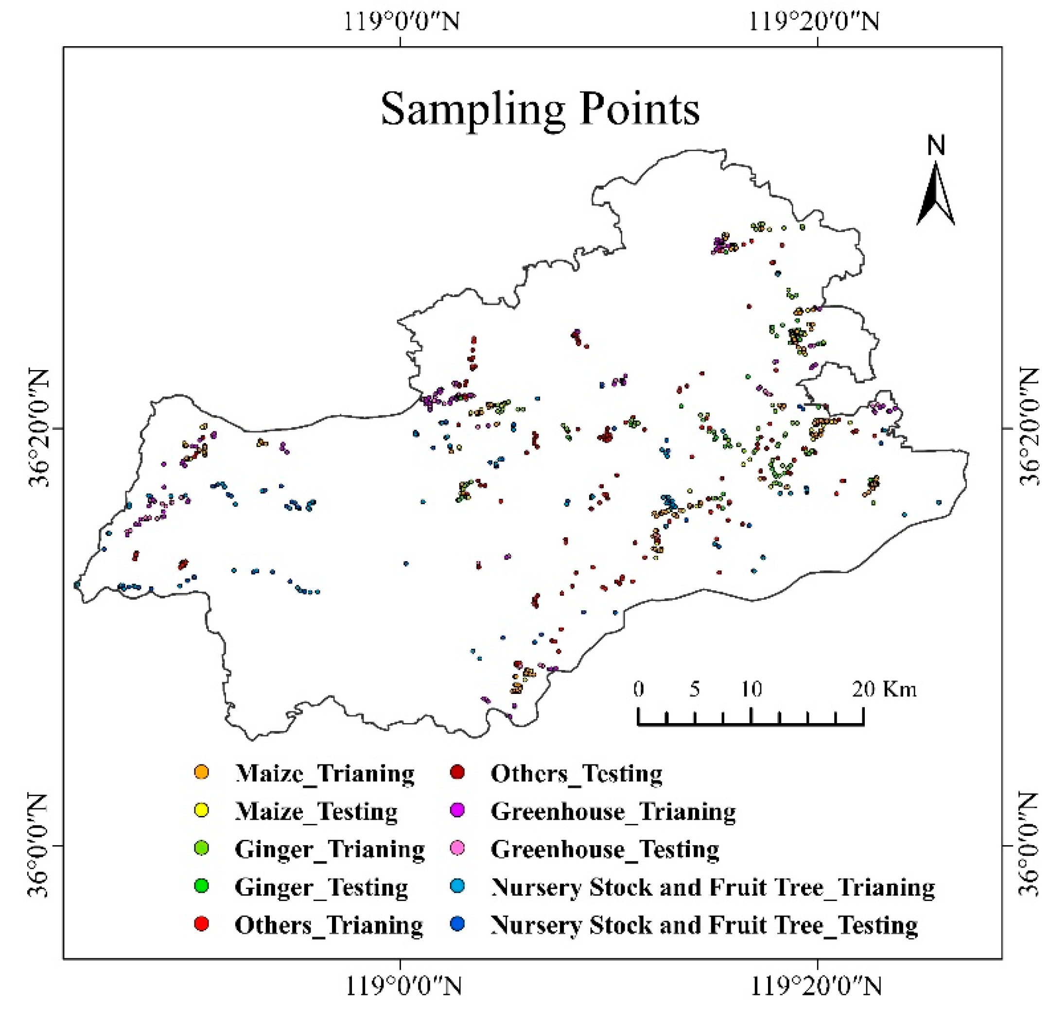
2.3. Field Observation

A field campaign was conducted in early August 2021 that covered the vigorous growth stage of maize. During the field campaign, 684 sampling points were recorded using a handheld Global Positioning System device with a positional error smaller than 2 m and 256 sampling points were established via visual interpretation of S2 images which were evenly distributed across the study area. We collected reference data including field types, geographic coordinates, photos, crop growth conditions, and phenological information. Considering the various field types, spectral characteristics, and crop phenology aspects, the sampling points could be divided into 220 maize sampling points, 200 ginger sampling points, 160 nursery stock and fruit tree sampling points, 180 greenhouse sampling points, and 180 other sampling points (including bare field, taro, scallion, and tobacco). The number of sampling points not covered by clouds or cloud shadows in each image is shown in Figure 4. Half of the sampling points were randomly selected for classifier training and the remaining points were employed for testing. The spatial distribution of the sampling points is shown in Figure 5.

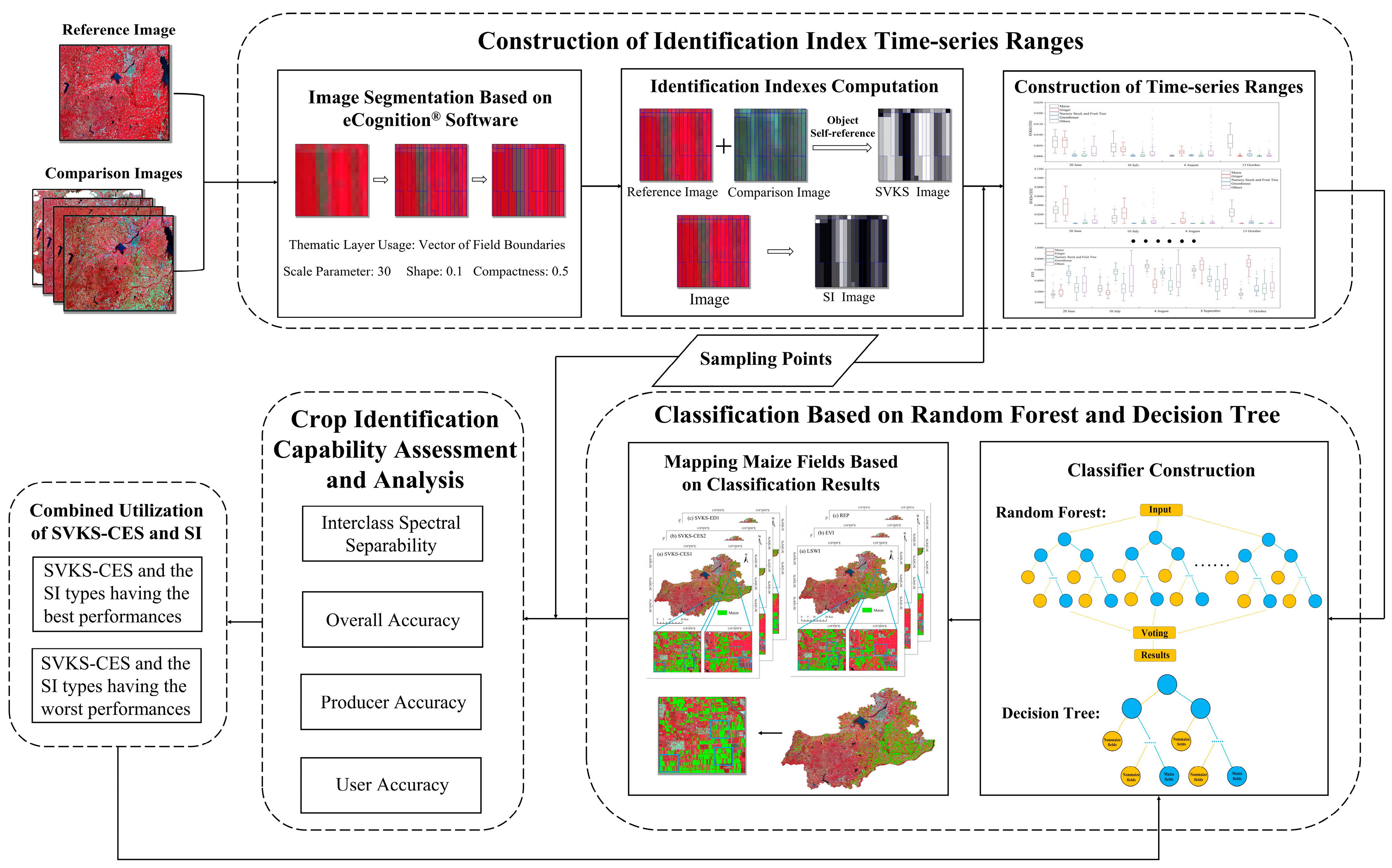
2.4. Experimental Design

To validate the crop-identification capability of SVKS-CES, the experiments were designed in three parts (the technical route is shown in Figure 6). The first part involved the construction of identification index time-series ranges. After pre-processing, the images were segmented into a spatially contiguous set of objects in eCognition® software and each object comprised a neighboring group of pixels with homogeneity or semantic significance. Following segmentation, SVKS-CES, SVKS-ED, SVKS-SAM, and five SI types were selected for computation via object self-reference. Additionally, SVKS and SI values were extracted at the sampling points for training to construct identification index time-series ranges for each class. The second part of the experiment entailed random forest (RF) and decision tree (DT) classifiers for classification; we constructed the RF and DT classifiers by using the time-series SVKS and SI values for machine learning, after which we used the constructed RF and DT classifiers to identify maize and non-maize. Finally, we mapped maize based on the classification results. The third part of the experiment involved accuracy assessment and analysis. We employed the performances of characterizing interclass spectral separability, overall accuracy (OA), producer accuracy (PA), and user accuracy (UA) to analyze and assess the crop identification capability of SVKS-CES. Finally, we selected the SI types exhibiting the best and worst performances to combine with the best SVKS-CES for classification and assessed the capability of accuracy improvement.

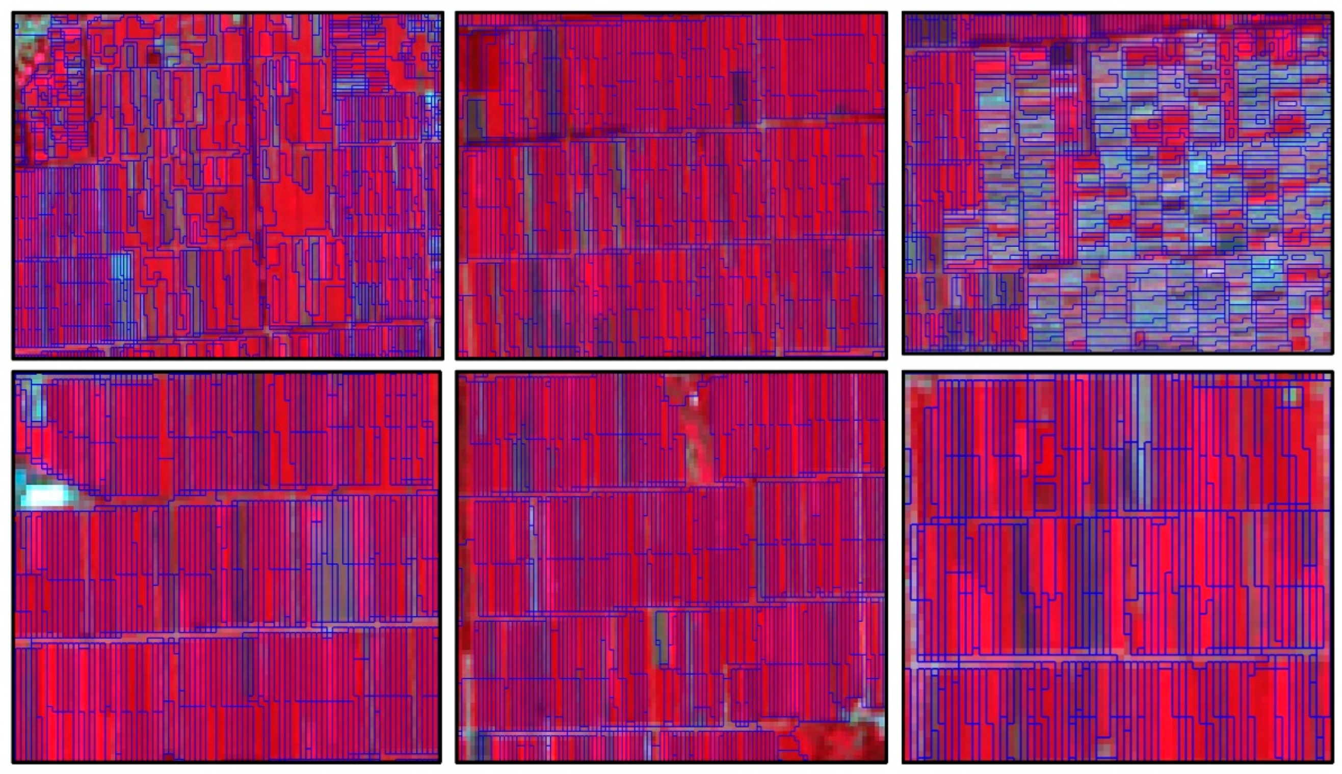
2.4.1. Image Segmentation

Intraclass spectral variability or interfield spectral variability could limit accuracy and result in a conspicuous salt-and-pepper effect when high-resolution data are subjected to pixel-based classification. Object-based classification could potentially overcome the inherent problems of pixel-based classification techniques [38]. Therefore, eCognition® software (https://geospatial.trimble.com/products-and-solutions/trimble-ecognition (accessed on 20 August 2021)) was utilized for image segmentation to perform object-based classification in this study [38,39]. Five parameters were needed in this segmentation algorithm: image layer weights, thematic layer usage, scale parameter, shape, and compactness. We set the image layer weights on 8 September to one and those on the other dates to zero, which guaranteed that the image segmentation process referred to the spectral and geometric characteristics of the image acquired on 8 September. The image acquired on 8 September was chosen as the reference image owing to the high image quality and abundant spectral information at the mature stage of maize. A vector of field boundaries (provided by GEOVIS Company Limited) covering the study area was input as the thematic layer, guaranteeing that the reference image acquired on 8 September was segmented along the vector of field boundaries. Any two parameters (scale parameter, shape, and compactness) were maintained as constants while the remaining parameter was varied to determine the appropriate input value (the test combinations are listed in Table 1), thus guaranteeing the prevention of undersegmentation and oversegmentation. Finally, we selected scale parameter, shape, and compactness values of 30, 0.1, and 0.5, respectively. The selection of these parameters was performed to avoid undersegmentation and excessive oversegmentation. We only needed to ensure that the pixels in each object belonged to the same class, so moderate oversegmentation was permitted. The image segmentation result is shown in Figure 7.

2.4.2. Computation of the Identification Indexes

As temporal–spectral variance can be used in crop identification [18], SVKS was proposed to indicate the spectral characteristic of each class in this study. We used ED and SAM as well as a combined ED with SAM to calculate SVKS through object self-reference, as is expressed in Equations (1)–(3). Instead of exhaustive combinations, two-band combinations were selected for SVKS calculation on 20 June, 10 July, 4 August, and 13 October as validation of the potential of SVKS-CES for crop identification was the main purpose of this study. The band combinations are summarized in Table 2.
SVKS-CES = i = 1 n OS i OC i 2 · 1 i = 1 n OS i · OC i / i = 1 n OS i 2 · i = 1 n OC i 2
SVKS-ED = i = 1 n OS i OC i 2
SVKS-SAM = i = 1 n OS i · OC i / i = 1 n OS i 2 · i = 1 n OC i 2
where OSi denotes the BOA reflectance of the object within the i-th band in the reference image acquired on 8 September, OCi denotes the BOA reflectance of the object within the i-th band in the image at the comparison time, and n denotes the number of bands in the spectrum curve.
To evaluate the performance of SVKS, the enhanced vegetation index (EVI), NDVI, green-normalized difference vegetation index (GNDVI), land surface water index (LSWI), and red-edge position (REP) were calculated based on five images. The NDVI and EVI can represent crop growth with a sufficient sensitivity; NDVI performs better during lower-biomass periods and EVI performs better during higher-biomass periods [40]. The GNDVI has been verified as an effective index for representing the content of photosynthetic pigments [40]. The LSWI is a suitable indicator of the vegetation moisture content and can facilitate crop identification during the growing season [13]. In addition, REP contributes to crop identification [13]. These indexes can be obtained as follows:
EVI = 2.5 · ρ B 8 ρ B 4 ρ B 8 + 6 · ρ B 4 7 . 5 · ρ B 2 + 1
NDVI = ρ B 8 ρ B 4 ρ B 8 + ρ B 4
GNDVI = ρ B 8 ρ B 3 ρ B 8 + ρ B 3
LSWI = ρ B 8 ρ B 11 ρ B 8 + ρ B 11
REP = 705 + 35 · 0 . 5 · ρ B 7 + ρ B 4 ρ B 5 ρ B 6 ρ B 5
where ρB2, ρB3, ρB4, ρB5, ρB6, ρB7, ρB8, and ρB11 denote the BOA reflectance of the object within B2, B3, B4, B5, B6, B7, B8, B11, and B12, respectively.

2.4.3. Random Forest and Decision Tree-Based Classification

In this study, we selected RF and DT classifiers for classification in eCognition® software owning to their mature remote sensing applications. RF is an assembler machine learning program which can handle big data efficiently and qualify outliers and overfitting [41,42]. DT is similar, with a hierarchy composed of a root node including all samples, a node separator containing decision rules, and the end of the leaf node representing desired classes [43]. Some non-parametric classification and decision tree or CART (classification and regression trees) can form an RF [43]. There are six parameters required in an RF classifier: depth, minimum sample count, maximum categories, active variables, maximum tree number, and forest accuracy. Additionally, a DT classifier needs four parameters: depth, minimum sample count, maximum categories, and cross validation folds. Given that the purpose of this study is not to improve the classifiers, we set all the above-listed parameters as software default values (listed in Table 3). RF and DT classifiers were trained and applied via machine learning with time-series identification indexes.

2.4.4. Accuracy Computation

The predictions for each class derived from RF and DT classification were compared to 470 sampling points for testing. The results are presented in three confusion matrices (Section 3.2, Section 3.3 and Section 3.4) considering OA, PA, and UA. To objectively assess and analyze the crop identification capability of SVKS-CSE, we compared the SVKS-CSE performance to those of other identification indexes. OA, PA, and UA can be calculated with Equations (7)–(9), respectively.
OA = TP + TN N
PA = TP TP + FN
UA = TP TP + FP
where TP and FN denote the number of sampling points employed for testing correctly identified as maize fields and the number of sampling points employed for testing incorrectly identified as non-maize fields (including ginger, nursery stock and fruit tree, greenhouse, and others), respectively. Moreover, TN and FP denote the number of sampling points employed for testing correctly identified as non-maize and the number of sampling points employed for testing incorrectly identified as maize, respectively, and N denotes the total number of sampling points considered for testing.

3. Results

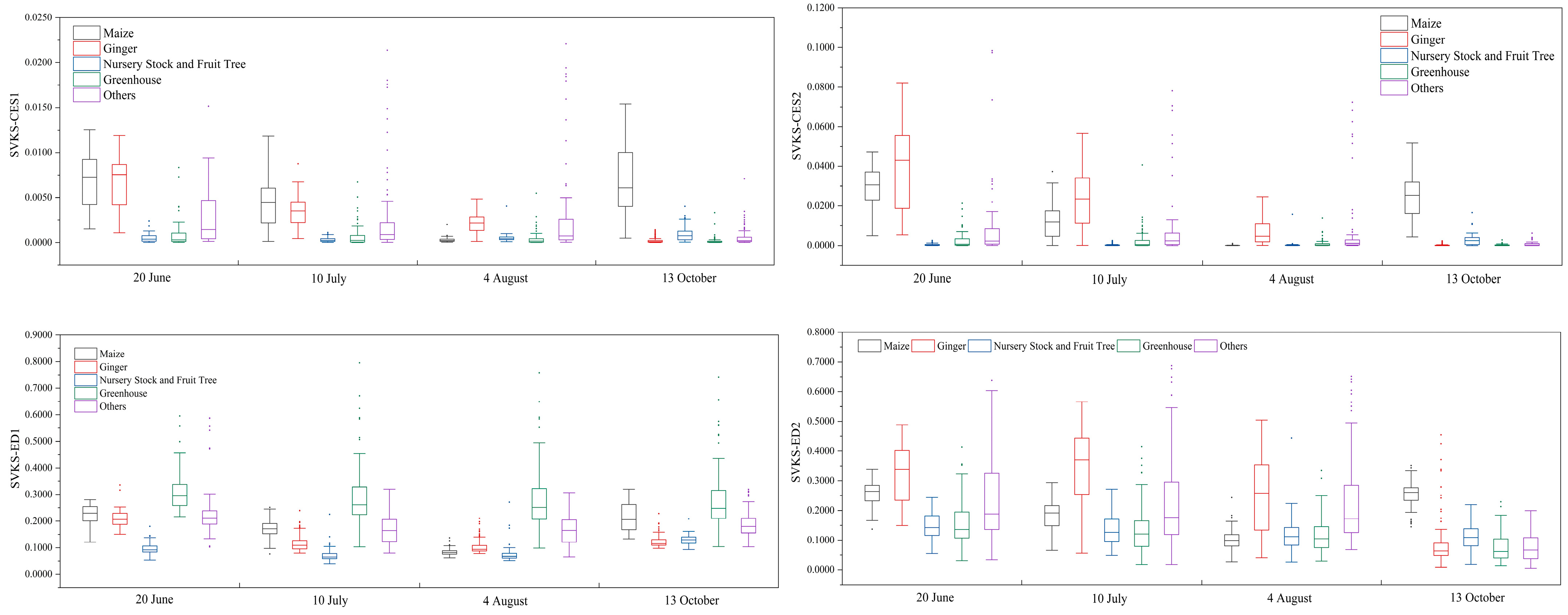
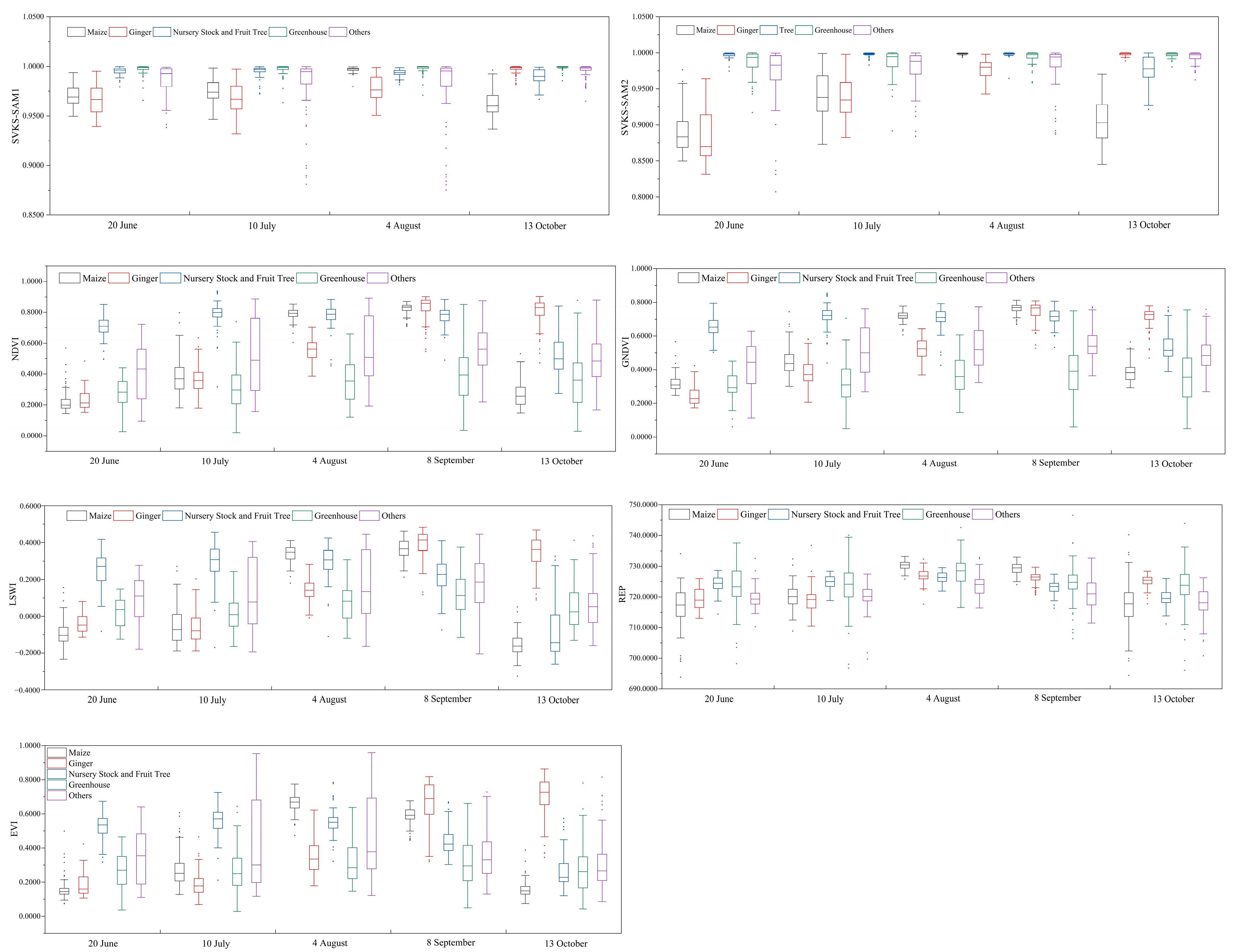
3.1. Feature Analysis of the Identification Index Time-Series Ranges

The time-series ranges of each identification index are shown in the boxplots below (Figure 8). The upper and lower bounds of each range (the minimum and maximum range values can be calculated with Equations (12) and (13), respectively) in the boxplots determine the range of SVKS or SI for a given class. An overlap of the interclass ranges of SVKS or SI could indicate that the same values of SVKS or SI occur in different classes, which could produce identification errors. Therefore, we must focus on the non-overlapping interclass ranges of SVKS and SI which could provide better interclass spectral separability. There was no overlap between the ranges of maize and nursery stock and fruit tree for SVKS-CES1 (SVKS computed via CES with band combination 1), SVKS-CES2 (SVKS computed via CES with band combination 2), SVKS-ED2 (SVKS computed via ED with band combination 2), EVI, GNDVI, LSWI, and NDVI on 20 June and NDVI on 10 July. The ranges of maize did not overlap the ranges of ginger for SVKS-CES1, SVKS-CES2, SVKS-ED2, SVKS-SAM1 (SVKS computed via SAM with band combination 1), SVKS-SAM2 (SVKS computed via SAM with band combination 2), EVI, GNDVI, LSWI, and NDVI, the ranges of greenhouse for SVKS-CES1, SVKS-CES2, SVKS-ED2, SVKS-SAM1, and SVKS-SAM2, as well as the ranges of others for SVKS-CES2, SVKS-SAM1 and SVKS-SAM1 on 13 October. Additionally, the ranges of maize did not overlap the ginger and greenhouse ranges, including GNDVI and NDVI, on 4 August. There was less or no overlap between ginger, nursery stock, and fruit tree ranges for SVKS-CES2, SVKS-SAM2, NDVI, GNDVI, and EVI on 20 June and 10 July, as well as SVKS-ED1 (SVKS computed via SAM with band combination 1) and LSWI on 20 June. The ranges of ginger overlapped less with the greenhouse ranges for SVKS-CES2 and SVKS-SAM2. There was less or no overlap between greenhouse, nursery stock, and fruit tree ranges for NDVI and GNDVI on 20 June, 10 July and 4 August. However, the ranges of maize overlapped with the ranges of others for all SI types and also overlapped with the non-maize ranges for REP at all times. In conclusion, SVKS-CES2 ranges provide the least overlap between different crops, which characterizes the greatest interclass spectral separability. Furthermore, we found that band increase resulted in a conspicuous intraclass spectral variability phenomenon based on the wider ranges of SVKS.
Maximum = 2 . 5 Q 3 1 . 5 Q 1
Minimum = 2 . 5 Q 1 1 . 5 Q 3
where Q1 and Q3 are the first and third quartiles, respectively.

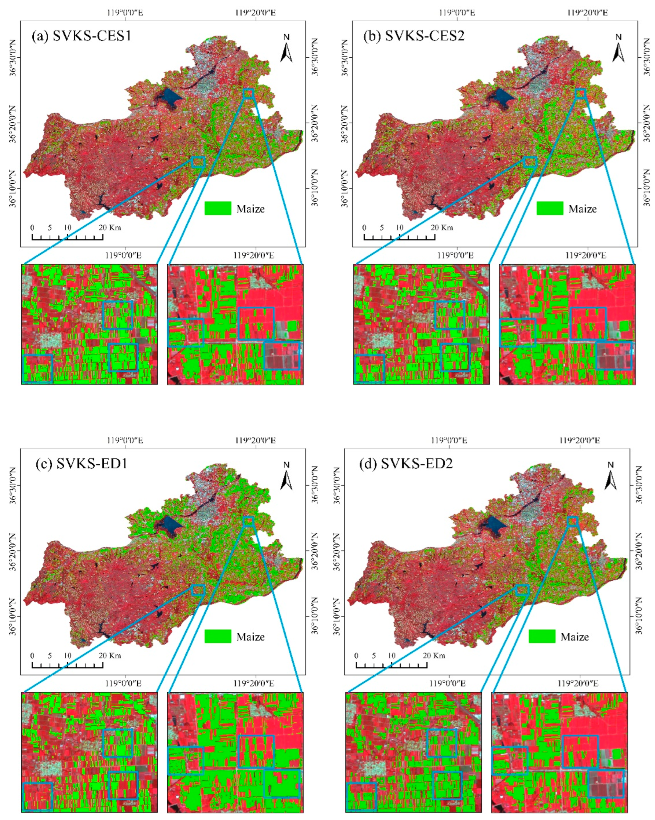
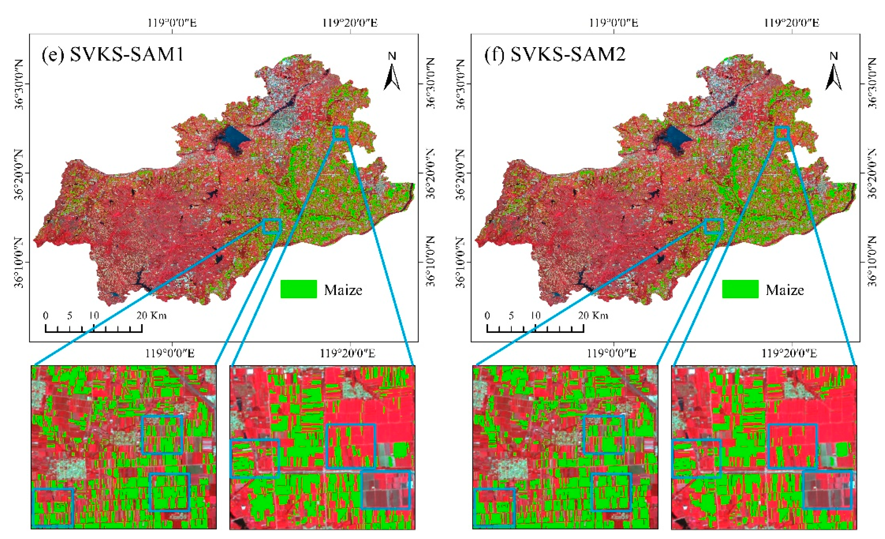
3.2. Maize Identification Based on a Single SVKS Type

Here, a single SVKS type was used to train RF and DT classifiers for classification. In terms of the mapping results, we found that maize was mainly distributed in the plains of central and eastern Anqiu City (Figure 9), which is consistent with the actual situation. The SVKS map could produce homogeneous fields with clear boundaries and few salt-and-pepper effects (Figure 9a–f). The different SVKS types achieved various performance levels in maize identification. The confusion matrices indicating the identification accuracy of each SVKS type are provided in Table 4. More bands involved in SVKS calculation seem to upgrade the identification accuracy, regardless of whether the classifier or SVKS calculation method was used. For example, the UA, PA, and OA of SVKS-CES1 were lower than those of SVKS-CES2, and the UA and OA of SVKS-ED2 were higher than those of SVKS-ED1. We found that the identification accuracy of SVKS-CES performed better than that of SVKS-ED and SAM. In particular, the accuracy of SVKS-CES2 indicated the highest PA, UA, and OA. According to the classifier comparison, an RT can slightly improve the performance of SVKS-CSE. Owing to the fewer omission errors (objects where the identification result was non-maize but the true result was maize) and commission errors (objects where the identification result was maize but the true result was non-maize) in maize-identification results, SVKS-CES can increase PA, UA, and OA by 0–9.09%, 1.94–45.55%, and 0.43–19.78%, respectively, compared to SVKS-ED and SAM.

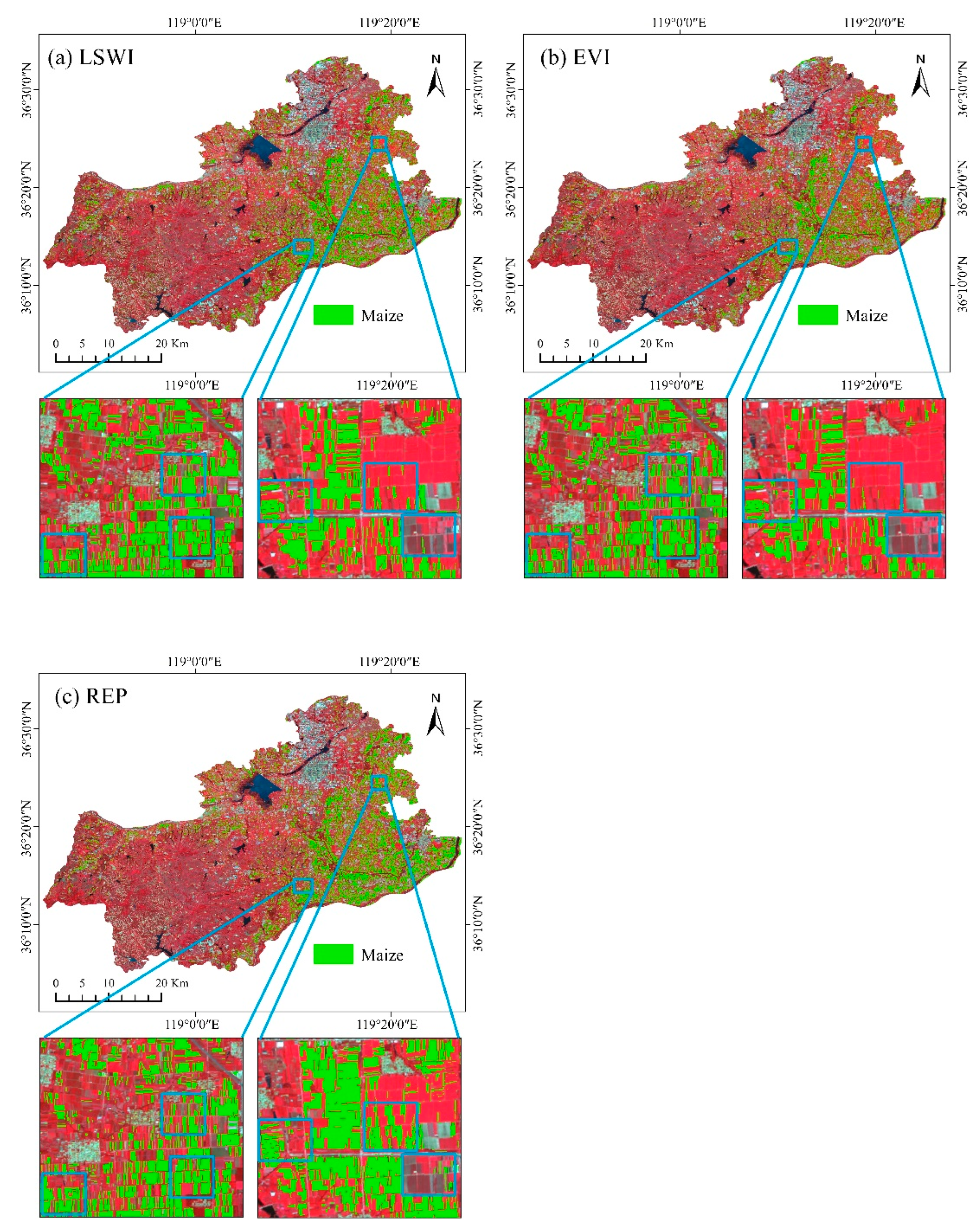
3.3. Maize Identification Based on a Single SI Type

We conducted the same experiments as above (Section 3.2) for the five SI types to assess their individual performance in terms of maize identification. In the SI map, some fields were inhomogeneous with unobvious boundaries (Figure 10a–c). The confusion matrices indicating the identification accuracy of each SI type are provided in Table 5. There were significant differences in the performance among the various SI and classifier types. Even if the accuracy of EVI, NDVI, GNDVI, and LSWI demonstrated that the OA value exceeded 91% and the UA value exceeded 82%, REP attained the lowest OA (85.53%) and UA (65.91%) from DT-based classification which resulted from the larger number of incorrectly identified fields. The LSWI was the best SI owing to its exhibition of steadily better performance, regardless of whether the classifier was used. Although all the SI types except REP performed well in excluding non-maize (higher UA values), they produced larger commission errors in maize extraction.

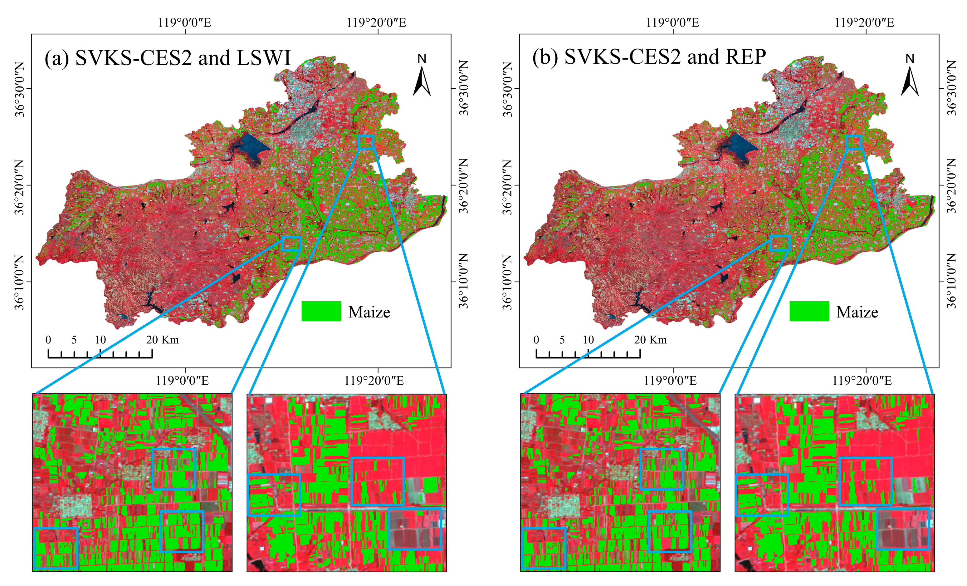
3.4. Crop Identification Capability Analysis and Assessment

Comparing the performance of SVKS to SI, we found that SVKS-CES was the best identification index for characterizing the best interclass spectral separability and providing the best classification accuracy. To further validate the crop-identification capability of SVKS-CES, we selected LSWI and REP, respectively having the best and worst performances, and time-series SVKS-CES2 (having the best performances) was combined with LSWI and REP to train the RF classifier for maize identification. The confusion matrices indicating the identification accuracy of each combined utilization type are provided in Table 6. We found that the addition of SVKS-CES2 can obviously improve the identification accuracy using a single LSWI or REP. Owing to the decrease in omission errors and commission errors (Figure 11), the PA, UA, and OA maximums increased by 7.27%, 15.69% and 5.11%, respectively.

4. Discussions

In this study, an object self-reference combined algorithm comprising ED and SAM (CES) was proposed to calculate SVKS and the crop-identification capability of SVKS-CES had been validated and discussed. Regarding the unique features characterized by the identification indexes, we found that SVKS-CES2 ranges of different classes had the least overlap compared to that of other identification indexes, which characterized that SVKS-CES2 ranges can provide the best interclass spectral separability. When selecting the feature for classifier training before classification, good interclass spectral separability is a useful indicator for determining which index has better crop-identification potential. For example, SVKS-CES2 and REP provide the best and worst interclass spectral separability and attained the best and worst identification accuracy, respectively. Regarding the SVKS performance in maize identification, the OA of SVKS-CES exceeded 96%, the PA of SVKS-CES exceeded 90%, and the UA exceeded 96%. Compared to the accuracy of other SVKS types, SVKS-CES exhibited the highest OA and UA which integrated the advantages of the highest PA of SVKS-ED and the higher UA of SVKS-SAM. The reason for these results could be that more key information benefiting identification is provided by the red-edge and NIR bands [13,44,45]. It is helpful for SVKS to characterize the intraclass spectral variability and improve identification accuracy by increasing the number of bands in SVKS calculation. The number of bands could not exhibit the same increasing relationship as that of the SVKS accuracy as redundant bands could mask the distinction between classes and aggravate the typical phenomenon of different objects with the same spectral characteristics [16,46]. Compared to the accuracy of SVKS-CES2, SVKS-CES1 exhibited a lower PA, UA, and OA because the similar interclass spectral variance values attributed to similar visible-light absorption and chlorophyll-reflection levels could reduce the spectral separability between maize and non-maize fields [12].
According to the temporal characteristics of SVKS, SVKS-CES could favorably distinguish maize from non-maize on 20 June and 13 October. We found that the SVKS-CES values of maize deviated from zero on 20 June, while those of nursery stock and fruit trees exhibited the opposite phenomenon as the spectrum curve of maize was similar to that of bare soil before the seedling stage but significantly different from that at the mature stage, while no considerable spectral variation occurred in nursery stock and fruit tree fields owing to the absence of senescence and harvesting. Furthermore, the SVKS-CES values of maize deviated from zero on 13 October while those of ginger, greenhouse, and others exhibited the opposite phenomenon due to the spectrum curve of maize being similar to that of bare soil or maize straw after the harvest. No considerable variation in the spectrum curve occurred in the ginger, greenhouse, and other fields owing to the absence of sowing or harvesting.
Compared to the performance of SI (the average PA, UA, and OA were 79.73%, 91.23% and 93.15%, respectively), we found that the average PA (89.39%) and OA (93.94) of SVKS were higher because of the better interclass spectral separability that occurred in SVKS ranges. However, more non-maize fields were incorrectly identified as maize fields using SVKS (the average UA was 88.94%), which indicates that interclass spectral variance similarity produced larger commission errors. The different performance levels of the various SI types indicated a great variation in identification results. Therefore, higher accuracy can be obtained by combining SVKS and certain SI types in maize identification [12]. To assess the capability of accuracy improvement, SVKS-CES2 was selected to be combined with LSWI and REP for classification. The results showed that the addition of SVKS-CES2 can obviously reduce the omission and commission errors from LSWI- or REP-based classification, which illustrated that SVKS-CES provides greater application potential in crop identification. This is a promotion for feature selection before classifier training. We also applied various SVKS-CES and SI combinations to identify glycyrrhiza uralensis Fisch. plants and achieved satisfactory results.
The following limitations of this study should be noted, which represent future directions to further improve the proposed identification method: first, only five images were selected at the key stages of maize, while some features benefiting identification may have been ignored due to the large time interval. Second, missing data in certain regions due to clouds and cloud shadows may lead to uncertainties in the identification results. In particular, this identification method cannot be used in regions of the reference image with missing data. Third, the importance of each band for SVKS-CES identification accuracy was not evaluated in this study.

5. Conclusions

SVKS computed via the object self-reference combined algorithm provides a new useful index for crop identification. Compared to the performances of SVKS-ED, SVKS-SAM, and SI, SVKS-CES characterizes greater interclass spectral separability and attained better identification accuracy, which demonstrates that SVKS-CES integrated the advantages of SVKS-ED and SVKS-SAM. The crop-identification capability assessment of each index illustrated that SVKS-CES2 provided the greatest interclass spectral separability and the best PA (92.73%), UA (100.00%), and OA (98.30%) in maize identification. A performance comparison of SVKS to SI confirmed that the ranges of SVKS provided greater interclass spectral separability. However, more non-maize fields were incorrectly identified as maize fields via SVKS usage, which indicates that interclass spectral variance similarity could produce larger commission errors. Although the different performance levels of the various SI types indicated great variation in identification results, the combined utilization of SVKS-CES2 and SI can obviously reduce the omission and commission errors from the SI-based classification.

Author Contributions

Conceptualization, H.Z. and J.M.; methodology, H.Z. and J.M.; formal analysis, H.Z.; resources, H.Z., J.M., T.S., X.Z. and Y.W.; writing—original draft preparation, H.Z.; writing—reviewing and editing, H.Z., J.M., T.S., X.Z., Y.W., X.L., Z.L. and X.Y.; funding acquisition, J.M., T.S. and X.Z.; visualization, H.Z. and J.M.; supervision, J.M. All authors have read and agreed to the published version of the manuscript.

Funding

This study was supported by the Innovation Fund of the China Academy of Chinese Medical Sciences (Grants No. CI2021A03901 and CI2021A03902) and the National Natural Science Foundation of China (Project No. 41871261).

Data Availability Statement

The authors do not have permission to share data.

Acknowledgments

We gratefully thank GEOVIS Company Limited for providing the basic local materials of Anqiu City. We are also especially thankful to the local management committee of Anqiu City for providing help during the field campaign.

Conflicts of Interest

The authors declare no conflict of interest.

References

  1. Food and Agriculture Organization of the United Nations. Statistical Yearbook. 2021. Available online: https://www.fao.org/3/cb4477en/online/cb4477en.html (accessed on 31 May 2022).
  2. Wang, P.; Wu, D.; Yang, J.; Ma, Y.; Feng, R.; Huo, Z. Summer maize growth under different precipitation years in the Huang-Huai-Hai plain of China. Agric. For. Meteorol. 2020, 285–286, 107927. [Google Scholar] [CrossRef]
  3. Wang, Y.; Fang, S.; Zhao, L.; Huang, X.; Jiang, X. Parcel-based summer maize mapping and phenology estimation combined using Sentinel-2 and time series Sentinel-1 data. Int. J. Appl. Earth Obs. Geoinf. 2022, 108, 102720. [Google Scholar] [CrossRef]
  4. Xun, L.; Wang, P.; Li, L.; Wang, L.; Kong, Q. Identifying crop planting areas using Fourier-transformed feature of time series MODIS leaf area index and sparse-representation-based classification in the North China plain. Int. J. Remote Sens. 2019, 40, 2034–2052. [Google Scholar] [CrossRef]
  5. Zhang, Z.; Xu, W.; Shi, Z.; Qin, Q. Establishment of a comprehensive drought monitoring index based on multisource remote sensing data and agricultural drought monitoring. IEEE J. Sel. Top. Appl. Earth Obs. Remote Sens. 2021, 14, 2113–2126. [Google Scholar] [CrossRef]
  6. Degani, O.; Chen, A.; Dor, S.; Orlov-Levin, V.; Jacob, M.; Shoshani, G.; Rabinovitz, O. Remote evaluation of maize cultivars susceptibility to late wilt disease caused by Magnaporthiopsis maydis. J. Plant Pathol. 2022, 104, 509–525. [Google Scholar] [CrossRef]
  7. Yoo, B.H.; Kim, K.S.; Park, J.Y.; Moon, K.H.; Ahn, J.J.; Fleisher, D.H. Spatial portability of random forest models to estimate site-specific air temperature for prediction of emergence dates of the Asian Corn Borer in North Korea. Comput. Electron. Agric. 2022, 199, 107113. [Google Scholar] [CrossRef]
  8. Diao, C. Remote sensing phenological monitoring framework to characterize corn and soybean physiological growing stages. Remote Sens. Environ. 2020, 248, 111960. [Google Scholar] [CrossRef]
  9. Zhu, W.; Rezaei, E.E.; Nouri, H.; Sun, Z.; Li, J.; Yu, D.; Siebert, S. UAV-based indicators of crop growth are robust for distinct water and nutrient management but vary between crop development phases. Field Crop. Res. 2022, 284, 108582. [Google Scholar] [CrossRef]
  10. Ma, Y.; Liu, S.; Song, L.; Xu, Z.; Liu, Y.; Xu, T.; Zhu, Z. Estimation of daily evapotranspiration and irrigation water efficiency at a Landsat-like scale for an arid irrigation area using multi-source remote sensing data. Remote Sens. Environ. 2018, 216, 715–734. [Google Scholar] [CrossRef]
  11. Ren, J.; Shao, Y.; Wan, H.; Xie, Y.; Campos, A. A two-step mapping of irrigated corn with multi-temporal MODIS and Landsat analysis ready data. ISPRS J. Photogramm. Remote Sens. 2021, 176, 69–82. [Google Scholar] [CrossRef]
  12. Cai, Y.; Guan, K.; Peng, J.; Wang, S.; Seifert, C.; Wardlow, B.; Li, Z. A high-performance and in-season classification system of field-level crop types using time-series Landsat data and a machine learning approach. Remote Sens. Environ. 2018, 210, 35–47. [Google Scholar] [CrossRef]
  13. You, N.; Dong, J. Examining earliest identifiable timing of crops using all available sentinel 1/2 imagery and google earth engine. ISPRS J. Photogramm. Remote Sens. 2020, 161, 109–123. [Google Scholar] [CrossRef]
  14. Ebrahimy, H.; Mirbagheri, B.; Matkan, A.; Azadbakht, M. Per-pixel land cover accuracy prediction: A random forest-based method with limited reference sample data. ISPRS J. Photogramm. Remote Sens. 2021, 172, 17–27. [Google Scholar] [CrossRef]
  15. Li, R.; Xu, M.; Chen, Z.; Gao, B.; Cai, J.; Shen, F.; He, X.; Zhuang, Y.; Chen, D. Phenology-based classification of crop species and rotation types using fused MODIS and Landsat data: The comparison of a random-forest-based model and a decision-rule-based model. Soil Tillage Res. 2021, 206, 104838. [Google Scholar] [CrossRef]
  16. Hu, Q.; Sulla-Menashe, D.; Xu, B.; Yin, H.; Tang, H.; Yang, P.; Wu, W. A phenology-based spectral and temporal feature selection method for crop mapping from satellite time series. Int. J. Appl. Earth Obs. Geoinf. 2019, 80, 218–229. [Google Scholar] [CrossRef]
  17. Qiu, B.; Huang, Y.; Chen, C.; Tang, Z.; Zou, F. Mapping spatiotemporal dynamics of maize in China from 2005 to 2017 through designing leaf moisture based indicator from normalized multi-band drought index. Comput. Electron. Agric. 2018, 153, 82–93. [Google Scholar] [CrossRef]
  18. Shahrabi, H.S.; Ashourloo, D.; Moeini Rad, A.; Aghighi, H.; Azadbakht, M.; Nematollahi, H. Automatic silage maize detection based on phenological rules using Sentinel-2 time-series dataset. Int. J. Remote Sens. 2020, 41, 8406–8427. [Google Scholar] [CrossRef]
  19. Zhong, L.; Gong, P.; Biging, G.S. Efficient corn and soybean mapping with temporal extendability: A multi-year experiment using Landsat imagery. Remote Sens. Environ. 2014, 140, 1–13. [Google Scholar] [CrossRef]
  20. Li, S.; Li, F.; Gao, M.; Li, Z.; Leng, P.; Duan, S.; Ren, J. A new method for winter wheat mapping based on spectral reconstruction technology. Remote Sens. 2021, 13, 1810. [Google Scholar] [CrossRef]
  21. Shao, Y.; Lunetta, R.S.; Wheeler, B.; Iiames, J.S.; Campbell, J.B. An evaluation of time-series smoothing algorithms for land-cover classifications using MODIS-NDVI multi-temporal data. Remote Sens. Environ. 2016, 174, 258–265. [Google Scholar] [CrossRef]
  22. Sun, H.; Xu, A.; Lin, H.; Zhang, L.; Mei, Y. Winter wheat mapping using temporal signatures of MODIS vegetation index data. Int. J. Remote Sens. 2012, 33, 5026–5042. [Google Scholar] [CrossRef]
  23. Wardlow, B.D.; Egbert, S.L.; Kastens, J.H. Analysis of time-series MODIS 250 m vegetation index data for crop classification in the U.S. central great plains. Remote Sens. Environ. 2007, 108, 290–310. [Google Scholar] [CrossRef] [Green Version]
  24. Yang, Y.; Tao, B.; Ren, W.; Zourarakis, D.P.; Masri, B.E.; Sun, Z.; Tian, Q. An improved approach considering intraclass variability for mapping winter wheat using multitemporal MODIS EVI images. Remote Sens. 2019, 11, 1191. [Google Scholar] [CrossRef] [Green Version]
  25. Kruse, F.A.; Lefkoff, A.B.; Boardman, J.W.; Heidebrecht, K.B.; Shapiro, A.T.; Barloon, P.J.; Goetz, A.F.H. The spectral image processing system (SIPS)—Interactive visualization and analysis of imaging spectrometer data. Remote Sens. Environ. 1993, 44, 145–163. [Google Scholar] [CrossRef]
  26. Mohajane, M.; Essahlaoui, A.; Oudija, F.; El Hafyani, M.; Teodoro, A.C. Mapping forest species in the central middle atlas of morocco (Azrou Forest) through remote sensing techniques. ISPRS Int. J. Geo Inf. 2017, 6, 275. [Google Scholar] [CrossRef] [Green Version]
  27. Ren, Z.; Zhai, Q.; Sun, L. A novel method for hyperspectral mineral mapping based on clustering-matching and nonnegative matrix factorization. Remote Sens. 2022, 14, 1042. [Google Scholar] [CrossRef]
  28. Wang, K.; Yong, B. Application of the frequency spectrum to spectral similarity measures. Remote Sens. 2016, 8, 344. [Google Scholar] [CrossRef] [Green Version]
  29. Zhang, W.; Li, W.; Zhang, C.; Li, X. Incorporating spectral similarity into markov chain geostatistical cosimulation for reducing smoothing effect in land cover postclassification. IEEE J. Sel. Top. Appl. Earth Obs. Remote Sens. 2017, 10, 1082–1095. [Google Scholar] [CrossRef]
  30. Sun, L.; Gao, F.; Xie, D.; Anderson, M.; Chen, R.; Yang, Y.; Yang, Y.; Chen, Z. Reconstructing daily 30 m NDVI over complex agricultural landscapes using a crop reference curve approach. Remote Sens. Environ. 2021, 253, 112156. [Google Scholar] [CrossRef]
  31. Yang, H.; Pan, B.; Li, N.; Wang, W.; Zhang, J.; Zhang, X. A systematic method for spatio-temporal phenology estimation of paddy rice using time series Sentinel-1 images. Remote Sens. Environ. 2021, 259, 112394. [Google Scholar] [CrossRef]
  32. South, S.; Qi, J.; Lusch, D.P. Optimal classification methods for mapping agricultural tillage practices. Remote Sens. Environ. 2004, 91, 90–97. [Google Scholar] [CrossRef]
  33. Zhang, X.; Li, P. Lithological mapping from hyperspectral data by improved use of spectral angle mapper. Int. J. Appl. Earth Obs. Geoinf. 2014, 31, 95–109. [Google Scholar] [CrossRef]
  34. Nidamanuri, R.R.; Zbell, B. Normalized spectral similarity score (NS3) as an efficient spectral library searching method for hyperspectral image classification. IEEE J. Sel. Top. Appl. Earth Obs. Remote Sens. 2011, 4, 226–240. [Google Scholar] [CrossRef]
  35. Mondal, S.; Jeganathan, C. Mountain agriculture extraction from time-series MODIS NDVI using dynamic time warping technique. Int. J. Remote Sens. 2018, 39, 3679–3704. [Google Scholar] [CrossRef]
  36. Cui, J.; Yan, P.; Wang, X.; Yang, J.; Li, Z.; Yang, X.; Sui, P.; Chen, Y. Integrated assessment of economic and environmental consequences of shifting cropping system from wheat-maize to monocropped maize in the North China plain. J. Clean. Prod. 2018, 193, 524–532. [Google Scholar] [CrossRef]
  37. Cui, J.; Sui, P.; Wright, D.L.; Wang, D.; Sun, B.; Ran, M.; Shen, Y.; Li, C.; Chen, Y. Carbon emission of maize-based cropping systems in the North China plain. J. Clean. Prod. 2019, 213, 300–308. [Google Scholar] [CrossRef]
  38. Nagabhatla, N.; Kühle, P. Tropical agrarian landscape classification using high-resolution GeoEYE data and segmentationbased approach. Eur. J. Remote Sens. 2016, 49, 623–642. [Google Scholar] [CrossRef] [Green Version]
  39. Lourenço, P.; Teodoro, A.C.; Gonçalves, J.A.; Honrado, J.P.; Cunha, M.; Sillero, N. Assessing the performance of different OBIA software approaches for mapping invasive alien plants along roads with remote sensing data. Int. J. Appl. Earth Obs. Geoinf. 2021, 95, 102263. [Google Scholar] [CrossRef]
  40. Ren, T.; Liu, Z.; Zhang, L.; Liu, D.; Xi, X.; Kang, Y.; Zhao, Y.; Zhang, C.; Li, S.; Zhang, X. Early identification of seed maize and common maize production fields using sentinel-2 images. Remote Sens. 2020, 12, 2140. [Google Scholar] [CrossRef]
  41. Watts, J.D.; Lawrence, R.L.; Miller, P.R.; Montagne, C. Monitoring of cropland practices for carbon sequestration purposes in north central Montana by Landsat remote sensing. Remote Sens. Environ. 2009, 113, 1843–1852. [Google Scholar] [CrossRef]
  42. Song, Q.; Hu, Q.; Zhou, Q.; Hovis, C.; Xiang, M.; Tang, H.; Wu, W. In-Season Crop Mapping with GF-1/WFV Data by Combining Object-Based Image Analysis and Random Forest. Remote Sens. 2020, 9, 1184. [Google Scholar] [CrossRef] [Green Version]
  43. Jhonnerie, R.; Siregar, V.P.; Nababan, B.; Prasetyo, L.B.; Wouthuyzen, S. Random forest classification for mangrove land cover mapping using Landsat 5 TM and ALOS PALSAR imageries. In Proceedings of the 1st International Symposium on Lapan-Ipb Satellite (LISAT) for Food Security and Environmental Monitoring, Bogor, Indonesia, 25–26 November 2014; pp. 215–221. [Google Scholar]
  44. Kang, Y.; Hu, X.; Meng, Q.; Zou, Y.; Zhang, L.; Liu, M.; Zhao, M. Land cover and crop classification based on red edge indices features of GF-6 WFV time series data. Remote Sens. 2021, 13, 4522. [Google Scholar] [CrossRef]
  45. Reddy, G.S.; Rao, C.L.N.; Venkataratnam, L.; Rao, P.V.K. Influence of plant pigments on spectral reflectance of maize, groundnut and soybean grown in semi-arid environments. Int. J. Remote Sens. 2001, 22, 3373–3380. [Google Scholar] [CrossRef]
  46. Thenkabail, P.S.; Enclona, E.A.; Ashton, M.S.; Van Der Meer, B. Accuracy assessments of hyperspectral waveband performance for vegetation analysis applications. Remote Sens. Environ. 2004, 91, 354–376. [Google Scholar] [CrossRef]
Figure 1. Study area. The background is an S2 image acquired on 8 September 2021, shown as a false color band composite image (red (5), green (3), and blue (2)).
Remotesensing 14 06390 g001
Figure 2. Crop calendar. The crop calendar is derived from our ground investigation.
Remotesensing 14 06390 g002
Figure 3. Preprocessing flowchart of the Sentinel-2 data, where GEE denotes Google Earth Engine (https://earthengine.google.com (accessed on 26 April and 13 July 2022)), SNAP denotes SNAP® software (https://step.esa.int/main/toolboxes/snap/ (accessed on 2 and 5 November 2021)), and ENVI denotes ENVI® software (https://www.l3harrisgeospatial.com/Software-Technology/ENVI (accessed on 27 July 2021)).
Remotesensing 14 06390 g003
Figure 4. Number of sampling points not covered by clouds or cloud shadows in each image.
Remotesensing 14 06390 g004
Figure 5. Spatial distribution of the sampling points in Anqiu City.
Remotesensing 14 06390 g005
Figure 6. The technical route of the experiments, where SVKS denotes the spectral variance at key stages, SVKS-CES denotes SVKS computed by CES and SI denotes spectral index. The background image is an S2 image acquired on 8 September 2021, shown as a false color band composite image (red (8), green (3), and blue (2)).
Remotesensing 14 06390 g006
Figure 7. Image segmentation result. The background image is an S2 image acquired on 8 September 2021, shown as a false color band composite image (red (8), green (3), and blue (2)).
Remotesensing 14 06390 g007
Figure 8. Time-series ranges of each identification index.
Remotesensing 14 06390 g008aRemotesensing 14 06390 g008b
Figure 9. Maize identification results from SVKS-based classification. The RF-based results of SVKS-CES1 (a) and the DT-based of SVKS-ED1 (c) and SVKS-SAM (e) were selected to denote the worst performances of SVKS-CES, SVKS-ED, and SVKS-SAM, respectively; the RF-based results of SVKS-CES2 (b) and SAM2 (f) and DT-based results of SVKS-ED2 (d) were selected to denote the best performances of SVKS-CES, SVKS-ED, and SVKS-SAM, respectively. The blue rectangular areas indicate the differences between the SVKS results. The background is an S2 image acquired on 8 September 2021, shown as a false color band composite image (red (8), green (3), and blue (2)).
Remotesensing 14 06390 g009aRemotesensing 14 06390 g009b
Figure 10. Maize-identification results from SI-based classification. The RF-based results of LSWI (a) were selected to denote the best performances of SI; the DT-based results of EVI (b) and REP (c) were selected to denote the moderate and worst performances, respectively. The blue rectangular areas indicate the differences between the SVKS results. The background is an S2 image acquired on 8 September 2021, shown as a false color band composite image (red (8), green (3), and blue (2)).
Remotesensing 14 06390 g010
Figure 11. Maize-identification results from the combined utilization-based classification. The blue rectangular areas indicate the differences between the SVKS results. The background is an S2 image acquired on 8 September 2021, shown as a false color band composite image (red (8), green (3), and blue (2)).
Remotesensing 14 06390 g011
Table 1. Test combinations of the required parameters in the segmentation.
First Fixed ParameterSecond Fixed ParameterVariable Parameter
shape = 0.1compactness = 0.5scale parameter = 10
scale parameter = 30
scale parameter = 50
scale parameter = 70
scale parameter = 90
scale parameter = 50compactness = 0.5compactness = 0.1
compactness = 0.3
compactness = 0.5
compactness = 0.7
compactness = 0.9
scale parameter = 50shape = 0.1shape = 0.1
shape = 0.3
shape = 0.5
shape = 0.7
shape = 0.9
Table 2. Band combinations of SVKS. SVKS-CES1 denotes SVKS computed by CES with band combination 1, SVKS-CES2 denotes SVKS computed by CES with band combination 2, SVKS-ED1 denotes SVKS computed by ED with band combination 1, SVKS-ED2 denotes SVKS computed by ED with band combination 2, SVKS-SAM1 denotes SVKS computed by SAM with band combination 1, and SVKS-SAM1 denotes SVKS computed by SAM with band combination 2.
SVKS TypeBands in the Computation Process
SVKS-CES1B2, B3, B4
SVKS-CES2B2, B3, B4, B5, B6, B7, B8
SVKS-ED1B2, B3, B4
SVKS-ED2B2, B3, B4, B5, B6, B7, B8
SVKS-SAM1B2, B3, B4
SVKS-SAM2B2, B3, B4, B5, B6, B7, B8
Table 3. The selected parameters in RF and DT classifiers.
Classifier TypeParameter NameValue
Random Forestdepth0
min sample count0
max categories16
active variables0
max tree number50
forest accuracy0.01
Decision Treedepth0
min sample count0
max categories16
cross validation folds3
Table 4. Confusion matrices and identification accuracy of each SVKS type, where OA, PA, and UA denote overall accuracy, producer accuracy, and user accuracy, respectively.
ClassifierIdentification IndexUser ClassSampling Points Employed for Testing
MaizeNon-maize TotalUA
RFSVKS-CES1Maize 99410396.12%
Non-maize1135636797.00%
Total110360
PA90.00%98.89% OA: 96.81%
SVKS-CES2Maize 1020102100.00%
Non-maize836036897.83%
Total110360
PA92.73%100.00% OA: 98.30%
SVKS-ED1Maize 977216957.40%
Non-maize1328830195.68%
Total110360
PA88.18%80.00% OA: 81.91%
SVKS-ED2Maize 1021211489.47%
Non-Maize834835697.75%
Total110360
PA92.73%96.67% OA: 95.74%
SVKS-SAM1Maize 95810392.23%
Non-maize1535236795.91%
Total110360
PA86.36%97.78% OA: 95.11%
SVKS-SAM2Maize 101210398.06%
Non-maize935836797.55%
Total110360
PA91.82%99.44% OA: 97.66%
DTSVKS-CES1Maize 99410396.12%
Non-maize1135636797.00%
Total110360
PA90.00%98.89% OA: 96.81%
SVKS-CES2Maize 1010101100.00%
Non-maize936036997.56%
Total110360
PA91.82%100.00% OA: 98.09%
SVKS-ED1Maize 898717650.57%
Non-maize2127329492.86%
Total110360
PA80.91%75.83% OA: 77.02%
SVKS-ED2Maize 101210398.06%
Non-maize935836797.55%
Total110360
PA91.82%99.44% OA: 97.66%
SVKS-SAM1Maize 93910291.18%
Non-maize1735136895.38%
Total110360
PA84.55%97.50% OA: 94.47%
SVKS-SAM2Maize 101210398.06%
Non-maize935836797.55%
Total110360
PA91.82%99.44% OA: 97.66%
Table 5. Confusion matrices and identification accuracy of each SI type.
ClassifierIdentification IndexUser ClassSampling Points Employed for Testing
MaizeNon-Maize TotalUA
RFEVIMaize 9219398.92%
Non-maize1835937795.23%
Total110360
PA83.64%99.72% OA: 95.96%
NDVIMaize 9239596.84%
Non-maize1835737595.20%
Total110360
PA83.64%99.17% OA: 95.53%
GNDVIMaize 9439796.91%
Non-maize1635737395.71%
Total110360
PA85.45%99.17% OA: 95.96%
LSWIMaize 9729997.98%
Non-maize1335837196.50%
Total110360
PA88.18%99.44% OA: 96.81%
REPMaize 861610284.31%
Non-maize2434436893.48%
Total110360
PA78.18%95.56% OA: 91.49%
DTEVIMaize 8118298.78%
Non-maize2935938892.53%
Total110360
PA73.64%99.72% OA: 93.62%
NDVIMaize 7738096.25%
Non-maize3335739091.54%
Total110360
PA70.00%99.17% OA: 92.34%
GNDVIMaize 7758293.90%
Non-maize3335538891.49%
Total110360
PA70.00%98.61% OA: 91.91%
LSWIMaize 942011482.46%
Non-maize1634035695.51%
Total110360
PA85.45%94.44% OA: 92.34%
REPMaize 874513265.91%
Non-maize2331533893.20%
Total110360
PA79.09%87.50% OA: 85.53%
Table 6. Confusion matrices and identification accuracy of each combined utilization type.
Combined Utilization TypeUser ClassSampling Points Employed for Testing
MaizeNon-Maize TotalUA
SVKS-CES2, LSWIMaize 1010101100.00%
Non-maize936036997.56%
Total110360
PA91.82%100.00% OA: 98.09%
SVKS-CES2, REPMaize 94094100.00%
Non-maize1636037695.74%
Total110360
PA85.45%100.00% OA: 96.60%
Publisher’s Note: MDPI stays neutral with regard to jurisdictional claims in published maps and institutional affiliations.

