Article

Mapping Large-Scale Bamboo Forest Based on Phenology and Morphology Features

1
Huaiyin Institute of Technology, Huaian 223001, China
2
Sino-French Institute for Earth System Science, College of Urban and Environmental Sciences, Peking University, Beijing 100871, China
3
Department of Computing and Mathematics, Manchester Metropolitan University, Manchester M1 5GD, UK
4
East China Survey and Planning Institute, National Forestry and Grassland Administration, Hangzhou 310019, China
5
Ant Group, Beijing 100020, China
6
Department of Earth System Science, Tsinghua University, Beijing 100084, China
*
Author to whom correspondence should be addressed.
Xueliang Feng and Shen Tan contributed equally to this paper and share first authorship.
Remote Sens. 2023, 15(2), 515; https://doi.org/10.3390/rs15020515
Submission received: 28 November 2022 / Revised: 28 December 2022 / Accepted: 10 January 2023 / Published: 15 January 2023
(This article belongs to the Special Issue Remote Sensing Applications in Vegetation Classification)

Abstract

:
Bamboo forest is a unique forest landscape that is mainly composed of herbal plants. It has a stronger capability to increase terrestrial carbon sinks than woody forests in the same environment, thus playing a special role in absorbing atmospheric CO2. Accurate and timely bamboo forest maps are necessary to better understand and quantify their contribution to the carbon and hydrological cycles. Previous studies have reported that the unique phenology pattern of bamboo forests, i.e., the on- and off-year cycle, can be detected with time-series high spatial resolution remote sensing (RS) images. Nevertheless, this information has not yet been applied in large-scale bamboo mapping. In this study, we innovatively incorporate newly designed phenology features reflecting the aforementioned on- and off-year cycles into a typical end-to-end classification workflow, including two features describing growing efficiency during the green-up season and two features describing the difference between annual peak greenness. Additionally, two horizonal morphology features and one tree height feature were employed, simultaneously. An experiment in southeast China was carried out to test the method’s performance, in which seven categories were focused. A total of 987 field samples were used for training and validation (70% and 30%, respectively). The results show that combining the time-series features based on spectral bands and vegetation indices and newly designed phenology and morphology patterns can differentiate bamboo forests from other vegetation categories. Based on these features, the classification results exhibit a reasonable spatial distribution and a satisfactory overall accuracy (0.89). The detected bamboo area proportion in 82 counties agrees with the statistics from China’s Third National Land Survey, which was produced based on high resolution images from commercial satellites and human interpretation (correlation coefficient = 0.69, and root mean squared error = 5.1%). This study demonstrates that the new scheme incorporating phenology features helps to map bamboo forests accurately while reducing the sample size requirement.

1. Introduction

Bamboo forest is a special landscape where Poaceae herbs dominate the forest eco-community and is mainly distributed in tropical and subtropical regions with sufficient radiation and precipitation, such as South Asia and Central Africa [1]. In addition to providing necessary habitats for specific species such as giant pandas [2] and alleviating local poverty [3], bamboo forests also contribute to carbon sequestration [4,5]. While most woody species need decades to reach their maturity, bamboo only takes several months to years and is considered to be the fastest-growing plant in the world. Achieving China’s newly introduced “Carbon Neutrality” goal requires considerable afforestation to absorb atmospheric CO2, thus offsetting anthropogenic emissions [6]. Accurate and timely bamboo distribution mapping is beneficial to this goal as it helps to quantify the contribution of bamboo forests to carbon sequestration [7].
Compared with traditional field surveys, remote sensing (RS) technology is more cost-effective in terrestrial classification and mapping, enabling a wall-to-wall land cover map covering inaccessible regions [8]. Sensors with different spectral bands and resolutions permit repeatable observation, providing necessary features for differentiating categories. The classification methods are then designed based on these features.
The basis for RS-based classification is the difference in spectral signals between different land use land cover (LULC) categories, and spectral vegetation indices can highlight such differences [9,10,11]. With data from a single date, simple decision rules could be effective in detecting specific categories [12,13,14]. Compared to mono-temporal features, multi-temporal patterns that can provide phenological information are more powerful in distinguishing vegetation-related LULC categories [10,15,16,17]. Incorporating this phenological information can enhance the difference between vegetation categories or species since the biochemical traits of different species sometimes exhibit diverse responses to local climate [18,19,20], and thus have been widely applied [21]. Multitemporal-based methods are sometimes challenged by image availability that are reduced because of cloud contamination and annual changes of phenological cycles caused by weather [22]. To mitigate these negative impacts, a percentile composition of temporal features was introduced to match the temporal curve with key percentiles [10]. This strategy is less susceptible to missing data and phenology variation [14] and has thus been adapted in large-scale forest and crop mapping [10,14,23].
In the early years, imagery with high spatial resolution had the capacity to differentiate bamboo from woody in small regions, but required plenty of visual interpretation [24]. The classifying accuracy of this strategy depends highly on the experience of the interpreter, leading to a substantial cost in a large-scale application chasing accuracy. Currently, multitemporal medium-resolution imagery is widely used to map large-scale bamboo distributions with the help of cloud computational platforms, such as the Google Earth Engine (GEE) platform [25]. For example, reference [23,24,25] employed Landsat imagery and demonstrated the effectiveness of spectral features to distinguish bamboo and woody forests in tropical and subtropical climate zones. In addition to spectral features, Liu et al. (2018) suggested that texture information with 30 m resolution extracted with gray-level matrix could boost classification performance [26]. Qi et al. (2022) integrated the aforementioned feature schemes and first mapped the country-scale distribution of bamboo forests in China on GEE [1].
Unlike common categories in large-scale land cover mapping, such as evergreen woody forests or grasslands, bamboo forests were not usually considered as an independent category, meaning that the bottleneck for large-scale bamboo mapping is the access to field samples rather than a lack of computational capacity [27] since bamboo samples are only collected in specific field campaigns. This lack of samples also increases the difficulty of monitoring the historical variation in bamboo forests. This raises the question of whether the bamboo classification in sample-sparse applications can benefit from related prior knowledge. That is, employing the unique pattern from bamboo forests to maintain the mapping accuracy under data-sparce circumstances.
Although Li et al. (2019) demonstrated that a unique interannual phenological pattern, i.e., on-year and off-year cycle, of moso-bamboo forest could be detected by time-series optical RS images, it has not yet been applied in large-scale bamboo mapping [28]. This two-year cycle is caused by intrinsic physiological properties: there are more bamboo shoots growing in the on-year spring and thus more leaves and a higher greenness signal, whereas there are almost no new shoots in the off-year spring [28]. Reflectance in the red-edge band from Sentinel-2 during the spring season substantially enhances the difference between bamboo and woody categories [28]. Nevertheless, typical bamboo forest mapping methods were developed using Landsat imagery due to its long-term continuity, which lacks red-edge features [28]. Additionally, employing the temporal pattern highlights the differences between forest categories. Natural time-series reflectance, or time-series reflectance composited by percentiles to overcome cloud contamination [10], is generally produced and input directly into machine learning (ML)-based classification algorithms, such as random forest (RF). Typical ML-based algorithms, however, cannot fully utilize the information from the temporal domain. It is counterintuitive that the temporal order in which the images are presented has little influence on the classification results [29].
In addition to commonly used auxiliary information such as topography and soil properties, morphological features can also be applied in vegetation mapping [30]. To our knowledge, bamboos usually exhibit smaller and shorter canopies than woody species since they have a younger age. The horizontal texture pattern can be described using the gray-level cooccurrence matrix (GLCM) and has been demonstrated to benefit bamboo mapping [1,26]. Vertically, the tree height information can refine the classification results, since different vegetation species have different heights. A review concluded that information from the highest horizontal layer was highly ranked as one of the most effective features for species discrimination [30]. However, these studies based on airborne laser scanning signals were only applied at a small scale [31]. Recent wall-to-wall tree height products covering a large part of the earth with high spatial resolution (i.e., 30 m) generated from the Global Ecosystem Dynamics Investigation (GEDI) provide a new chance for differentiating species and bamboo mapping [32,33]. However, how well will these features benefit the classification of bamboo forests remains unclear.
In this study, we map bamboo forests covering a large spatial range by incorporating phenological and morphological features to enhance the difference between bamboo and other vegetation categories. An experiment in southeast China is designed to evaluate the results and answer the following questions: I. if the current feature scheme is sufficient for differentiating bamboo from other categories; II. if the newly designed phenology and morphology features can benefit large-scale bamboo mapping.

2. Materials and Methods
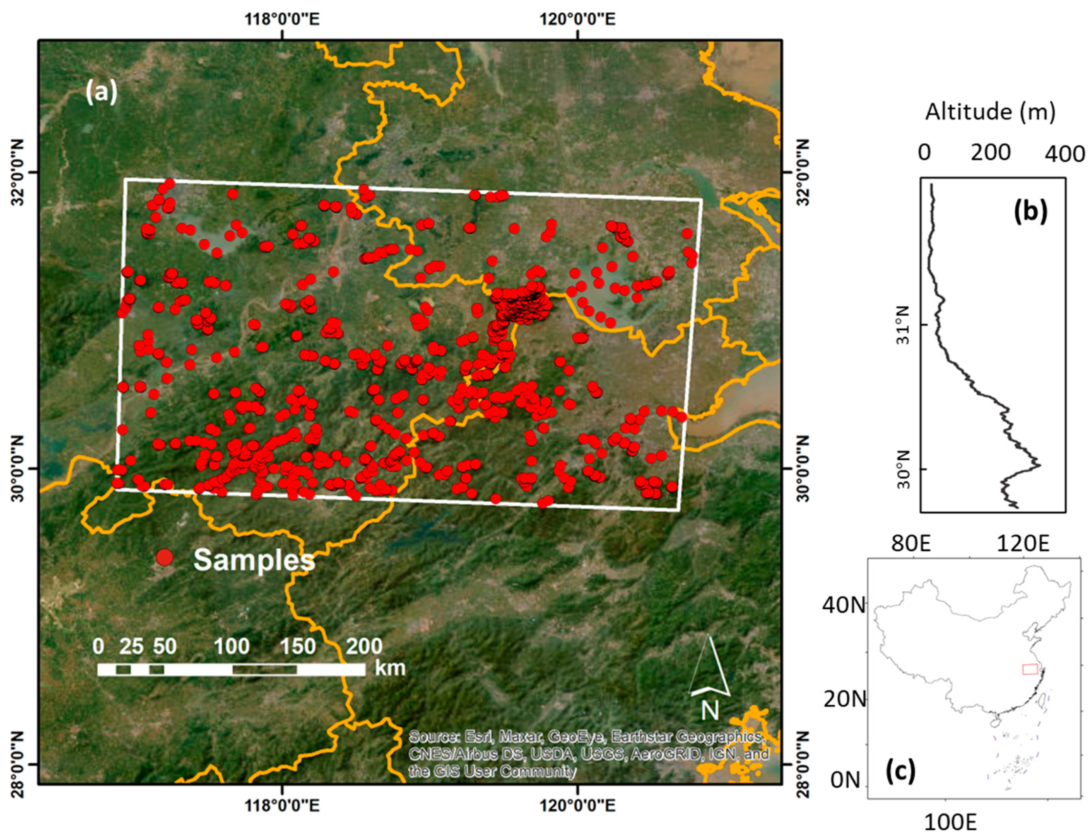
2.1. Study Area

Our focal area is in the southeastern hilly region of China, which is located at the intersection of three provinces (i.e., Anhui, Zhejiang and Jiangsu) with an area of 120,000 km2 (Figure 1). This study area has a typical subtropical monsoon climate, with a mean annual temperature of approximately 15 °C and a mean annual precipitation of approximately 1000 mm yr−1. The fertile and humid condition makes it an ideal place for bamboo growth. Therefore, there is a long history of bamboo cultivation. This area is a typical region where bamboo and woody forest both account for a considerable proportion [34]. The northern part is a plain (altitude < 50 m) with considerable areas of wheat and rice fields, as well as large areas of open water such as Taihu Lake. Woody and bamboo forests are mainly distributed in the southern hilly part (altitude > 200 m) where there are less croplands.

2.2. Data

2.2.1. Field Samples

Field samples were collected during the field survey in 2020 (Figure 1). The field trip was designed to randomly distribute and cover the entire study area. Samples that were not located in homogeneous patches (i.e., anomalous reflectance in a 3 × 3 spatial domain) were removed using manual quality control. Finally, a total of 909 samples shown in Figure 1 were used, covering seven categories: evergreen woody forest (240 samples), deciduous woody forest (119 samples), bamboo forest (238 samples), cropland (218 samples), open water surface (12 samples), artificial surface (44 samples) and barren (38 samples). Shrubland is rarely distributed in this region and is ignored in the current study. Aforementioned field campaigns were carried out focusing on vegetation categories. To avoid model bias towards the categories with larger sample sizes, we manually supplemented samples for artificial surface and an open water surface (45 and 27, respectively) based on existing land cover products and very high-resolution imagery [21,35]. Seventy percent of all field samples were randomly selected as a training set (687), with the other thirty percent as the validation set (294). It should be noted that all bamboo forests in this study are moso-bamboo, which accounts for a majority of the total bamboo forest area in China [36].

2.2.2. Remote Sensing Data

We used three different remote sensing products to map bamboo forests in this study: optical bands and derived metrics from Sentinel-2; topography information derived from the Shuttle Radar Topography Mission (SRTM) with 90-m resolution [37]; and a wall-to-wall tree height product with 30-m resolution [33]. All involved data are publicly available (Table 1).
In total, 4707 images from the Sentinel-2 level-2A surface reflectance (SR) product were collected and processed to provide time-series spectral features from 2019 and 2020. A state-of-the-art method based on machine learning provided pixelwise cloud probability [38]. We adapted a 10% threshold to mask the pixels with cloud contamination. Original Sentinel2 imagery has a temporal interval of 5-days. Time-series reflectance was composited into a monthly median. Six optical bands were selected as the input: blue, green, red, red-edge, near infrared (NIR-1), and shortwave near infrared (SWIR-2). Additionally, five vegetation indices were used; the normalized difference vegetation index (NDVI), enhanced vegetation index (EVI) [39], green chlorophyll vegetation index (GCVI) [40], MERIS terrestrial chlorophyll index (MTCI) [41] and land surface water index (LSWI) [42]. The equations of the selected vegetation indices are shown in Table 2.
Since the typical RF classification algorithm shows weak capacity in fully utilizing the temporal behavior for classes with evolution over time [29] (e.g., forest categories in this study), we generated four phenology features based on time-series patterns to highlight the difference between different forests (Figure 2). We can observe that the annual peak EVI and red-edge reflectance ( d i f f E V I in Figure 2b and d i f f r e d e d g e in Figure 2c) can describe the difference in peak canopy greenness between on- and off-year bamboo forests. It should be noted that this difference in the greenness signal can be affected by annual meteorological conditions. The bamboo forests have a denser canopy, i.e., a stronger greenness signal, in on-year [28], thus creating a different absolute d i f f E V I and d i f f r e d e d g e   compared with woody forests. However, the widely used NDVI fails to detect this feature due to its saturation in densely vegetated areas (Figure 2a). In addition, bamboo forests produce more new shoots in on-years. These shoots have a faster growth rate to maturity during the green-up season (spring and early summer, shaded period in Figure 2). The growth rate can be reflected by EVI and red-edge reflectance (dashed line in Figure 2, represented by s l o p e E V I and s l o p e r e d e d g e respectively), and is helpful to differentiate bamboo from other categories. Therefore, these four phenology features ( d i f f E V I , d i f f r e d e d g e , s l o p e E V I , and s l o p e r e d e d g e ) are calculated and composited with other features.
To represent the horizontal morphology features, we used GLCM-derived features suggested by Liu et al. (2018) [26] and Qi et al. (2022) [1]: calculate the first component image from a principal component analysis (PCA) on a yearly maximum composition of all bands [1,26]. Since Lu et al. (2014) showed that some of the GLCMs were well correlated, two related metrics, homogeneity and variance, were then calculated using a moving window [43]. It should be noted that the GLCM features were calculated based on Landsat imagery with a 9 × 9 moving window in previous studies, and we adjusted it to 18 × 18 to enable the morphological features to be detected from the same spatial domain.
A wall-to-wall tree height product, which was produced based on the neural network guided interpolation method (NNGI) for 2019, was composited with the aforementioned features [33]. This product integrates spaceborne Light Detection and Ranging (LiDAR) observations and Sentinel-2 images. Compared with regression-based tree height products, NNGI overcomes the saturation effect of optical bands benefiting from spatial interpolation. Additionally, more field-samples and air-drone LiDAR were used to constrain the network in China, leading to a more satisfying accuracy than global-scale tree height products.

2.2.3. Statistical Data
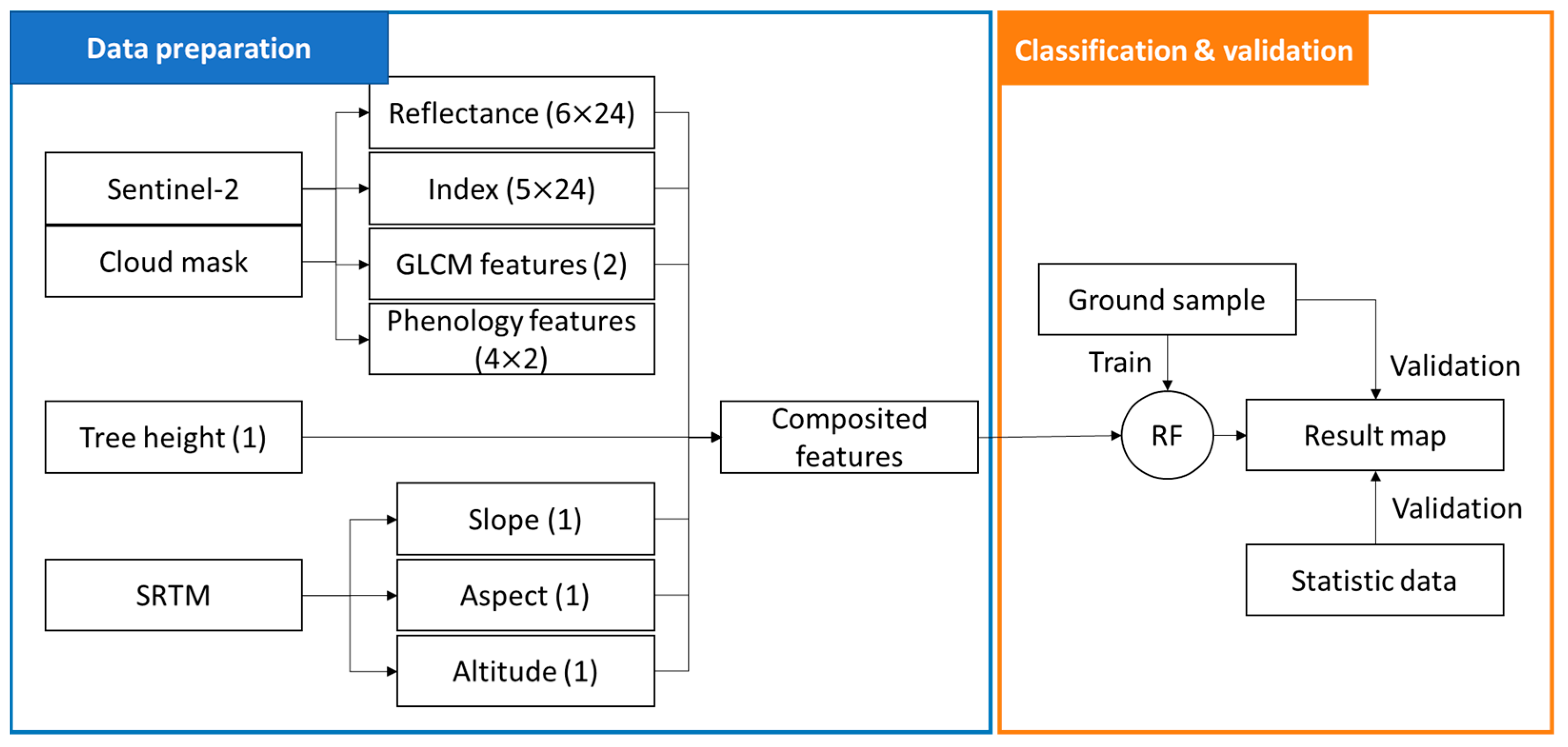
We collected country-scale bamboo forest areas in statistical reports from China’s Third National Land Survey. This nationwide survey started in 2017 and integrated commercial satellite images with extremely high spatial resolution (finer than 10 m grid), unmanned aerial vehicle images and an enormous artificial interpretation. A total of 126 counties’ entire area are covered by the current study area. Bamboo area results from 82 of them are available online and were collected.

2.3. Workflow

A typical GEE-based classification workflow was employed in this study (Figure 3). All Sentinel-2 images covering the spatial and temporal range of this study were collected using a filter. Cloud pixels on all images were masked with the corresponding cloud probability product. The monthly median reflectance for each grid was then reduced. This processed time-series reflectance was then employed to calculate indices and phenology features: the fitting slope of the red edge and EVI during the spring season and the difference in annual peak values and morphology features. Static features such as tree height and topography were also composited with time-series features. All features were then input into an RF classifier with 300 trees and a minimum of five nodes for each tree. The resulting map with 10 m spatial resolution was evaluated using the validation set of field samples and statistical data.
Overall accuracy (OA), F1-score, and the confusion matrix were selected for the accuracy assessment to evaluate model performance. OA is the most intuitive performance measure, and it is simply a ratio of correctly predicted observations to the total observations, which can be written as:
O A = S d / n × 100 ,
where S_d is the total number of correctly classified targets and n is the total number of validation targets.
The user’s accuracy (UA) measures the fraction of true positive detections ( X i j / X j × 100 ), and the producer’s accuracy (PA) measures the fraction of correctly identified positives ( X i j / X i × 100 ), where X i j is the observation in row i column j in the confusion matrix, X i is the marginal total of row i and X j is the marginal total of column j in the confusion matrix. These two metrics reflect the portion of samples that were correctly identified and the portion of samples that were correctly identified. The F1-score is the harmonic average of UA and PA:
F 1 score = U A × P A U A + P A × 2 ,
Additionally, we employed an importance score for each feature to evaluate the discriminative power of all input features, especially the contribution from newly designed features [1].

3. Results

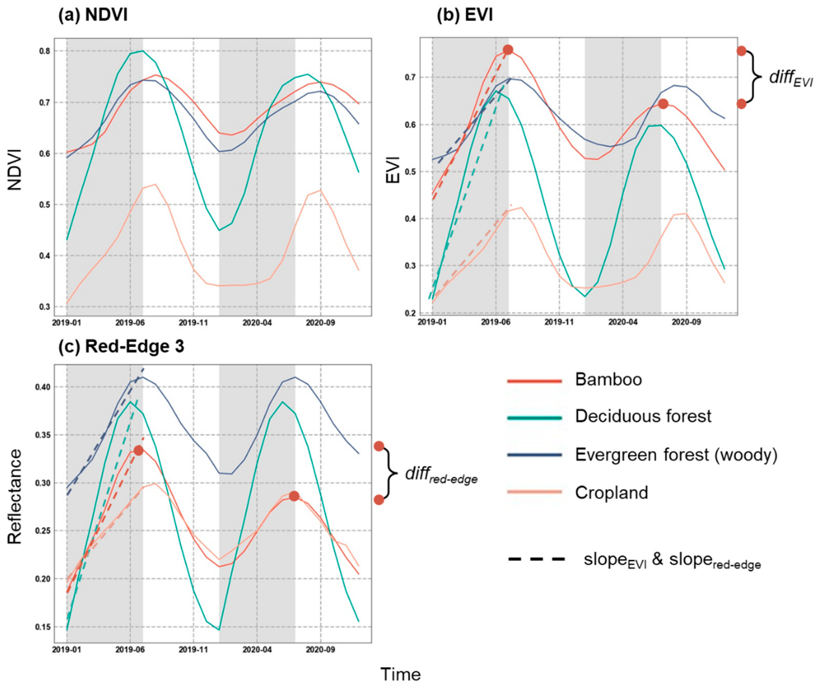
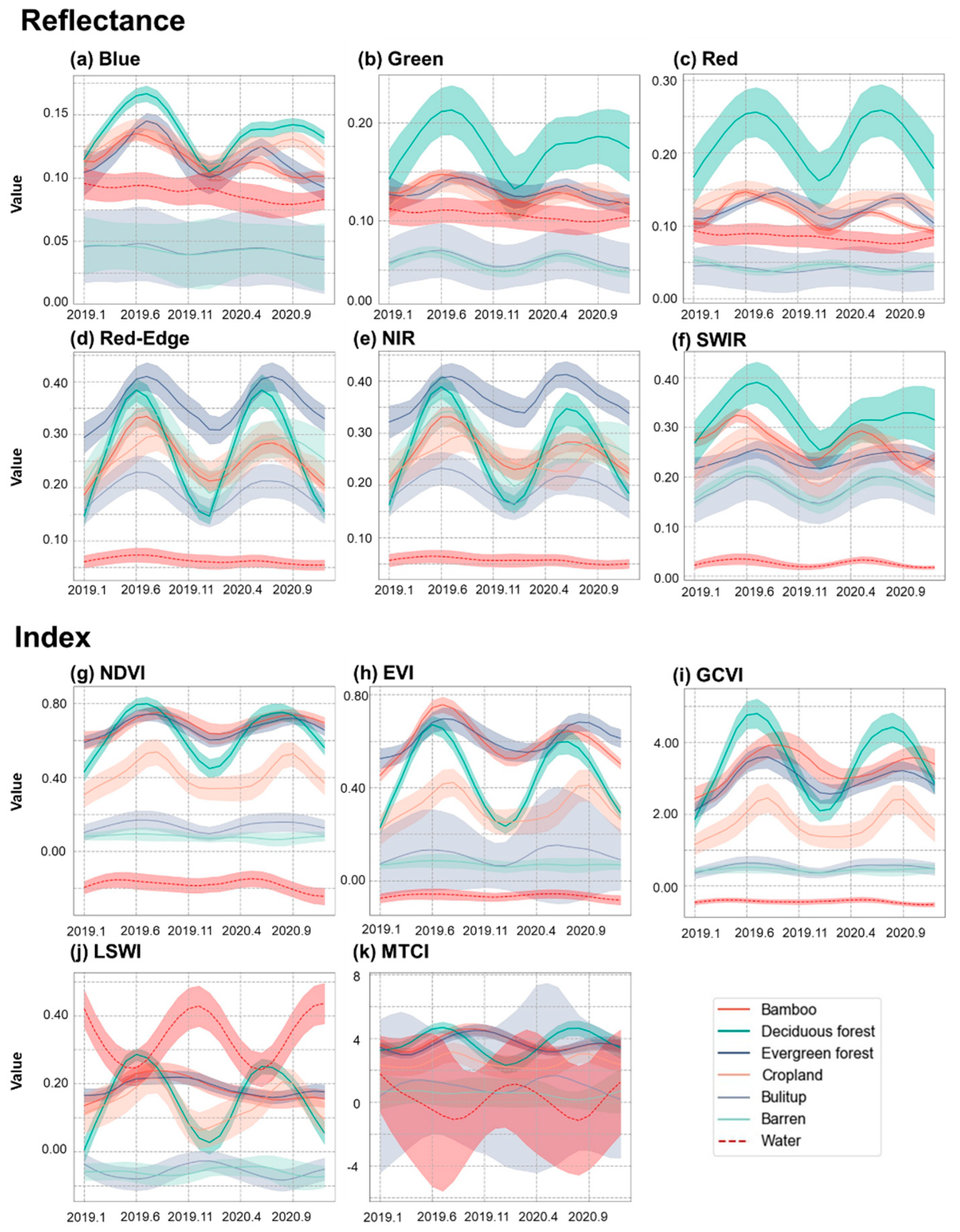
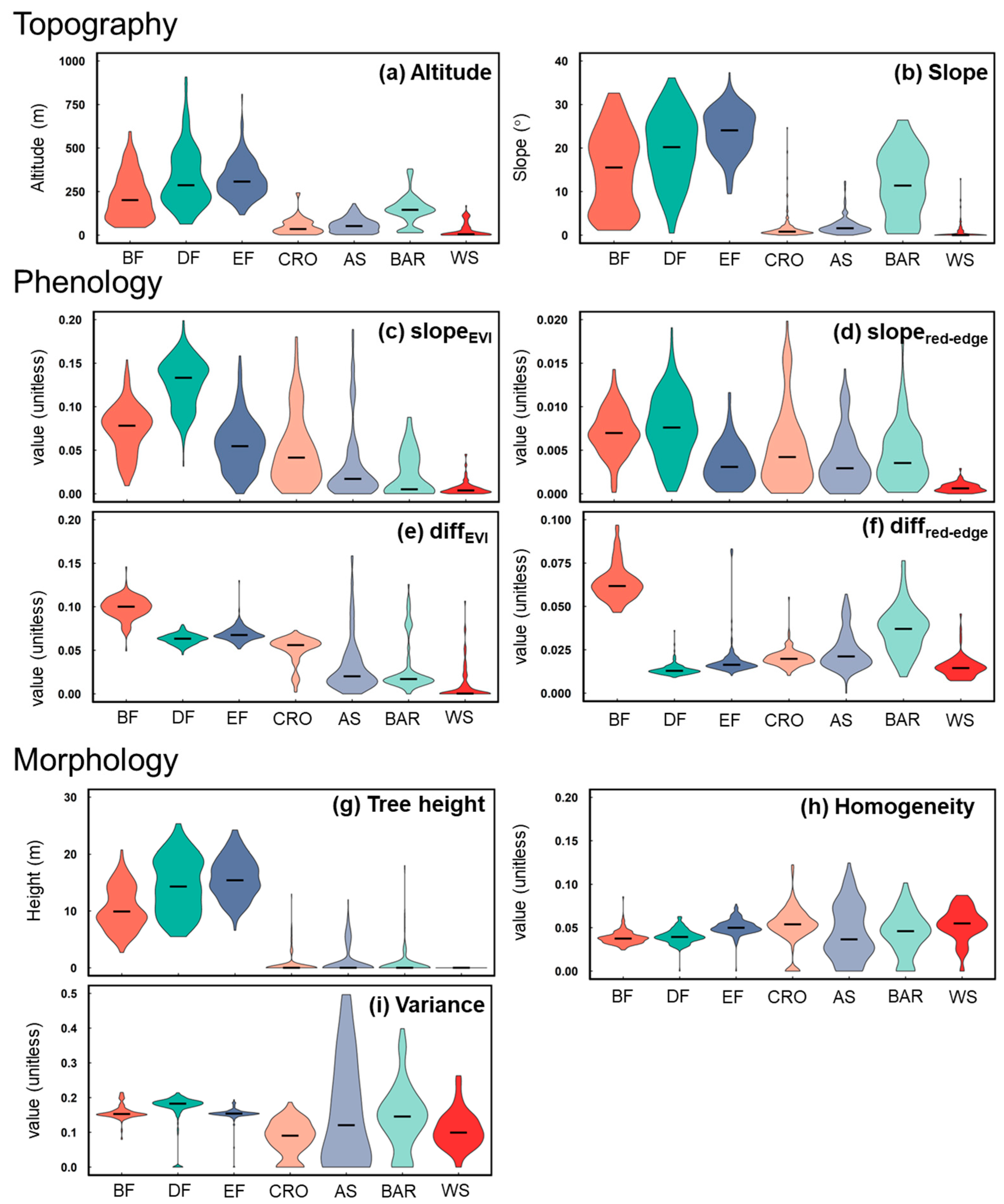
3.1. Patterns for Time-Series and Static Features

Overall, the time-series patterns of reflectance and index provide sufficient information for classification (Figure 4). All vegetation categories (bamboo forests, woody forests, and croplands) exhibit periodical reflectance patterns, i.e., annual cycles of green-up in spring and summer and senescence in autumn and winter (Figure 4a–f). A combination of information from RS bands and indices helped to differentiate these three categories. For example, evergreen woody forest has a stronger reflectance in the red-edge and NIR bands, while cropland has lower NDVI and GCVI values throughout the growing season since the herbal crop species in this region (mainly winter wheat and rice) have limited canopy height and leaf area. Although deciduous forest only occupies a limited part of the study area, its unique strong reflectance in the green and red bands during the summer season can easily be detected. However, the difference between bamboo forests and evergreen woody forests exhibited a close temporal trend and magnitude for vegetation indices, indicating that merely employing spectral band-derived indices may have failed to differentiate these two categories. Non vegetation categories (barren, artificial surface and open water surface) exhibited less temporal variance than vegetation categories.
Topography patterns also helped to constrain the classification (Figure 5a,b). The three forest categories are more likely to be distributed in hill regions with steep slopes, while cropland and artificial surfaces are mainly distributed in plain regions (altitude < 100 and slope < 5°). It should also be noted that the open water surface can hardly be distributed on the slope, which was also reported by a previous study [10].
The newly designed phenology features enhanced the bamboo mapping (Figure 5c–f). The fitting slope of the EVI in the green-up season shows that the growing efficiency of bamboo forest was weaker than that of deciduous forest but was stronger than that of other vegetation categories. The peak value difference of EVI and red edge reflectance demonstrated that the unique phenological pattern of bamboo forest can be quantified and help the classification.
Among all three morphological features, tree height makes the strongest contribution to differentiating forest (usually 10–30 m) and non forest categories (usually shorter than 5 m). However, we did not find a significant difference among categories from the two texture bands (homogeneity and variance), indicating their limited contribution to the classification results.

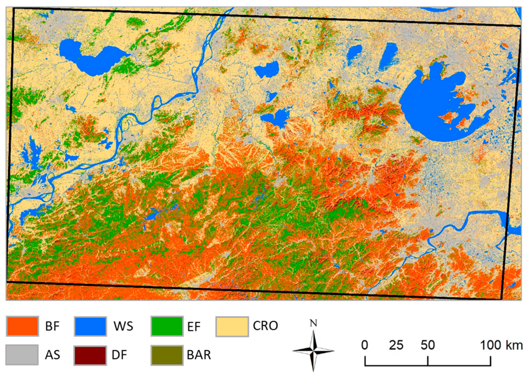
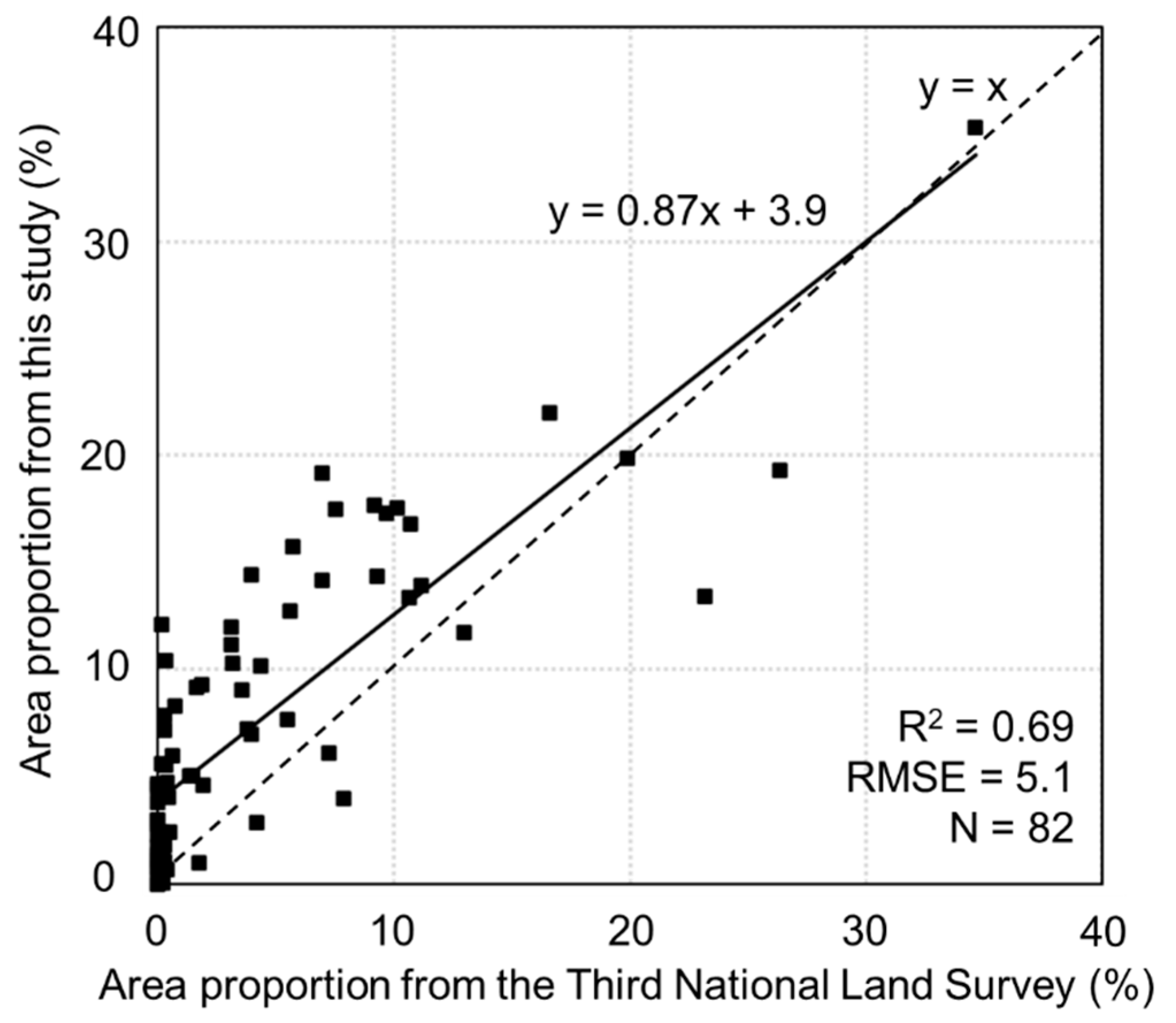
3.2. Classification Results

The classification result revealed that croplands, water surfaces and artificial surfaces are mainly distributed in the north plain whereas forest is mainly distributed in the south hill region (Figure 6). Bamboo forests are located more in the lower part of mountains with gentler slopes than woody forests, which benefits residents for management and harvesting. This pattern is also indicated in Figure 5a,b. Due to the humid and warm climate in our study area, there is only a sparse distribution of deciduous forest and barren land (<2% for both). The location and shape of the water surface and artificial surface agree with existing land cover product [21].
A comparison against field samples demonstrated the satisfactory accuracy of the classification result: OA = 89, and >80% of F1-score for vegetation categories (Table 3). Although bamboo forests and evergreen woody species exhibit similar temporal patterns in visible bands and NDVI, the F1-score of these two categories indicated a satisfactory classification performance (0.91 and 0.92, respectively). This distinction was contributed by the difference in red-edge bands (Figure 4d) and the constraints from newly designed phenology features (Figure 5e, f). The limited area proportion of deciduous forest and thus limited sample amounts led to an F1-score of 0.83. Our method can also differentiate forests and croplands with a satisfying performance (F1-score = 0.94). This success was attributed to two reasons. First, crops in this region are mainly herbivorous species such as winter wheat and summer maize, leading to lower VIs during growing season (Figure 4). Second, most of the croplands are distributed in plain regions without a slope, indicating that the terrain information helps to constrain the results (Figure 5). Given that croplands and forests both exhibit similar periodic parabolic patterns for several bands and indices, this result demonstrates that the success of tree height features can constrain the classification result. Artificial surfaces and barren land have similar patterns for most of the features and sometimes contain each other, causing a diminution in result accuracy (0.73 and 0.67, respectively).
The comparison against the National Land Survey supports the robustness and accuracy of our method (Figure 7). The bamboo area proportion in 82 counties agrees well with the result using extremely high-resolution images with intensive artificial interpretation (R2 = 0.69 and RMSE = 5.1), indicating that the automatic workflow of our method significantly reduced human labor while achieving a comparable accuracy. However, there is an overestimation of the bamboo area in the counties with approximately 10,000 ha of bamboo forests. Most of these counties have a high heterogeneity, i.e., bamboo grows in small patches surrounded by cropland or woody forest patches. The fuzzy boundary of patches leads to a mismatch of classification results based on different input resolutions and thus to this mismatch of result areas.

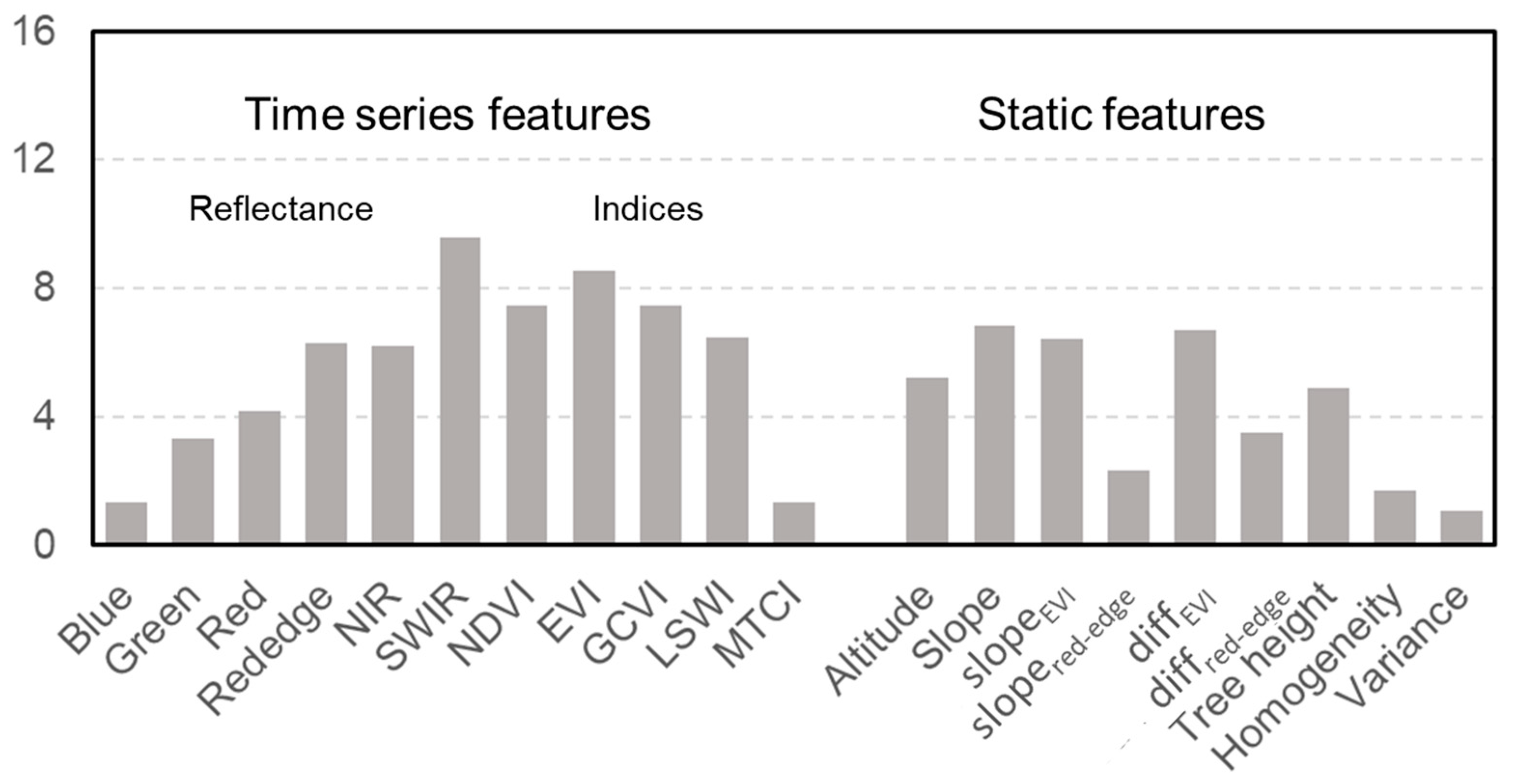
3.3. Feature Contribution

Time-series reflectance and indices contributed more to the result than static features (Figure 8). The SWIR band acted as the most important input feature (9.6%). NDVI, EVI, GCVI and LSWI are all important to the result (approximately 8%). The blue band and MTCI exhibited only approximately 1% relative importance. As static features, altitude, slope, fitting slope for EVI, interannual difference of peak value for EVI, and tree height contributed more to the result (also see Figure 5). This result also supports the reasonability of the newly designed phenology and vertical morphology features in this study. The importance of homogeneity and variance was less than 1%, indicating the limited contribution from horizontal morphology features.

4. Discussion

4.1. Success of Mapping Bamboo Forests Based on Phenology and Morphology Features

In this study, we mapped large-scale bamboo forests following the typical end-to-end classification workflow on GEE as previous studies have undertaken and incorporated the unique phenology features caused by the bamboo on- and off-year cycle and used vertical and horizontal morphology features to constrain the classification. The results in Section 3.1 have demonstrated that the aforementioned features provided sufficient information for differentiating bamboo forests from other vegetation and non vegetation categories. All features together contribute to a reasonable resulting map and a satisfactory resulting accuracy (see Section 3.2). The OA in this study was close to the accuracy of existing bamboo classifications (0.93 in [1] and 0.92 in [44]). Additionally, we received a better UA than Qi et al. (2022), indicating that our method missed less bamboo forest by including phenological features. Although there is a mismatch of spatial resolution between the bamboo map in this study (10 m) and the result of the National Land Survey (less than 10 m), and a difference between the classification systems, the comparison shows a satisfactory consistency. However, there are some counties, such as Dangtu and Tongxiang, with sparse bamboo areas reported by the National Land Survey, but greater than 5% of the bamboo area detected in this study, which reduces the R-square of Figure 7. Most of these counties are located in the northern part of the study area and have small bamboo patches. Future comparison with the bamboo map from the National Land Survey will improve our classification. An object-oriented classification may also improve our bamboo mapping by reducing the salt-pepper noise. Last but not least, the results in Section 3.3 support that the newly designed phenology and tree height features contribute substantially to the result, indicating the reasonability of our method.
The main reason for achieving the aforementioned success and the novelty of our method was because we used unique phenological features for bamboo classification. Commonly used classification algorithms, such as the random forest, have limited capacity to utilize the intrinsic logical constraint from time-series signals, i.e., the order of the signal has a rare influence on the results [29]. This means that although unique phenology patterns of bamboo forests have been reported [28], these patterns may not be detected and utilized in some applications. We bypassed this shortcoming by employing artificially designed phenological features based on time-series RS signals; fitting the slope of the green-up season and the deficit between the annual peak EVI and red-edge reflectance. The two slope-based features describe the growing efficiency during the green-up season, and the two differences in peak values describe the interannual difference in canopy density and greenness. These features were designed to show that the unique temporal signal can be detected and can magnify the difference between vegetation categories (Figure 5c–f) but do not break the end-to-end workflow, which is suitable for being transplanted. Additionally, incorporating this newly designed phenological feature scheme into an RF-based classifier not only provides an important structural tendency (represented by the increase in NDVI and EVI), but can also indicate the biochemical tendency if the calculation of increasing slope is extended to other spectral bands.
We also employed three morphology features, the LiDAR-based tree height product and two texture features, to constrain the classification. The results in Section 3 demonstrate that the tree height feature contributes to the classification. Compared with previous space-borne LiDAR sensors, the GEDI has a smaller footprint (25 m diameter) and higher sampling density, making it possible to map tree height with a 30 m resolution covering a large area. Although this information is helpful in differentiating forest and non forest categories, it has not yet been widely applied in large-scale classification. In addition to the tree height feature (usually the 95% percentile height of the canopy) [32], the GEDI also provides a vertical profile described by the full waveform signal for each footprint. Since some of the forest categories, such as bamboo and other artificial forests, have simpler vertical structures than natural forest categories under the same climate conditions, the vertical profile can be utilized to extend the field samples in the future.

4.2. Mapping Bamboo at a Larger Scale

The newly designed phenology and morphology features would also benefit bamboo mapping at a larger scale. We collected 981 samples covering the main categories in the current study with satisfactory quality, which is sufficient for training the classification. However, this density would not be maintained if we extended the spatial range in future studies since large-scale field surveys usually require unacceptable human labor and historical samples in some applications are not available. The condition would be even more difficult when the focus category is bamboo forest. Increasing the sparsity of the training set can lead to a less satisfactory result accuracy. The newly designed features can help to maintain the OA of classification when we artificially decrease the training samples (Figure 9). As can be concluded, incorporating the new feature scheme slightly improves the result accuracy under the default training strategy (1% better), but significantly increases the accuracy if the training set is reduced by 30%. We believe that this feature engineering based on plant physiology and phenology knowledge will make the classification algorithm work better in future large-scale applications which lack a sufficient sample density.
Cloud contamination is another inevitable issue for large-scale bamboo classification based on optical features. Bamboo forests in China are more likely to be distributed in humid and warm climates, indicating a considerable cloud frequency (76%, Figure 10). Bamboo forests in Southeast Asia, America and Africa also have such habitats [45]. In this study, we employed imagery from Sentinel-2 to provide time-series features. More than 85% of pixels have over 20 effective observations (24 in total for the two years). This proportion will be greatly reduced if we extend the region to the entire area of China and southeast Asia, leading to a possible loss of key phenology features such as the peak EVI [44]. Unlike the large scale classification in existing literatures [10,14], no synthetic aperture radar (SAR) images were employed in this study, although they are capable of penetrating clouds and can therefore provide observations under most weather conditions [46]. Compared with other wavelengths, C-band SAR has a medium penetration depth into the canopy to reflect structural information for the top canopy layer [47]. A state-of-the-art self-supervised SAR denoising method with a satisfactory denoising and feature restoration performance will make it a promising dataset for mapping bamboo forests [48]. However, SAR signals contain different physical information compared to spectral bands [45], and the phenological feature scheme needs to be adjusted based on the temporal tendency of SAR.

4.3. The Optimal Time Window for Bamboo Classification

In this study, we used 24 monthly composites to describe the temporal tendency of RS reflectance and indices (from January 2019 to December 2020). However, it does not indicate that the length of temporal features is necessary to achieve the classification performance in this study. To illustrate this, we conducted extra experiments using time windows with varying lengths (Table 4). All experiments used reflectance and index features, but no phenological and morphological features. For each time window, we ran classifications for all possible time windows between 2019 and 2020. For example, the experiment using a 1-month time window would have 24 classifications, referring to 24 months in 2019 and 2020. Features from a single month led to poorly performing and unstable classifiers, i.e., the average F1-score and OA were low and the standard deviation was large. A one-year length provided sufficient discrimination between different classes and reached an OA of 0.87. Using a longer window (e.g., 24-months) helped identify bamboo, as it highlighted the unique phenological patterns of on-year/off-year bamboos, whereas the improvements in other classes were limited. There is a phenomenon that the result accuracy would improve if more images from the first half of the years (i.e., the green-up season, Jan. to Jun.) were employed, which supports the reasonability of the newly designed phenological features in this study. This conclusion implies that employing an extra band selection to select the most useful bands and reduce the calculation may improve the efficiency of the large scale application [31]. Overall, we conclude that the classification performance was improved by employing features from a lengthier time window. The longer the time period is, the more distinguishable are phenological features of bamboo forests. However, considering the tradeoff between performance and efficiency, a reasonable length of time window is between 12 months or 24 months.

5. Conclusions

In this study, we have mapped large-scale bamboo forests following the typical end-to-end classification workflow on GEE, which incorporates phenology features describing the unique on- and off-year pattern for bamboo forests. We have also employed a wall-to-wall tree height product, together with two texture features, to describe the morphology features. The experiment was carried out in the southeastern hilly region of China, where bamboo forests occupy a proportionately large area. The unique pattern of bamboo forests can be detected using time-series features from optical images and static features. A satisfactory result accuracy against field samples and statistics can thus be expected and achieved. Since employing the newly designed phenology and morphology features significantly reduces the requirement of training set size, we hope to further develop this method with features from SAR images and map bamboo forests on a larger scale.

Author Contributions

Conceptualization, X.F., S.T. and Y.D.; methodology, X.F., S.T. and X.Z.; software, X.F., S.T. and X.Z.; validation, X.F. and S.T.; formal analysis, X.F., S.T. and X.Z.; investigation, X.F. and S.T.; resources, X.F., S.T. and Y.D.; data curation, X.F. and J.X.; writing—original draft preparation, X.F. and S.T.; writing—review and editing, X.F., S.T., L.Z. and L.Y.; visualization, S.T.; supervision, Y.D.; project administration, Y.D.; funding acquisition, Y.D. and S.T. All authors have read and agreed to the published version of the manuscript.

Funding

This work was sponsored by the National Natural Science Foundation of China (72140005), and in part by the National Natural Science Foundation of China (42001356), Foundation of Jiangsu Educational Committee (No. 20KJD170006), CCF-Tencent Open Fund, and CCF- AFSG Research Fund.

Data Availability Statement

The datasets generated during and/or analyzed during the current study are available from the corresponding author on reasonable request.

Acknowledgments

We acknowledge the contribution from East China Survey and Planning Institute, National Forestry and Grassland Administration and Huaiyin Institute of Technology in collecting and processing field samples.

Conflicts of Interest

The authors declare no conflict of interest.

References

  1. Qi, S.; Song, B.; Liu, C.; Gong, P.; Luo, J.; Zhang, M.; Xiong, T. Bamboo Forest Mapping in China Using the Dense Landsat 8 Image Archive and Google Earth Engine. Remote Sens. 2022, 14, 762. [Google Scholar] [CrossRef]
  2. Jian, J.; Jiang, H.; Zhou, G.; Jiang, Z.; Yu, S.; Peng, S.; Liu, S.; Wang, J. Mapping the vegetation changes in giant panda habitat using Landsat remotely sensed data. Int. J. Remote Sens. 2011, 32, 1339–1356. [Google Scholar] [CrossRef]
  3. Manandhar, R.; Kim, J.-H.; Kim, J.-T. Environmental, social and economic sustainability of bamboo and bamboo-based construction materials in buildings. J. Asian Archit. Build. Eng. 2019, 18, 49–59. [Google Scholar] [CrossRef] [Green Version]
  4. Ben-Zhi, Z.; Mao-Yi, F.; Jin-Zhong, X.; Xiao-Sheng, Y.; Zheng-Cai, L. Ecological functions of bamboo forest: Research and application. J. For. Res. 2005, 16, 143–147. [Google Scholar] [CrossRef]
  5. Zhou, G.; Meng, C.; Jiang, P.; Xu, Q. Review of carbon fixation in bamboo forests in China. Bot. Rev. 2011, 77, 262–270. [Google Scholar] [CrossRef]
  6. Liu, Z.; Deng, Z.; He, G.; Wang, H.; Zhang, X.; Lin, J.; Qi, Y.; Liang, X. Challenges and opportunities for carbon neutrality in China. Nat. Rev. Earth Environ. 2022, 3, 141–155. [Google Scholar] [CrossRef]
  7. Churkina, G.; Organschi, A.; Reyer, C.P.; Ruff, A.; Vinke, K.; Liu, Z.; Reck, B.K.; Graedel, T.; Schellnhuber, H.J. Buildings as a global carbon sink. Nat. Sustain. 2020, 3, 269–276. [Google Scholar] [CrossRef]
  8. Dong, J.; Kuang, W.; Liu, J. Continuous land cover change monitoring in the remote sensing big data era. Sci. China Earth Sci. 2017, 60, 2223–2224. [Google Scholar] [CrossRef]
  9. Sonobe, R.; Yamaya, Y.; Tani, H.; Wang, X.; Kobayashi, N.; Mochizuki, K.-I. Crop classification from Sentinel-2-derived vegetation indices using ensemble learning. J. Appl. Remote Sens. 2018, 12, 026019. [Google Scholar] [CrossRef] [Green Version]
  10. Zhang, X.; Wu, B.; Ponce-Campos, G.E.; Zhang, M.; Chang, S.; Tian, F. Mapping up-to-date paddy rice extent at 10 m resolution in china through the integration of optical and synthetic aperture radar images. Remote Sens. 2018, 10, 1200. [Google Scholar] [CrossRef]
  11. Yeom, J.; Jung, J.; Chang, A.; Ashapure, A.; Maeda, M.; Maeda, A.; Landivar, J. Comparison of vegetation indices derived from UAV data for differentiation of tillage effects in agriculture. Remote Sens. 2019, 11, 1548. [Google Scholar] [CrossRef] [Green Version]
  12. Xiao, X.; Boles, S.; Liu, J.; Zhuang, D.; Frolking, S.; Li, C.; Salas, W.; Moore III, B. Mapping paddy rice agriculture in southern China using multi-temporal MODIS images. Remote Sens. Environ. 2005, 95, 480–492. [Google Scholar] [CrossRef]
  13. Campos, J.C.; Sillero, N.; Brito, J.C. Normalized difference water indexes have dissimilar performances in detecting seasonal and permanent water in the Sahara–Sahel transition zone. J. Hydrol. 2012, 464, 438–446. [Google Scholar] [CrossRef]
  14. Tian, F.; Wu, B.; Zeng, H.; Zhang, X.; Xu, J. Efficient identification of corn cultivation area with multitemporal synthetic aperture radar and optical images in the google earth engine cloud platform. Remote Sens. 2019, 11, 629. [Google Scholar] [CrossRef] [Green Version]
  15. Belgiu, M.; Csillik, O. Sentinel-2 cropland mapping using pixel-based and object-based time-weighted dynamic time warping analysis. Remote Sens. Environ. 2018, 204, 509–523. [Google Scholar] [CrossRef]
  16. Vuolo, F.; Neuwirth, M.; Immitzer, M.; Atzberger, C.; Ng, W.-T. How much does multi-temporal Sentinel-2 data improve crop type classification? Int. J. Appl. Earth Obs. Geoinf. 2018, 72, 122–130. [Google Scholar] [CrossRef]
  17. Chen, Z.; White, L.; Banks, S.; Behnamian, A.; Montpetit, B.; Pasher, J.; Duffe, J.; Bernard, D. Characterizing marsh wetlands in the Great Lakes Basin with C-band InSAR observations. Remote Sens. Environ. 2020, 242, 111750. [Google Scholar] [CrossRef]
  18. Hill, R.; Wilson, A.; George, M.; Hinsley, S. Mapping tree species in temperate deciduous woodland using time-series multi-spectral data. Appl. Veg. Sci. 2010, 13, 86–99. [Google Scholar] [CrossRef]
  19. Gilmore, M.S.; Wilson, E.H.; Barrett, N.; Civco, D.L.; Prisloe, S.; Hurd, J.D.; Chadwick, C. Integrating multi-temporal spectral and structural information to map wetland vegetation in a lower Connecticut River tidal marsh. Remote Sens. Environ. 2008, 112, 4048–4060. [Google Scholar] [CrossRef]
  20. Madonsela, S.; Cho, M.A.; Mathieu, R.; Mutanga, O.; Ramoelo, A.; Kaszta, Ż.; Van De Kerchove, R.; Wolff, E. Multi-phenology WorldView-2 imagery improves remote sensing of savannah tree species. Int. J. Appl. Earth Obs. Geoinf. 2017, 58, 65–73. [Google Scholar] [CrossRef]
  21. Liu, H.; Gong, P.; Wang, J.; Clinton, N.; Bai, Y.; Liang, S. Annual dynamics of global land cover and its long-term changes from 1982 to 2015. Earth Syst. Sci. Data 2020, 12, 1217–1243. [Google Scholar] [CrossRef]
  22. Petitjean, F.; Inglada, J.; Gançarski, P. Satellite image time series analysis under time warping. IEEE Trans. Geosci. Remote Sens. 2012, 50, 3081–3095. [Google Scholar] [CrossRef]
  23. Hansen, M.C.; Potapov, P.V.; Moore, R.; Hancher, M.; Turubanova, S.A.; Tyukavina, A.; Thau, D.; Stehman, S.V.; Goetz, S.J.; Loveland, T.R. High-resolution global maps of 21st-century forest cover change. Science 2013, 342, 850–853. [Google Scholar] [CrossRef] [PubMed] [Green Version]
  24. Sun, X.; Han, N.; Ge, H.; Gu, C. Multi-scale segmentation, object-based extraction of moso bamboo forest from SPOT5 imagery. Sci. Silvae Sin. 2013, 49, 80–87. [Google Scholar]
  25. Gorelick, N.; Hancher, M.; Dixon, M.; Ilyushchenko, S.; Thau, D.; Moore, R. Google Earth Engine: Planetary-scale geospatial analysis for everyone. Remote Sens. Environ. 2017, 202, 18–27. [Google Scholar] [CrossRef]
  26. Liu, C.; Xiong, T.; Gong, P.; Qi, S. Improving large-scale moso bamboo mapping based on dense Landsat time series and auxiliary data: A case study in Fujian Province, China. Remote Sens. Lett. 2018, 9, 1–10. [Google Scholar] [CrossRef]
  27. Rußwurm, M.; Wang, S.; Korner, M.; Lobell, D. Meta-learning for few-shot land cover classification. In Proceedings of the IEEE/CVF Conference on Computer Vision and Pattern Recognition Workshops, Virtual, 14–19 June 2020; pp. 200–201. [Google Scholar]
  28. Li, L.; Li, N.; Lu, D.; Chen, Y. Mapping Moso bamboo forest and its on-year and off-year distribution in a subtropical region using time-series Sentinel-2 and Landsat 8 data. Remote Sens. Environ. 2019, 231, 111265. [Google Scholar] [CrossRef]
  29. Pelletier, C.; Webb, G.I.; Petitjean, F. Temporal convolutional neural network for the classification of satellite image time series. Remote Sens. 2019, 11, 523. [Google Scholar] [CrossRef] [Green Version]
  30. Michałowska, M.; Rapiński, J. A review of tree species classification based on airborne LiDAR data and applied classifiers. Remote Sens. 2021, 13, 353. [Google Scholar] [CrossRef]
  31. Naidoo, L.; Cho, M.A.; Mathieu, R.; Asner, G. Classification of savanna tree species, in the Greater Kruger National Park region, by integrating hyperspectral and LiDAR data in a Random Forest data mining environment. ISPRS J. Photogramm. Remote Sens. 2012, 69, 167–179. [Google Scholar] [CrossRef]
  32. Potapov, P.; Li, X.; Hernandez-Serna, A.; Tyukavina, A.; Hansen, M.C.; Kommareddy, A.; Pickens, A.; Turubanova, S.; Tang, H.; Silva, C.E. Mapping global forest canopy height through integration of GEDI and Landsat data. Remote Sens. Environ. 2021, 253, 112165. [Google Scholar] [CrossRef]
  33. Liu, X.; Su, Y.; Hu, T.; Yang, Q.; Liu, B.; Deng, Y.; Tang, H.; Tang, Z.; Fang, J.; Guo, Q. Neural network guided interpolation for mapping canopy height of China’s forests by integrating GEDI and ICESat-2 data. Remote Sens. Environ. 2022, 269, 112844. [Google Scholar] [CrossRef]
  34. Li, M.; Li, C.; Jiang, H.; Fang, C.; Yang, J.; Zhu, Z.; Shi, L.; Liu, S.; Gong, P. Tracking bamboo dynamics in Zhejiang, China, using time-series of Landsat data from 1990 to 2014. Int. J. Remote Sens. 2016, 37, 1714–1729. [Google Scholar] [CrossRef]
  35. Gong, P.; Li, X.; Wang, J.; Bai, Y.; Chen, B.; Hu, T.; Liu, X.; Xu, B.; Yang, J.; Zhang, W. Annual maps of global artificial impervious area (GAIA) between 1985 and 2018. Remote Sens. Environ. 2020, 236, 111510. [Google Scholar] [CrossRef]
  36. Li, P.; Zhou, G.; Du, H.; Lu, D.; Mo, L.; Xu, X.; Shi, Y.; Zhou, Y. Current and potential carbon stocks in Moso bamboo forests in China. J. Environ. Manag. 2015, 156, 89–96. [Google Scholar] [CrossRef]
  37. Jarvis, A.; Reuter, H.I.; Nelson, A.; Guevara, E. Hole-Filled SRTM for the Globe Version 4. CGIAR-CSI SRTM 90m Database. Available online: http://srtm.csi.cgiar.org (accessed on 12 January 2023).
  38. Skakun, S.; Wevers, J.; Brockmann, C.; Doxani, G.; Aleksandrov, M.; Batič, M.; Frantz, D.; Gascon, F.; Gómez-Chova, L.; Hagolle, O. Cloud Mask Intercomparison eXercise (CMIX): An evaluation of cloud masking algorithms for Landsat 8 and Sentinel-2. Remote Sens. Environ. 2022, 274, 112990. [Google Scholar] [CrossRef]
  39. Huete, A.; Didan, K.; Miura, T.; Rodriguez, E.P.; Gao, X.; Ferreira, L.G. Overview of the radiometric and biophysical performance of the MODIS vegetation indices. Remote Sens. Environ. 2002, 83, 195–213. [Google Scholar] [CrossRef]
  40. Gitelson, A.A.; Viña, A.; Arkebauer, T.J.; Rundquist, D.C.; Keydan, G.; Leavitt, B. Remote estimation of leaf area index and green leaf biomass in maize canopies. Geophys. Res. Lett. 2003, 30. [Google Scholar] [CrossRef] [Green Version]
  41. Dash, J.; Curran, P. The MERIS terrestrial chlorophyll index. Int. J. Remote Sens. 2004, 25, 5403–5413. [Google Scholar] [CrossRef]
  42. Wang, J.; Xiao, X.; Qin, Y.; Dong, J.; Geissler, G.; Zhang, G.; Cejda, N.; Alikhani, B.; Doughty, R.B. Mapping the dynamics of eastern redcedar encroachment into grasslands during 1984–2010 through PALSAR and time series Landsat images. Remote Sens. Environ. 2017, 190, 233–246. [Google Scholar] [CrossRef] [Green Version]
  43. Lu, D.; Li, G.; Moran, E.; Dutra, L.; Batistella, M. The roles of textural images in improving land-cover classification in the Brazilian Amazon. Int. J. Remote Sens. 2014, 35, 8188–8207. [Google Scholar] [CrossRef]
  44. Zhang, M.; Gong, P.; Qi, S.; Liu, C.; Xiong, T. Mapping bamboo with regional phenological characteristics derived from dense Landsat time series using Google Earth Engine. Int. J. Remote Sens. 2019, 40, 9541–9555. [Google Scholar] [CrossRef]
  45. Zhang, M.; Keenan, T.F.; Luo, X.; Serra-Diaz, J.M.; Li, W.; King, T.; Cheng, Q.; Li, Z.; Andriamiarisoa, R.L.; Raherivelo, T.N.A.N. Elevated CO2 moderates the impact of climate change on future bamboo distribution in Madagascar. Sci. Total Environ. 2022, 810, 152235. [Google Scholar] [CrossRef] [PubMed]
  46. Kovacs, J.M.; Jiao, X.; Flores-de-Santiago, F.; Zhang, C.; Flores-Verdugo, F. Assessing relationships between Radarsat-2 C-band and structural parameters of a degraded mangrove forest. Int. J. Remote Sens. 2013, 34, 7002–7019. [Google Scholar] [CrossRef]
  47. Touzi, R.; Deschamps, A.; Rother, G. Phase of target scattering for wetland characterization using polarimetric C-band SAR. IEEE Trans. Geosci. Remote Sens. 2009, 47, 3241–3261. [Google Scholar] [CrossRef]
  48. Tan, S.; Zhang, X.; Wang, H.; Yu, L.; Du, Y.; Yin, J.; Wu, B. A CNN-Based Self-Supervised Synthetic Aperture Radar Image Denoising Approach. IEEE Trans. Geosci. Remote Sens. 2021, 60, 1–15. [Google Scholar] [CrossRef]
Figure 1. Study area. Boundaries and field-ground truth samples are labelled in the figure (a). The altitude profile is displayed in the subpanel. The altitude profile representing the average altitude of pixels with the same latitude is displayed in the panel (b). The relative position of the study area is shown in panel (c).
Remotesensing 15 00515 g001
Figure 2. Example of time-series patterns for typical vegetation categories (bamboo, deciduous forest, evergreen woody forest and crop land). Solid lines in this figure represent the average of all field samples. The NDVI, EVI and red-edge reflectance from 2019 to 2020 are shown in panels (ac), respectively. The difference in the peak value for the EVI and red-edge band ( d i f f E V I and d i f f r e d e d g e ) is demonstrated in panels (b,c). The fitting slope for the red-edge reflectance in the green-up season (shade area) is demonstrated in panel (c).
Remotesensing 15 00515 g002
Figure 3. Workflow of this study. Data and features are represented by blocks. RF in the circle represents the random forest classifier. The numbers in the brackets represent the numbers of features and timesteps. Blue and orange colour represents the data preparation and classification-validation steps, respectively.
Remotesensing 15 00515 g003
Figure 4. Temporal patterns for different categories. (af) display the temporal patterns for the reflectance of six bands. (gk) display the temporal patterns for five vegetation indices. The shade of each line represents the standard error calculated from all field samples.
Remotesensing 15 00515 g004
Figure 5. Static patterns for different categories. The width of each violin represents the relative density at different values. The black line is the median of each category;(a,b) display the topography patterns; (cf) display the phenology patterns; (gi) display morphological patterns. BF = bamboo forest, DF = deciduous forest, EF = evergreen woody forest, CRO = cropland, AS = artificial surface, BAR = barren, WS = water surface. Different colour represents different categories.
Remotesensing 15 00515 g005
Figure 6. Spatial distribution of classification result. Abbreviation has the same meaning as in Figure 5.
Remotesensing 15 00515 g006
Figure 7. Comparison of bamboo area proportion (%) in this study and China’s Third National Land Survey. The linear fitted line and 1:1 line (y = x) are labelled in the figure by solid line and dashed line respectively. R2 represents the correlation coefficient, and RMSE represents the root mean square error. N is the number of sample plots.
Remotesensing 15 00515 g007
Figure 8. Relative importance for input features.
Remotesensing 15 00515 g008
Figure 9. Relationship between result overall accuracy and sample size (%). Two feature schemes are compared: with four phenology and three morphology features and without these seven features.
Remotesensing 15 00515 g009
Figure 10. Map of yearly global cloud frequency and terrestrial bamboo forest in mainland China. Cloud frequency is calculated using the quality control band from MODerate-resolution Imaging Spectroradiometer (MODIS) observations from 2003 to 2020. Provinces with bamboo distribution in China are labelled according to Qi et al. (2022) [1]. The boxplot in the subpanel displays the distribution of cloud frequency in this region.
Remotesensing 15 00515 g010
Table 1. Remote sensing product used in this study.
ProductVariableTime IntervalWebsite
Sentinel-2 Level 2ARS reflectanceMonthlyhttps://earth.esa.int/web/sentinel/user-guides/sentinel-2-msi/product-types/level-2a (accessed on 12 January 2023)
Vegetation indicesMonthly
PhenologyYearly
MorphologyStatic
SRTMElevationStatichttps://srtm.csi.cgiar.org/ (accessed on 12 January 2023)
Slope
Aspect
NNGITree heightStatichttp://www.3decology.org/dataset-software/ (accessed on 12 January 2023)
Table 2. Equations of selected vegetation indices. Rx represents the reflectance of band x of Sentinel-2.
IndexEquation
NDVI ( R N I R R r e d ) / ( R N I R + R r e d )
EVI 2.5 × ( R N I R R r e d ) / ( R N I R + 6 × R r e d 7.5 × R b l u e + 1 )
GCVI R N I R / R g r e e n 1
MTCI ( R N I R 2 R N I R 1 ) / ( R N I R 1 R r e d )
LSWI ( R N I R R S W I R 1 ) / ( R N I R + R S W I R 1 )
Table 3. Confusion matrix of the resulting bamboo map. Abbreviation has the same meaning as in Figure 5.
Predicted Label
BFDFEFCROASBARWSUA
Field
samples
BF654200000.92
DF432100000.86
EF336600000.92
CRO010632000.95
AS002420200.71
BAR00005700.58
WS000100100.91
PA0.900.800.930.930.740.781.00OA = 0.89
F1-score0.910.830.920.940.730.670.95
Table 4. Statistics of classification performance using different lengths of time windows. Mean value represents average resulting F1-score/OA of using all possible input feature schemes. Std is the standard error of using all possible schemes. The best performance of each category is labeled in bold.
WindowItemBFDFEFCROASBARWTOA
1-monthMean0.530.540.670.510.570.530.840.57
Std0.150.120.160.20.130.160.710.13
4-monthMean0.770.770.810.80.770.720.910.77
Std0.090.150.040.070.050.070.010.03
6-monthMean0.810.860.880.810.80.730.850.86
Std0.040.070.020.030.030.090.020.02
12-monthMean0.860.910.920.880.810.720.900.87
Std0.0200.010.010.020.070.020.03
24-monthMean0.910.90.920.900.730.670.920.88
Std--------
Disclaimer/Publisher’s Note: The statements, opinions and data contained in all publications are solely those of the individual author(s) and contributor(s) and not of MDPI and/or the editor(s). MDPI and/or the editor(s) disclaim responsibility for any injury to people or property resulting from any ideas, methods, instructions or products referred to in the content.

