A Robust Adaptive Filtering Algorithm for GNSS Single-Frequency RTK of Smartphone

Abstract

In this paper, a single-frequency real-time kinematic positioning (RTK) robust adaptive Kalman filtering algorithm is proposed in order to realize real-time dynamic high-precision positioning of smartphone global navigation satellite systems (GNSSs). A robust model is established by using the quartile method to dynamically determine the threshold value and eliminate the gross error of observation. The Institute of Geodesy and Geophysics Ⅲ (IGG Ⅲ) weight function is used to construct the position and speed classification adaptive factors to weaken the impact of state mutation errors. Based on the analysis of the measured data of Xiaomi 8 and Huawei P40 smartphones, simulated dynamic tests show that the overall accuracy of the Xiaomi 8 is improved by more than 85% with the proposed robust RTK algorithm, and the overall positioning error is less than 0.5 m in both open and sheltered environments. The overall accuracy of the Huawei P40 is improved by more than 25%. Furthermore, the overall positioning accuracy is better than 0.3 m in open environments, and about 0.8 m in blocked situations. Dynamic experiments show that the use of the robust adaptive RTK algorithm improves the full-time solution planar positioning accuracy of the Xiaomi 8 by more than 15%. In addition, the planar positioning accuracy under open and occluded conditions is 0.8 m and 1.5 m, respectively, and the overall positioning accuracy of key nodes whose movement state exhibits major changes improves by more than 20%.

1. Introduction

In recent years, microelectronics and communication technologies have developed rapidly. The current low-cost global navigation satellite system (GNSS) chipsets have become more mature in terms of signal acquisition, the anti-multipath, and the integrated navigation of multiple systems. These chipsets have been used in a large number of emerging industries such as autonomous driving, smartphone navigation, and UAV logistics. Smartphone GNSS devices account for more than 80% of the total global GNSS devices and have a large user group and diversified needs. Therefore, research on the smartphone GNSS positioning algorithm has great scientific and commercial value [1,2]. At the Google I/O conference in May 2016, Google announced that it would open the application programming interface (API) of original GNSS observations in the Android operating system, that is, the users could directly obtain the pseudo-range, carrier, Doppler, signal-to-noise ratio, and other original observation information received by smartphones through fixed APIs from Android 7. This provides the possibility of developing a GNSS positioning algorithm suitable for the characteristics of smartphone observations and improving their positioning accuracy [3,4,5,6]. Therefore, many researchers have worked on the GNSS localization algorithms of Android smartphones and have produced a significant amount of research results.

Wanninger et al. observed and analyzed the signal-to-noise ratio (SNR) of an Huawei P30 smartphone over a long time and found that the smartphone antenna was not sensitive to the L5/E5a frequency, and the SNR decreased after a long observation time [7]. Baku et al. also used an Huawei P30 to compare and analyze the influence of L1 and L5 frequencies on the positioning accuracy of the pseudo-range differential global position system (DGPS). The authors showed that a positioning accuracy of 0.4 m could be achieved by using the L5 frequency [8]. Gao et al. proposed a single-difference method between satellites to eliminate the influence of the unfixed difference between the smartphone pseudo-range and carrier phase observations. The experimental results showed that the smartphone single-frequency PPP plane positioning accuracy was 1.51 m, and the elevation positioning accuracy was 2.79 m. The plane positioning accuracy of smartphone single-frequency RTK was 0.73 m, and the elevation positioning accuracy was 0.78 m [9]. Li et al. proposed a real-time precise point positioning (PPP) method based on the smartphone data processing strategy. The authors placed the smartphones on a roof and in a vehicle for dynamic experiments. The positioning accuracy of the roof test plane was about 1 m, the elevation positioning accuracy was about 1.5 m, the positioning accuracy of the interior test plane was 1.0–1.5 m, and the elevation positioning accuracy was 1–2 m [10,11,12].

Compared with the receiver equipment, smartphones are structurally and spatially compact, and usually use the built-in linear polarization passive antenna to receive the GNSS signals. The linear polarization antenna is sensitive to satellite signals but has poor anti-multipath performance. Furthermore, the pseudo-range and carrier phase observations can contain many errors. In view of the limitations of the smartphone antenna, Geng et al. found that the smartphone GNSS chipsets had different initial phase biases (IPBs) for different satellites, which could lead to unfixed ambiguities. The u-blox ANN-MS patch antenna was used to connect to a Xiaomi 8, achieving centimeter-level static positioning accuracy [13,14]. Pesyna et al. showed that the smartphone antenna was the key to quickly and reliably solving the ambiguity fixing problem and achieving high-precision positioning accuracy [15]. Daruga et al. successfully achieved fixed ambiguity in an open environment by estimating the offset and change in the antenna phase center of an Huawei Mate20X [16].

Geng and Laurichesse et al. smoothed the pseudo-range observation values of smartphones by using Doppler and carrier phase observation values in order to reduce the gross error and improve the accuracy. The experimental results showed that the smoothed pseudo-range could significantly improve the positioning accuracy [17,18]. Wang et al. proposed a filtering algorithm for object position constrained by the phase epoch difference, which effectively smoothed the pseudo-range noise of a Xiaomi 8. In pedestrian and vehicle experiments, planar accuracies of 0.65 m and 1.03 m were achieved, respectively [19]. Guo et al. analyzed the quality of the observed values of Huawei Mate 20/30 and Xiaomi 8 smartphones, and proposed a method to eliminate the pseudo-range gross error using information such as the SNR, height angle, and pre-test and post-test residuals. The experimental results showed that the static plane accuracy and elevation positioning accuracy were better than 1 m and 2 m, respectively [20].

Some researchers also used the robust estimation method to deal with gross errors that could not be eliminated in preprocessing. Chen et al. added robust modules in the filtering process to reduce the impact of gross errors that could not be eliminated by pre-processing the positioning results. The convergence time and positioning accuracy were significantly improved for a Xiaomi 8 [21]. Zhu et al. established a GNSS mathematical model that is more suitable for smartphones and used robust Kalman filtering to make parameter notes. The experimental results showed that compared with the traditional model, the GPS/BDS/GLO horizontal and vertical RMS decreased by 23.91% and 62.06% respectively [22]. Zhang et al. proposed a random model that combined elevation and SNR. The template function of the SNR was used to estimate the unmodeled error. After using this model, the overall accuracy of RTDs in complex environments improved by more than 10% [23]. Gong et al. proposed a RWTLS-LM-IGG algorithm by combining the weighted total least squares (WTLS), Lagrange multipliers (LM), and IGG weight functions. Experiments with simulated and actual data showed that the new method can effectively weaken the influence of gross errors [24].

Kalman filtering is not robust against observation and dynamic model anomalies; therefore, it cannot obtain reliable dynamic positioning results. The observation anomaly can be estimated by a robust model, and the dynamic model anomaly is usually corrected by adaptive estimation. Peng et al. combined innovation vector robust Kalman filtering and Sage–Husa adaptive filtering. The experimental results showed that the accuracy of this method in the plane and elevation directions improved by 1 cm and 4 cm, respectively [25,26]. Su et al. proposed a mixed weighting function considering the signal-to-noise ratio and altitude angle. The experimental results showed that the hybrid weighting function can weaken the influence of the multipath on carrier phase observations and improve the RTK positioning accuracy [27]. Odijk et al. presented a closed-form expression, which enables the single-frequency PPP-RTK user to compute the variance matrix of the network corrections by themselves, and the experimental results showed that the single-frequency PPP can fix the ambiguity in 10 min, even with a low-cost receiver. The plane positioning accuracy was sub-centimeter-level and the elevation positioning accuracy was centimeter-level [28]. In summary, there is limited research on robust and adaptive algorithms for Android smartphones. The real-time kinematic positioning (RTK) is a relatively mature and widely used positioning technology that can achieve centimeter-level accuracy and meet the people’s needs of daily navigation and positioning. Therefore, this paper studies the robust adaptive algorithm for GNSS single-frequency RTK of Android smartphones.

In the following, first, we list several smartphones that support the GNSS raw data output and summarize the characteristics of smartphone observations. Secondly, the double-difference location algorithm and standard Kalman filter parameter estimation method are discussed. A new RTK location model based on the quartile robust adaptive Kalman filter is proposed, including the quartile robust model and classification adaptive factor model. Subsequently, we collect three groups of static data and dynamic data to verify the effectiveness of the quartile robust model and the classification adaptive factor model.

2. Characteristics of Smartphone Observations

Table 1. Different smartphone-receiving satellite systems and frequency bands.

Mobile Phone Type	GNSS Chipsets Type	GPS	GLONASS	GALILEO	BDS	QZSS
Xiaomi 8	Broadcom BCM47755	L1/L5	R1	E1/E5a	B1I	J1/J5
Huawei Mate 20	Hisilicon Hi1103	L1/L5	R1	E1/E5a	B1I/	J1/J5
Huawei P30	Hisilicon Hi1103	L1/L5	R1	E1/E5a	B1I/	J1/J5
Huawei P40	Hisilicon Hi1105	L1/L5	R1	E1/E5a	B1I/B1C/B2a	J1/J5

lists the receiving satellite systems and frequencies of several Android smartphones that support the GNSS raw data output in the market. Two representative smartphones, a Xiaomi 8 and Huawei P40, are used for the experiment. The Xiaomi 8 captures a small number of satellite signals, but its tracking status is relatively stable [20]. The Huawei P40 captures a large number of satellite signals, but its tracking ability is weak, and it is easy to lose its lock in complex environments [1]. As the number of L5 and E5a satellite signals received by the Xiaomi 8 and Huawei P40 is small and the overall quality is poor, the carrier phase observation value of Huawei P40 frequencies B1C and B2a cannot be analyzed. Therefore, the experimental part only calculates the single-frequency data of four systems, i.e., GPS (L1) + GLO (R1) + GAL (E1) + BDS-3 (B1I).

The GPSTest software is used to acquire the original observation data in RAW format from the smartphone. A Python program developed by us is used to convert the pseudo-range, carrier, Doppler, and SNR observation values. The analysis of the measured data reveals that under the condition of a short baseline, the positioning accuracy of the receiver GNSS RTK is centimeter-level, and that of the smartphone is decimeter- or meter-level. This is because the smartphones use consumer-grade positioning chipsets and linearly polarized antennas. At the same time, due to the high sensitivity of the linearly polarized antenna, the observation value is seriously affected by the multipath effect, which can be about 1.5–3 m.

The pseudo-range observations contain many gross errors. The pseudo-range noise is between 5 and 10 m, which is about 10 times more than the receiver noise. The cycle slip ratio of the carrier phase observation value is between 10 and 30, and the cycle slip epoch number accounts for 5–10% of the total epoch number, which exceeds 20% under severe occlusion. The SNR of the smartphone is 5–10 Db-Hz lower than that of the receiver and is between 25 and 40 dB-Hz. Most smartphones have a duty cycle mechanism in order to reduce their power consumption, which will also cause a discontinuity in the carrier phase.

3. Methods

3.1. GNSS RTK Positioning Algorithm

The inter-satellite double-difference observation model can eliminate the satellite and receiver clock errors and weaken other types of error. For a smartphone rover station j, considering B1I and L1 frequency bands of BDS and GPS, respectively, as examples, the pseudo-range and carrier-phase double-difference observation equations are established as follows [29]:

$$\left.\begin{array}{c}\nabla ∆{\tilde{\phi }}_{ij}^{pq,B}=\frac{f}{c}\nabla ∆{\rho }_{ij}^{pq,B}-\nabla ∆N_{ij}^{pq,B}-\frac{f}{c}{I}_{ij}^{pq,B}-\frac{f}{c}{T}_{ij}^{pq,B}+{\epsilon }_{\phi }^B\\ \nabla ∆{\tilde{\phi }}_{ij}^{pq,G}=\frac{f}{c}\nabla ∆{\rho }_{ij}^{pq,G}-\nabla ∆N_{ij}^{pq,G}-\frac{f}{c}{I}_{ij}^{pq,G}-\frac{f}{c}{T}_{ij}^{pq,G}+{\epsilon }_{\phi }^G\\ \nabla ∆{\tilde{P}}_{ij}^{pq,B}=\nabla ∆{\rho }_{ij}^{pq,B}-I_{ij}^{pq,B}-T_{ij}^{pq,B}+{\epsilon }_P^B\\ \nabla ∆{\tilde{P}}_{ij}^{pq,G}=\nabla ∆{\rho }_{ij}^{pq,G}-I_{ij}^{pq,G}-T_{ij}^{pq,G}+{\epsilon }_P^G\end{array}\right\}$$

(1)

where $i$ and $j$ are the reference station and smartphone rover station, respectively, $p$ and $q$ are synchronously observed reference satellites and non-reference satellites, respectively, $B$ and $G$ represent the BDS and GPS systems, respectively, $\nabla ∆$ is a double-difference operator, and $N$ represents the integer ambiguity parameter. The carrier phase observation value is denoted by $\phi$, $P$ is the pseudo-range observation value, $\rho$ is the geometric distance between stations and satellites, $c$ is the speed of light, $f$ is the frequency point, $I$ is the ionospheric delay correction, $T$ is the tropospheric delay correction, and $\epsilon$ denotes the measurement noise and multipath effects.

The double-difference model can significantly reduce the impact of ionospheric and tropospheric delays when the baseline length is short. The residual ionospheric and tropospheric delay errors are of centimeter-level and can be absorbed by the meter-level pseudo-range noise of smartphones [30]. Therefore, Equation (1) can be converted into (2).

$$\left.\begin{array}{c}\nabla ∆{\tilde{\phi }}_{ij}^{pq,B}=\frac{f}{c}\nabla ∆{\rho }_{ij}^{pq,B}-\nabla ∆N_{ij}^{pq,B}+{\epsilon }_{\phi }^B\\ \nabla ∆{\tilde{\phi }}_{ij}^{pq,G}=\frac{f}{c}\nabla ∆{\rho }_{ij}^{pq,G}-\nabla ∆N_{ij}^{pq,G}+{\epsilon }_{\phi }^G\\ \nabla ∆{\tilde{P}}_{ij}^{pq,B}=\nabla ∆{\rho }_{ij}^{pq,B}+{\epsilon }_P^B\\ \nabla ∆{\tilde{P}}_{ij}^{pq,G}=\nabla ∆{\rho }_{ij}^{pq,G}+{\epsilon }_P^G\end{array}\right\}$$

(2)

3.2. Standard Kalman filter

The state equation and measurement equation of a standard Kalman filter are given in Equation (3) as

$$\left.\begin{array}{c}{\mathit{x}}_k=\mathit{A}{x}_{k-1}+{\mathit{W}}_{k-1}\\ {\mathit{z}}_k=\mathit{H}{x}_k+{\mathit{V}}_k\end{array}\right\}$$

(3)

where $\mathit{A}$ is the state transformation matrix, $\mathit{W}$ is the process noise, $\mathit{z}$ is the observed value vector, $\mathit{H}$ is the coefficient matrix, $\mathit{V}$ is the measurement noise, $k$ and $k-1$ are the current epoch and the previous epoch, respectively, and ${\mathit{x}}_{\mathit{k}}$ and ${\mathit{x}}_{\mathit{k}-\mathbf{1}}$ are the corresponding state vectors. The main structure of a state vector is shown as follows:

$${\mathit{x}}_k=\left[x_k{y}_k{z}_k{v}_{x_k}{v}_{y_k}{v}_{z_k}{a}_{x_k}{a}_{y_k}{a}_{z_k}∆N_n^B∆N_n^G\right]$$

(4)

where the first nine parameters are position, velocity, and acceleration parameters, respectively; $∆N$ is the single-difference ambiguity of different frequency points of different systems. The main calculation process of the standard Kalman filter is

$$\left.\begin{array}{c}\begin{array}{c}{\mathit{x}}_{k,k-1}={\mathit{A}}_{k,k-1}{\mathit{x}}_{k-1}\\ {\mathit{P}}_{k,k-1}={\mathit{A}}_{k,k-1}{\mathit{P}}_{k-1}{\mathit{A}}_{k,k-1}^T+{\mathit{Q}}_{k,k-1}\end{array}\\ {\mathit{K}}_k={\mathit{P}}_{k,k-1}{\mathit{H}}^T{\left(\mathit{H}{\mathit{P}}_{k,k-1}{\mathit{H}}^T+{\mathit{R}}_k\right)}^{-1}\\ \begin{array}{c}{\mathit{x}}_k={\mathit{x}}_{k,k-1}+{\mathit{K}}_k{\mathit{v}}_k\\ {\mathit{P}}_k=\left(\mathit{I}-{\mathit{K}}_k{\mathit{H}}_k^T\right){\mathit{P}}_{k,k-1}\end{array}\end{array}\right\}$$

(5)

where ${\mathit{x}}_{k,k-1}$ is the predicted state vector, ${\mathit{P}}_{k,k-1}$ is the prediction error covariance matrix, ${\mathit{Q}}_{k,k-1}$ is the process noise matrix, ${\mathit{K}}_k$ is the Kalman gain matrix, ${\mathit{R}}_k$ is the measurement noise covariance matrix, ${\mathit{v}}_k$ is the innovation vector, and ${\mathit{P}}_k$ and ${\mathit{P}}_{k-1}$ are the estimation error covariance matrices of the current and previous epochs, respectively.

The Kalman filtering algorithm is generally used for the dynamic positioning solution; however, it has strict requirements for functional and random models. Therefore, there are usually errors in observation values and kinematic models when it is applied to dynamic data. The observation errors are due to the dynamic characteristics of moving objects, which makes the surrounding scenes complex and changeable, inevitably leading to abnormal observations and gross errors of observations. This seriously affects the accuracy and reliability of positioning results, and even leads to filtering divergence. For the kinematic models, moving objects in practice generally do not have a regular motion, and the constant velocity or constant acceleration model used is often inconsistent with the actual state of moving objects, resulting in large prediction errors and affecting the accuracy of positioning results.

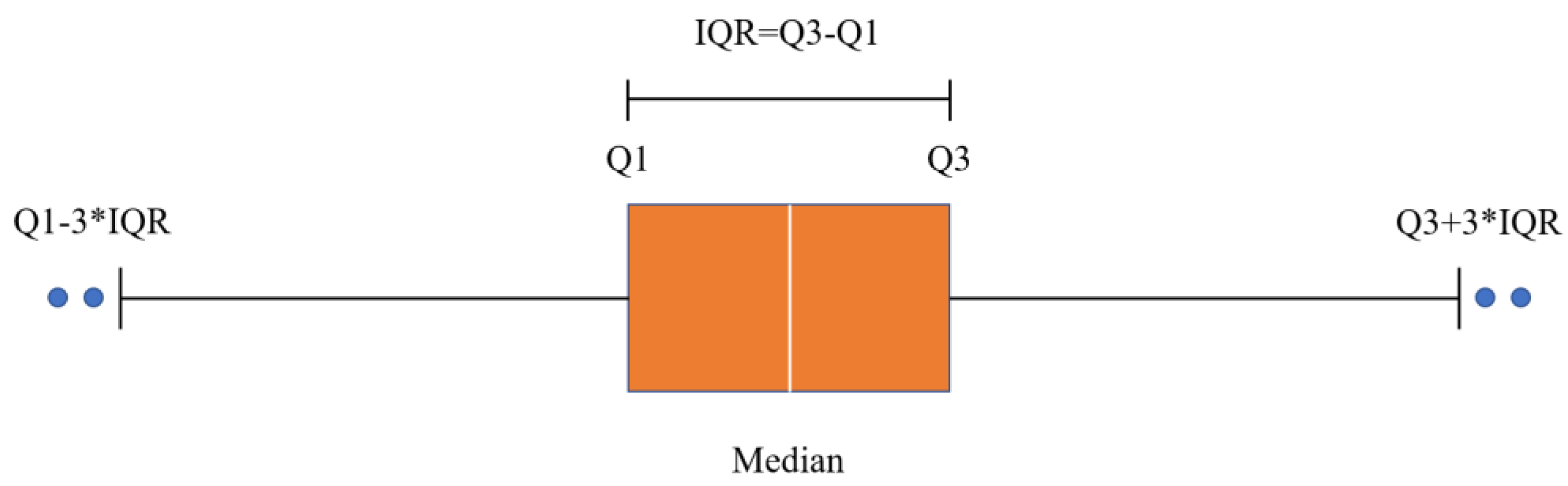
3.3. Quartile Robust Model

In order to reduce the influence of gross errors of observations, robust estimation is usually integrated into Kalman filtering. The variance expansion factor is used before calculation of the matrix gain to adjust the variance of different observations in the observation noise matrix, i.e., to reduce the impact caused due to gross error by adjusting the weights of different observations. The Institute of geodesy and geophysics Ⅲ (IGG Ⅲ) weight function [31] is widely used in the calculation of variance expansion factors due to its advantages such as boundedness, segmentation, continuity, and efficiency. It is divided into three parts: “normal”, “suspicious”, and “abnormal”, based on the error size of the observed value. The “normal” part is not subject to weight adjustment, the “suspicious” part is subject to weight reduction according to (6), and the “abnormal” part is set to zero to eliminate the gross error [32,33], but to avoid calculation problems, we usually set it to ${10}^{-6}$, shown as follows:

$${\lambda }_i=\frac{1}{{\gamma }_i},{\gamma }_i=\left\{\begin{array}{cc}1& w_i<k_0\\ \frac{k_0}{w_i}\times {\left(\frac{k_1-w_i}{k_1-k_0}\right)}^2& k_0<w_i<k_1\\ {10}^{-6}& w_i>k_1\end{array}\right.$$

(6)

where ${\lambda }_i$ is the variance expansion factor, ${\gamma }_i$ is the equivalent weight amplification factor, $w_i$ is the standardized innovation value, and $k_0$ and $k_1$ are constant thresholds, which are generally selected based on experience. As the standardized innovation value can reflect the current epoch observation value relative to the previous epoch state, it can be used to judge the abnormality of the observation value. The value of $w_i$ is determined by the following expression:

$$w_i=\frac{v_i}{{\sigma }_{v_i}}$$

(7)

where $v_i$ is the new interest value, and ${\sigma }_{v_i}$ is the standard deviation of the new interest value in the current epoch.

Let the two observations be $i$ and $j$, respectively, and adjust the measurement noise covariance matrix ${\mathit{R}}_k$ by the variance expansion factor ${\lambda }_k$. This is shown as follows:

$$\left\{\begin{array}{c}{\overline{\mathit{R}}}_{ii}={\lambda }_{ii}*{\mathit{R}}_{ii}\\ {\overline{\mathit{R}}}_{jj}={\lambda }_{jj}*{\mathit{R}}_{jj}\\ {\overline{\mathit{R}}}_{ii}=\sqrt{{\lambda }_{ii}{\lambda }_{jj}}*{\mathit{R}}_{ij}\end{array}\right.$$

(8)

where ${\mathit{R}}_{ii}$ and ${\mathit{R}}_{jj}$ represent the variance of observations $i$ and $j$, respectively, ${\mathit{R}}_{ij}$ is their covariance, ${\lambda }_{ii}$ and ${\lambda }_{jj}$ denote the variance expansion factor of ${\mathit{R}}_{ii}$ and ${\mathit{R}}_{jj}$, respectively, and ${\overline{\mathit{R}}}_{ii}$, ${\overline{\mathit{R}}}_{ii}$ and ${\overline{\mathit{R}}}_{ij}$ are the variance and covariance of the observed values $i$ and $j$ after variance expansion, respectively.

Although conventional robust Kalman filtering can eliminate most gross errors, there are few smartphone observations in the same epoch, and the mean and standard deviation used for data standardization are greatly affected by outliers. Furthermore, $k_0$ and $k_1$ as constant thresholds cannot change according to the quality of overall observations in the current epoch. The quartile method has high calculation efficiency and does not require any prior distribution of data. It discards the part with a large absolute value in a group of data and only uses the values around the data center, which can avoid the impact of abnormal values on the criteria. Therefore, a new method based on the quartile method is proposed to establish a robust model and calculate the variance expansion factor to dynamically determine the threshold value without standardizing the innovation value. The modified expression is as follows:

$${\lambda }_i=\frac{1}{{\gamma }_i},{\gamma }_i=\left\{\begin{array}{cc}1& \left|v_i\right|<{\tilde{k}}_0\\ \frac{{\tilde{k}}_0}{\left|v_i\right|}\times {\left(\frac{{\tilde{k}}_1-\left|v_i\right|}{{\tilde{k}}_1-{\tilde{k}}_0}\right)}^2& {\tilde{k}}_0<\left|v_i\right|<{\tilde{k}}_1\\ {10}^{-6}& \left|v_i\right|>{\tilde{k}}_1\end{array}\right.$$

(9)

where ${\tilde{k}}_0$ and ${\tilde{k}}_1$ are the dynamic thresholds determined by the quartile method, which can be obtained as follows:

$${\tilde{k}}_0=min\left(\left|Q1\right|,\left|Q3\right|\right){\tilde{k}}_1=min\left(\left|Q1-3*IQR\right|,\left|Q3+3*IQR\right|\right)$$

(10)

where $min\left(*\right)$ is the smaller value and $\left|*\right|$ is the absolute value. As the value with a smaller absolute value is closer to the median and closer to the “normal value area”, ${\tilde{k}}_0$ and ${\tilde{k}}_1$ both choose the value with a smaller absolute value.

Figure 1 is the quartile threshold map, where Q1 and Q3 are the upper and lower quartiles, respectively, IQR is the interquartile range, Median denotes the median, Q1—3 * IQR is the upper bound, and Q3 + 3 * IQR is the lower bound.

The variance expansion factor ${\lambda }_i$ is determined according to (9). In (5), the Kalman gain matrix becomes

$${\overline{\mathit{K}}}_k={\mathit{P}}_{k,k-1}{\mathit{H}}^T{\left(\mathit{H}{\mathit{P}}_{k,k-1}{\mathit{H}}^T+{\overline{\mathit{R}}}_k\right)}^{-1}$$

(11)

where ${\overline{\mathit{R}}}_k$ and ${\overline{\mathit{K}}}_k$ are the covariance matrix of measurement noise and the Kalman filter gain matrix after variance expansion, respectively.

3.4. Classification Adaptive Factor Model

For the kinematics model, constant velocity and constant acceleration models are usually used at present. However, in actual situations, objects often do not move at a constant velocity or a constant acceleration. In order to mitigate the effects of error caused by the abnormality of the kinematic model, the adaptive factor $\alpha$ is introduced based on robust Kalman filtering and is applied to the state covariance matrix of the measurement update at time $k$ [34,35,36,37]. This factor is mainly determined by the selection of an adaptive factor model and the construction of state error discriminant statistics.

The classification adaptive factor model divides the state parameters of the object into two categories: position and velocity. It constructs adaptive factors applicable to position and velocity prediction information to control the influence caused by the abnormal position and velocity vectors, respectively [38]. The state error discriminant statistics are used to judge the abnormality of the motion model. Commonly used statistics include state discrepancy statistics, prediction residual statistics, and variance component ratio statistics. The prediction residual may contain errors due to other sources, and the variance component is more complex and inefficient than the statistics. Therefore, the state discrepancy value is utilized as the state error discrimination statistics [39,40]. The method for construction of the position state discrepancy is as follows:

$$∆{\mathit{x}}_{\mathit{k}}=\frac{||{\tilde{\mathit{X}}}_{\mathit{k}}-{\widehat{\mathit{X}}}_{\mathit{k},\mathit{k}-\mathbf{1}}||}{\sqrt{tr\left({\mathit{P}}_{k,k-1}\right)}}k=1,2,3$$

(12)

where $∆{\mathit{x}}_{\mathit{k}}$ represents the position discrepancy statistic, $tr$ is the trace of the matrix, ${\tilde{\mathit{X}}}_{\mathit{k}}$ is the robust solution at the current epoch, and ${\widehat{\mathit{X}}}_{\mathit{k},\mathit{k}-1}$ is the predicted position solution at the current epoch. Similarly, the speed state discrepancy can be constructed as

$$∆{\dot{\mathit{x}}}_{\mathit{k}}=\frac{||{\widetilde{\dot{\mathit{X}}}}_{\mathit{k}}-{\widehat{\dot{\mathit{X}}}}_{\mathit{k},\mathit{k}-\mathbf{1}}||}{\sqrt{tr\left({\mathit{P}}_{k,k-1}\right)}}k=4,5,6$$

(13)

where $∆{\dot{\mathit{x}}}_{\mathit{k}}$ is the speed discrepancy statistic, ${\widetilde{\dot{\mathit{X}}}}_{\mathit{k}}$ is the accurate speed value of the current epoch, and ${\widehat{\dot{\mathit{X}}}}_{\mathit{k},\mathit{k}-\mathbf{1}}$ is the predicted speed value of the current epoch. The value of ${\widetilde{\dot{\mathit{X}}}}_{\mathit{k}}$ can be calculated as follows:

$${\widetilde{\dot{\mathit{X}}}}_{\mathit{k}}=\frac{{\tilde{\mathit{X}}}_{\mathit{k}}-{\mathit{x}}_{\mathit{k}-\mathbf{1}}}{t}$$

(14)

where ${\tilde{\mathit{X}}}_{\mathit{k}}$ is the robust solution at the current epoch, ${\mathit{x}}_{\mathit{k}-\mathbf{1}}$ is the estimated position at the previous epoch, and $t$ is the sampling interval.

Similarly, the IGG Ⅲ weight function is used to calculate the position and speed adaptive factors, shown as follows:

$$\alpha =\left[\begin{array}{ccccc}{\alpha }_P& & & & \\ & {\alpha }_V& & & \\ & & 1& & \\ & & & \ddots & \\ & & & & 1\end{array}\right]$$

(15)

where $\alpha$, ${\alpha }_P$, and ${\alpha }_V$ denote the classification, position, and speed adaptive factor matrices, respectively.

The discrepancy values of position and speed states are used as the discriminant statistics. After determining the adaptive factor through the classification adaptive factor model, the prediction error covariance matrix in (5) is changed to

$${\overline{\mathit{P}}}_{k,k-1}=\frac{1}{\alpha }\left({\mathit{A}}_{k,k-1}{\mathit{P}}_{k-1}{\mathit{A}}_{k,k-1}^T+{\mathit{Q}}_{k-1}\right)$$

(16)

where ${\overline{\mathit{P}}}_{k,k-1}$ is the prediction covariance matrix adjusted by the adaptive factor.

4. Experiments and Results Analysis

An Huawei P40 and Xiaomi 8 were used for dynamic simulation and dynamic tests, respectively, in order to verify the effectiveness of the robust adaptive algorithm and analyze the dynamic positioning performance of Android smartphones. As the duty cycle mechanism will cause discontinuous carrier phase observations, the Xiaomi 8 actively turns off the duty cycle mechanism, while the Huawei P40 turns off the duty cycle mechanism by default. Six groups of data were collected in the experiment. Three groups of static data and three groups of dynamic data were solved in dynamic mode.

Table 2. Data collection content and strategy.

Solution Mode	Baseline Code	Sampling Interval/s	Sampling Duration/h	Collection Environment	Acquisition Mode	Baseline Length/km
Simulated dynamics	S1	1	3.34	tree shelter	static	0.07
	S2	1	2.66	broad road	static	1.10
	S3	1	2.01	broad square	static	9.00
Dynamic	D1	1	0.45	tree shelter	walk	1.40 (farthest)
	D2	1	0.48	tree shelter	trolley	0.08 (farthest)
	D3	1	0.66	broad road	vehicle	2.87 (farthest)

provides the specific data collection contents and strategies.

4.1. Simulated Dynamic Test

The simulated dynamic test data were collected by the Xiaomi 8 and Huawei P40 on 10 July, 2 July, and 11 July 2022. The sampling interval was 1 s; the sampling durations were 3.34 h, 2.66 h, and 2.01 h; the baseline lengths were 68 m, 1.1 km, and 9 km, respectively. For the convenience of subsequent expression, the three groups of data were denoted as S1, S2, and S3. The three groups of data were processed using the four-system single-frequency GPS (L1) + GLO (R1) + GAL (E1) + BDS-3 (B1I).

Table 3. Calculation strategy of simulated dynamic experiment.

Content	Method
Solution mode	GPS(L1) + GLO(R1) + GAL(E1) + BDS-3(B1I)
Ephemeris	Broadcast ephemeris
Ionospheric model	Klobuchar
Tropospheric model	Saastamoinen
Stochastic model	elevating angle and uncertainty
Parameter estimation model	Robust Kalman filtering
Pretreatment rules	ELE < 15°, SNR < 20 dB, Uncertainty > 0.1

shows the specific solution strategy. In the data preprocessing phase, the experiment eliminated satellites with an elevating angle less than 15 degrees, a signal-to-noise ratio less than 20 dB, and an uncertainty greater than 0.1.

Figure 2 shows the surrounding environment of S1, S2, and S3 smartphone rover stations from left to right. Figure 3a–c show the tracking satellite of S1, S2, and S3 smartphone rover stations, respectively. Figure 3d–f represent the changes in position dilution of precision (PDOP) values of S1, S2, and S3 baselines, respectively, under the four-system solution mode. In Figure 3, the red and blue colors represent the relevant contents of the Xiaomi 8 and Huawei P40.

Table 4. Statistics of effective satellite numbers and PDOP values.

Baseline Code	Mobile Phone Type	Effective Satellites			PDOP
		Max	Min	Ave	Max	Min	Ave
S1	Xiaomi 8	14	5	10.7	2.55	1.32	1.68
	Huawei P40	21	2	14.3	2.21	1.04	1.28
S2	Xiaomi 8	20	7	16.5	1.96	1.08	1.22
	Huawei P40	22	13	19.1	1.77	1.01	1.19
S3	Xiaomi 8	22	11	16.7	2.12	1.06	1.31
	Huawei P40	23	11	19.6	1.69	0.91	1.13

shows the specific statistical information of S1, S2, and S3 baseline Xiaomi 8 and P40 tracking satellites and PDOP values.

The following observations can be made from Figure 3a–c and Table 4:

(1)

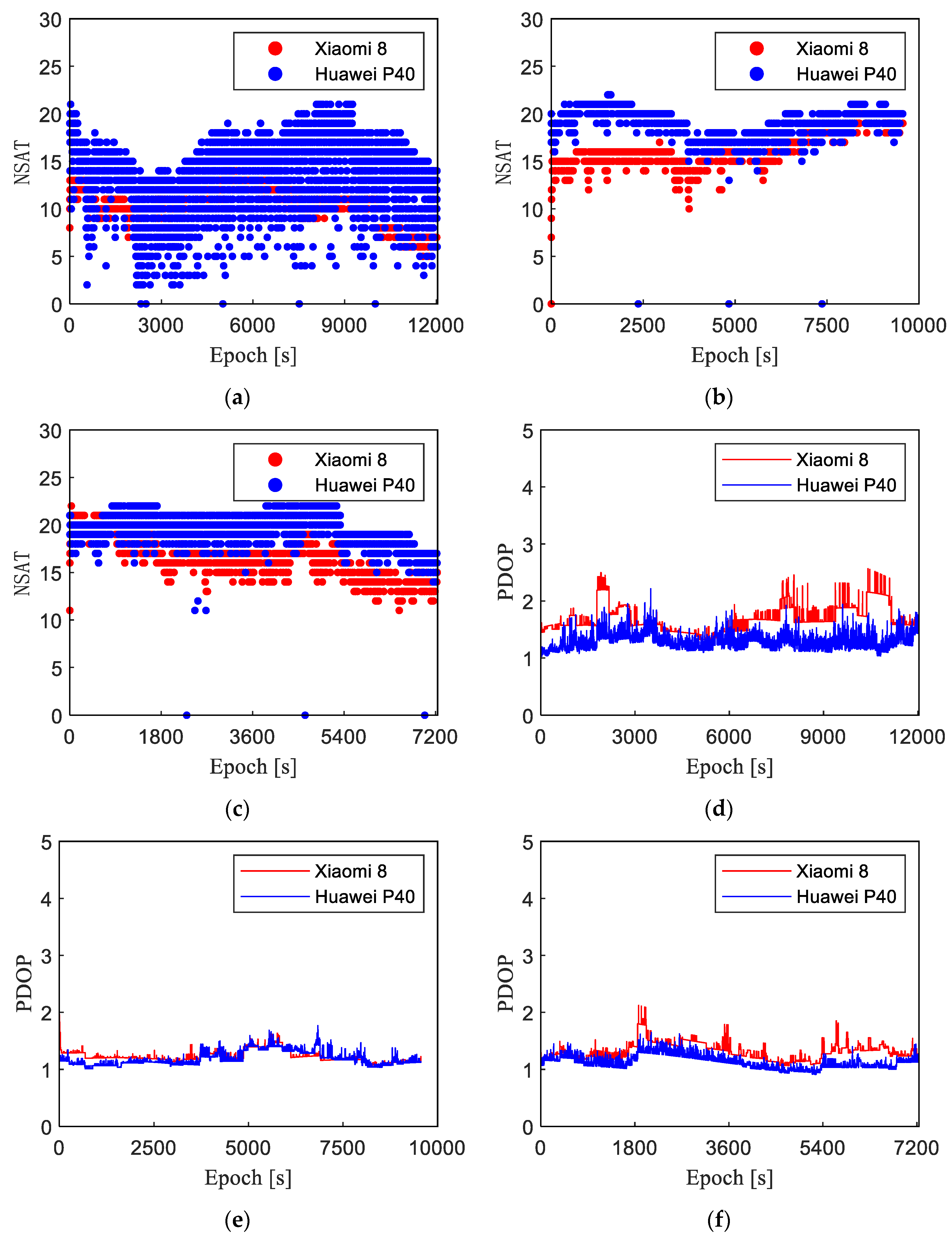
On average, the Huawei P40 can receive signals from 14.3, 19.1, and 19.6 satellites, and the Xiaomi 8 can receive signals from 10.7, 16.5, and 16.7 satellites. Compared with the latter, the former can track 3–4 more satellites, mainly BDS-3 satellites. This is due to a problem in the design of the hardware signal channel of the Xiaomi 8.

(2)

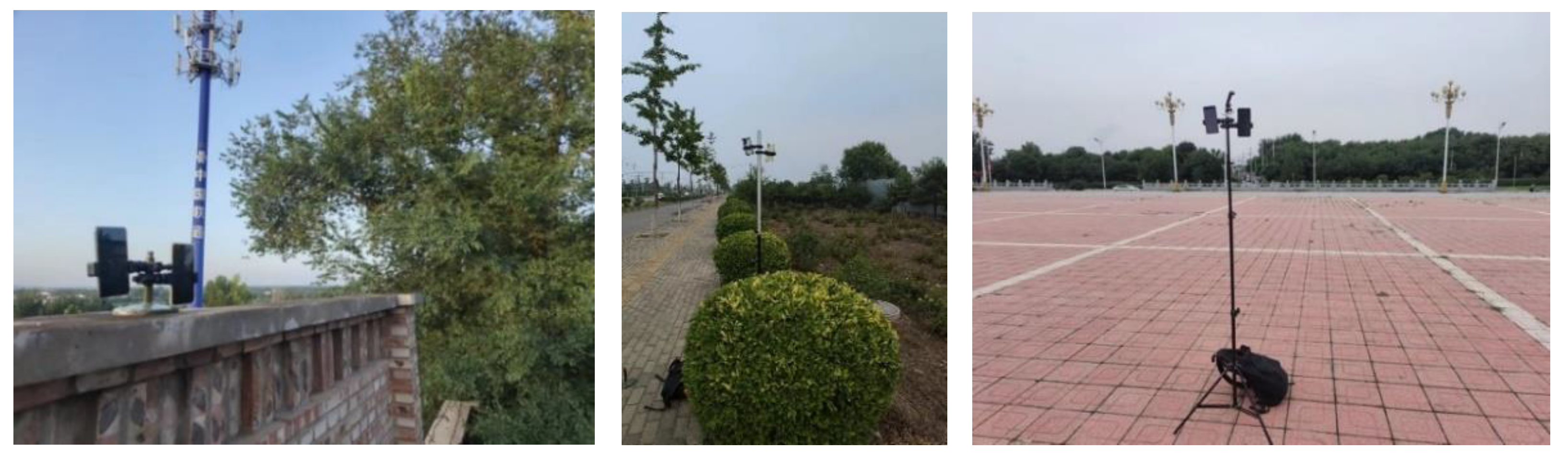
Although the Huawei P40 captures signals from a large number of satellites, most satellites in the sheltered environment (S1) are frequently locked and unlocked alternately. This behavior is mainly related to the antenna layout inside the smartphone and the hardware, such as the internal loop tracker. In a good environment (S2, S3), the Huawei P40 exhibits a stable tracking of more satellites than the Xiaomi 8, providing better satellite geometry.

(3)

The PDOP is an important index to measure the satellite positioning accuracy. Generally, a PDOP value of less than 3 is considered to indicate a good satellite spatial geometric distribution. It can be observed from Figure 3d–f and Table 4 that the change trend of the PDOP value is consistent with the number of satellites. As the Huawei P40 can capture signals from a higher number of satellites, the PDOP value is small. However, due to its poor ability to lock satellites in a sheltered environment, the value shows strong fluctuations, which will affect the positioning results.

In summary, the Huawei P40 captures signals from a higher number of satellites than the Xiaomi 8 and has a relatively small PDOP value. However, its stability is poorer compared to that of the Xiaomi 8; therefore, the positioning accuracy will be affected in sheltered environmental conditions.

Four-system single-frequency (L1 + R1 + E1 + B1) RTK calculation experiments were conducted using the measured baseline data of S1, S2, and S3 with different lengths and different environments. Compared with conventional RTK, robust RTK adds a quartile robust model that conforms to the characteristics of smartphone data, which can reasonably determine the weights of observation data from different satellites. Next, the conventional RTK mode and robust RTK mode were compared and analyzed with respect to convergence speed and positioning accuracy, and the positioning performance of the Xiaomi 8 and P40 single-frequency RTK algorithm was evaluated.

Figure 4, Figure 5 and Figure 6 show the positioning deviation diagram corresponding to baseline data of S1, S2, and S3 of the Xiaomi 8 in three directions of E/N/U under the conventional RTK and robust RTK positioning methods. Figure 7, Figure 8 and Figure 9 show the positioning deviation diagram of the Huawei P40 for S1, S2, and S3 baselines in E/N/U directions under the conventional RTK and robust RTK positioning methods.

Table 5. RMS values, lifting ratios, and convergence times in E/N/U directions for Xiaomi 8 under simulated dynamic conditions.

Baseline Code	Solution Mode	RMS			Planar Accuracy/m	Overall Accuracy/m	Convergence Time/s
		E/m	N/m	U/m
S1	Conventional	0.547	1.306	4.836	1.416	5.039	-
	Robust	0.188	0.113	0.266	0.219	0.345	74
	Lifting ratio	65.6%	91.3%	94.5%	84.5%	93.1%	-
S2	Conventional	9.644	4.08	6.244	10.471	12.192	-
	Robust	0.234	0.123	0.361	0.264	0.448	236
	Lifting ratio	97.6%	97.0%	94.2%	97.5%	96.3%	-
S3	Conventional	1.634	0.498	0.82	1.708	1.895	-
	Robust	0.108	0.186	0.177	0.215	0.279	134
	Lifting ratio	93.4%	62.7%	78.4%	87.4%	85.3%	-

shows the RMS positioning results, convergence times, and lifting ratios of the Xiaomi 8 in the E/N/U directions.

Table 6. RMS values, lifting ratios, and convergence times in E/N/U directions for Huawei P40 under simulated dynamic conditions.

Baseline Code	Solution Mode	RMS			Planar Accuracy m	Overall Accuracy/m	Convergence Time/s
		E/m	N/m	U/m
S1	Conventional	0.579	0.785	1.084	0.975	1.458	417
	Robust	0.365	0.374	0.611	0.523	0.804	119
	Lifting ratio	36.9%	52.4%	43.6%	46.4%	44.8%	71.5%
S2	Conventional	0.136	0.227	0.178	0.265	0.319	211
	Robust	0.077	0.149	0.121	0.168	0.207	54
	Lifting ratio	43.4%	34.4%	32.0%	36.6%	35.2%	74.4%
S3	Conventional	0.161	0.091	0.26	0.185	0.319	415
	Robust	0.104	0.058	0.198	0.119	0.231	288
	Lifting ratio	35.4%	36.3%	23.8%	35.7%	27.6%	30.6%

shows the RMS positioning results, convergence times, and lifting ratios of the Huawei P40 in the E/N/U directions.

We determine the convergence standard as a deviation of less than 0.5 m for 60 consecutive epochs in three directions of E/N/U. This is mainly because the smartphone antenna and GNSS chipsets are of poor quality, the pseudo-range observation contains many gross errors, and the conventional RTK cannot reasonably assign weights to them. These reasons cause the Kalman filtering system to be unstable and the ambiguity to seriously deviate from the true value, and from Figure 4, Figure 5 and Figure 6 and Table 5, we can make the following conclusions:

(1)

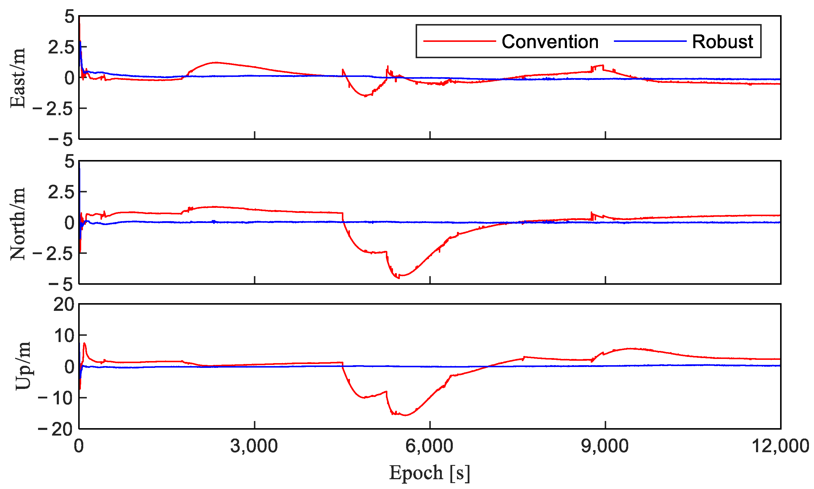
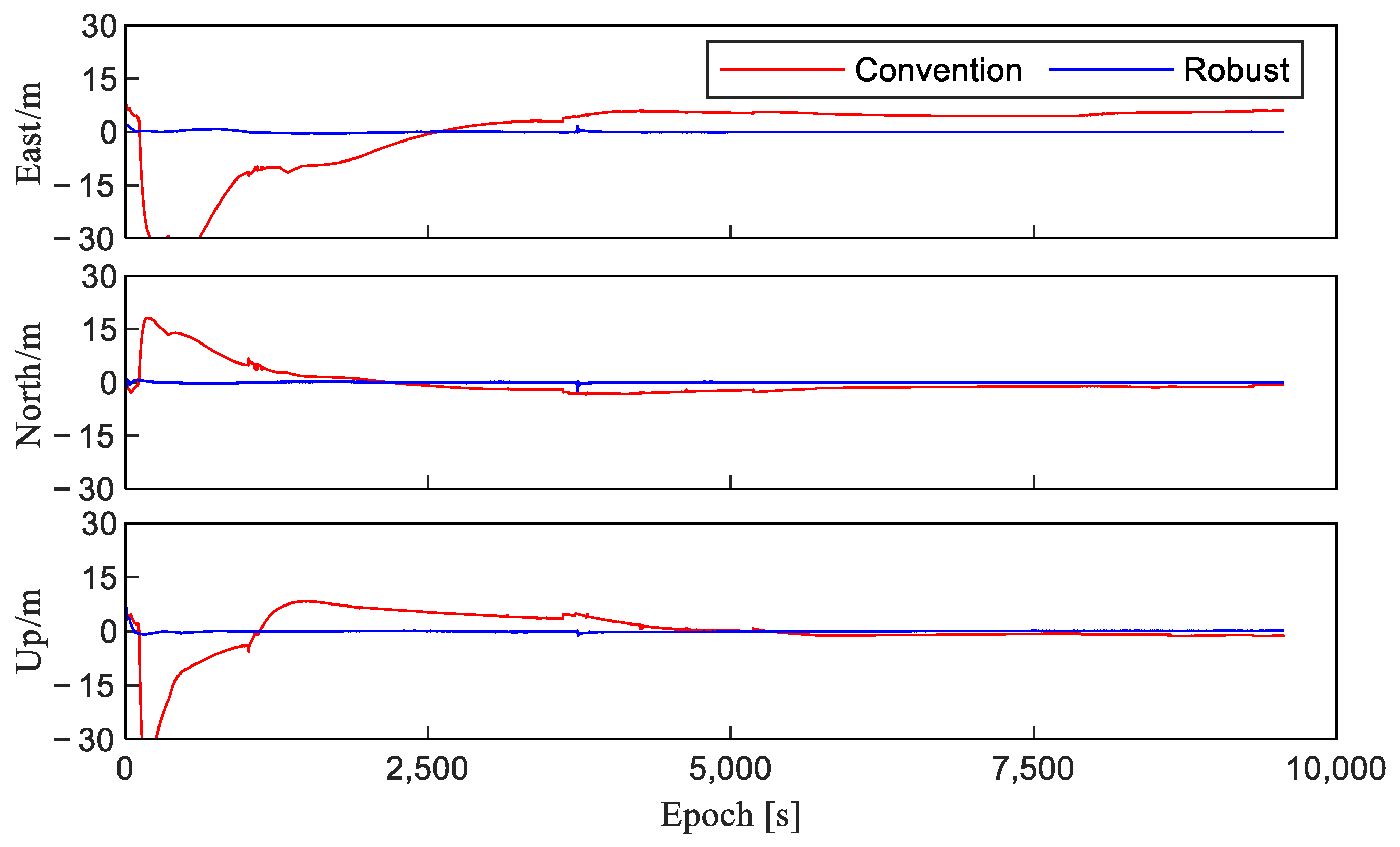
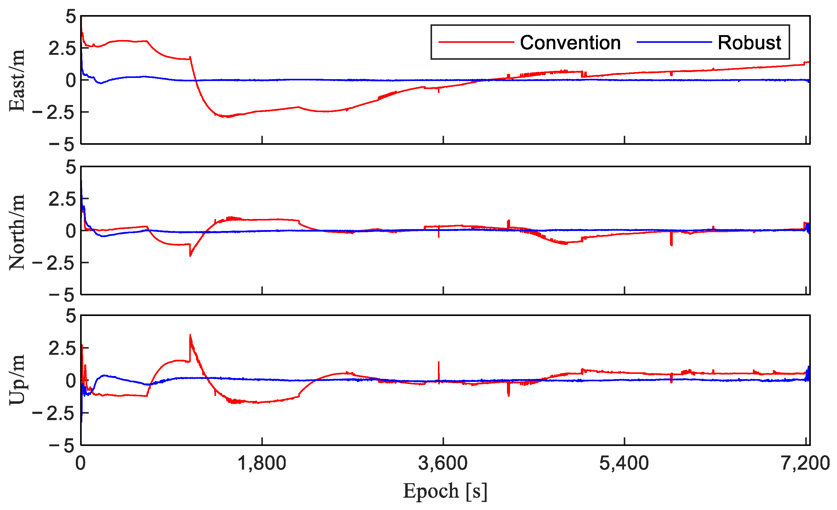
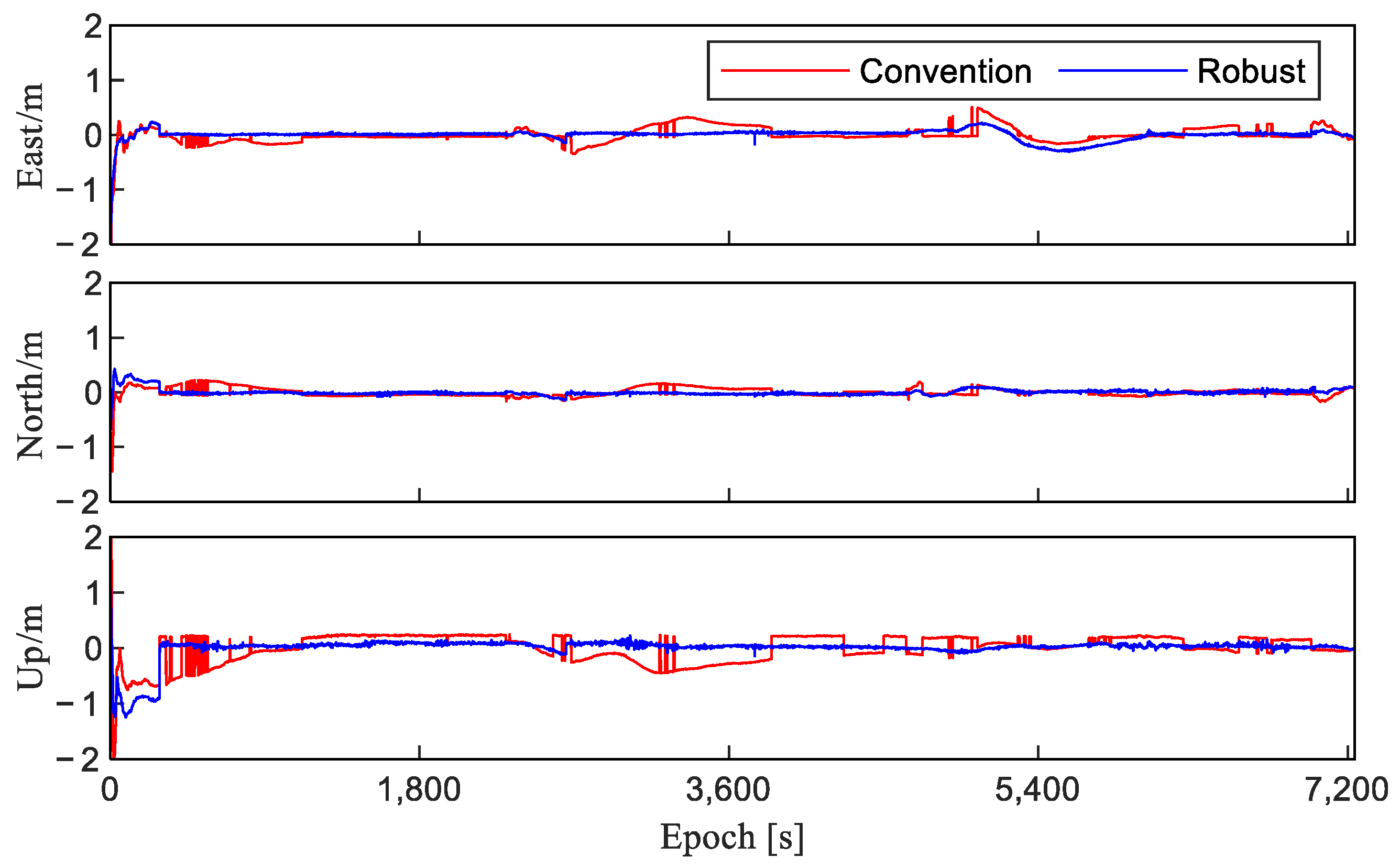
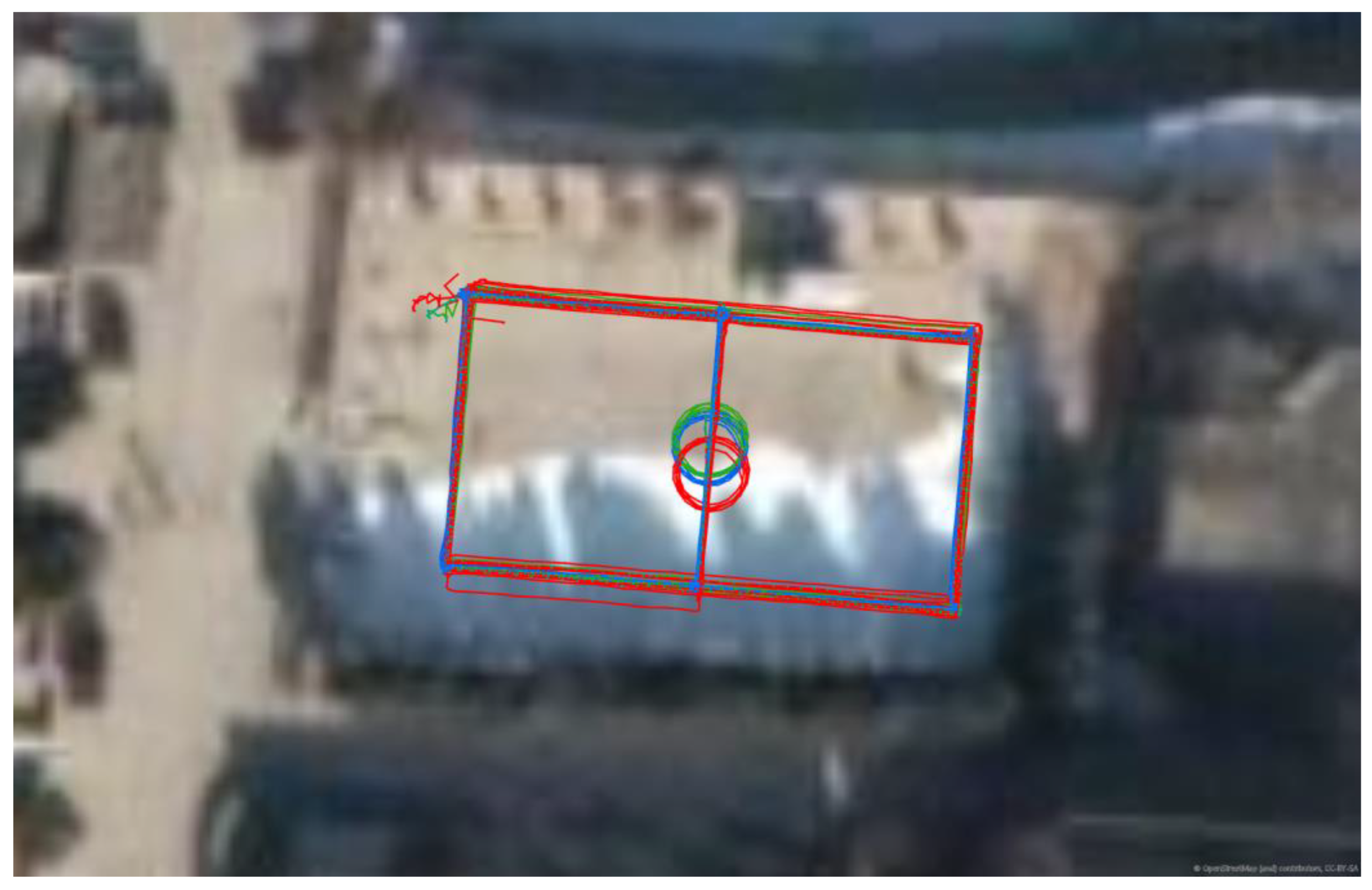
The Xiaomi 8 cannot converge in the conventional four-system single-frequency RTK solution mode. The robust RTK with the quartile model can eliminate large gross errors and reasonably allocate the weights to the observation values according to the robust weight function. This results in the improvement of its convergence speed and positioning accuracy.

(2)

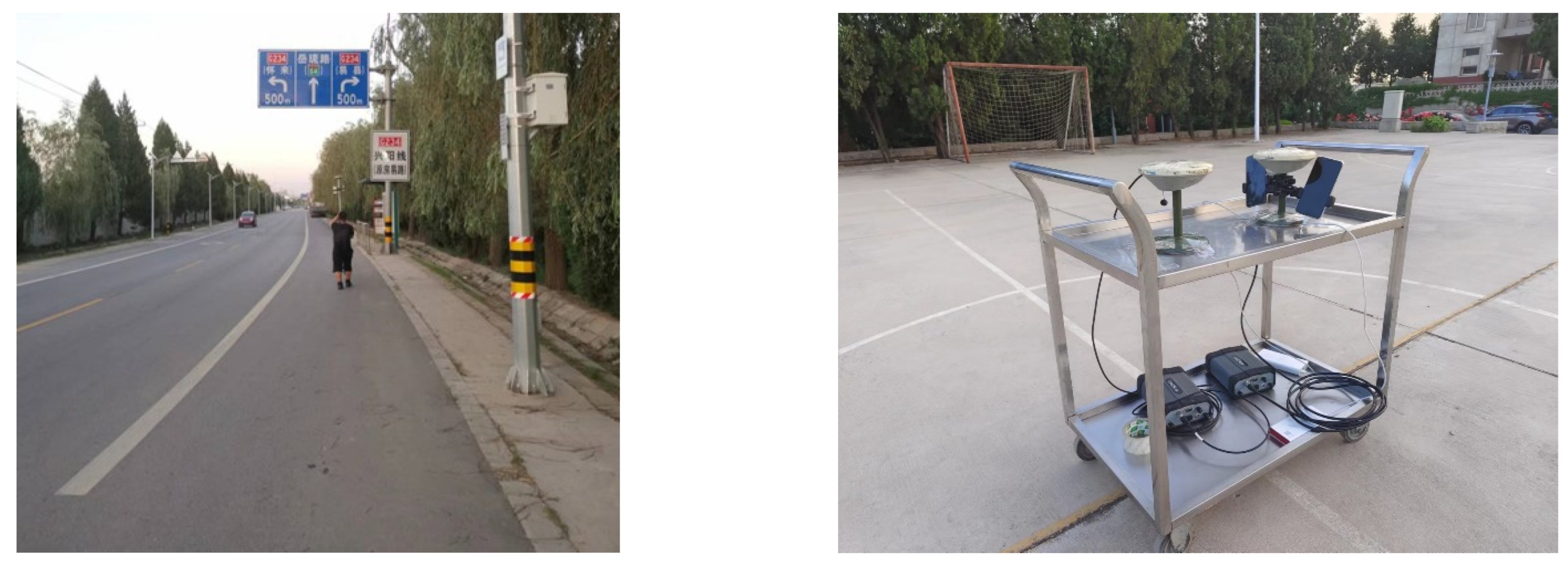
The S1 baseline is an environment where half the sky is sheltered by trees, while S2 and S3 are open-roadside and open-square environments, respectively. However, under the robust RTK solution mode, the baseline planar accuracy of the Xiaomi 8 under S1, S2, and S3 can be kept within 0.3 m, and the elevation positioning accuracy is kept within 0.5 m. As a result, the overall positioning accuracy is significantly improved by more than 85%. This is because the quartile model effectively eliminates gross errors and reasonably assigns weights to observations of different quality, which improves the positioning accuracy.

The following conclusions can be obtained from Figure 7, Figure 8 and Figure 9 and Table 6:

In the robust RTK solution mode, the planar and elevation accuracies of the Huawei P40 under S2 and S3 baseline conditions are maintained within 0.2 m. The overall positioning accuracy remains within 0.3 m, which is higher than that of Xiaomi 8. This is because the Huawei P40 can receive signals from a higher number of satellites, providing better satellite geometric spatial structure and more redundant data. The planar positioning and overall accuracies are improved by more than 35% and 25%, respectively, which effectively improves the convergence speed and positioning accuracy. Compared with S2 and S3 baseline solution results, the Huawei P40 has planar and elevation positioning accuracies of 0.523 m and 0.611 m, respectively, under the S1 baseline, which are significantly lower. This is because the Huawei P40 has poor satellite tracking and locking capabilities, and the number of satellites whose signals can be received fluctuates severely in a sheltered environment. This causes a frequent reset of ambiguity parameters and an inability to calculate positioning results with a high accuracy.

4.2. Dynamic Test

The dynamic test data were collected by a Xiaomi 8 on 12 March, 22 May, and 24 June 2022. The sampling interval was 1 s, and the sampling durations were 0.66 h, 0.48 h, and 0.45 h, respectively. The modes used for data collection were walking on the road, trolley on the basketball court, and vehicle on the road. For the sake of convenience of subsequent expressions, the three groups of data were recorded as D1, D2, and D3, respectively. The three groups of data were processed using the four-system single-frequency GPS (L1) + GLO (R1) + GAL (E1) + BDS-3 (B1). As the observation value received by the Huawei P40 is interrupted many times and is obviously abnormal, the dynamic experiment did not process the relevant data of the Huawei P40.

Table 7. Calculation strategy of dynamic experiment.

Content	Method
Solution mode	GPS (L1) + GLO (R1) + GAL (E1) + BDS-3 (B1I)
Ephemeris	Broadcast ephemeris
Ionospheric model	Klobuchar
Tropospheric model	Saastamoinen
Stochastic model	Altitude angle and uncertainty
Parameter estimation model	Robust adaptive Kalman filtering
Content	Method
Pretreatment rules	ELE < 15°, SNR < 20 dB, Uncertainty > 0.1

shows the specific solution strategy.

Figure 10 shows the specific test scenario of D1, D2, and D3 dynamic data measurements. CHC P5 is a high-precision GNSS receiver, and its positioning accuracy is far higher than that of smartphones. Therefore, the Xiaomi 8 is fixed on the side of the antenna sucker connected with the CHC P5 receiver to jointly conduct dynamic data acquisition and acquire the receiver solution results as the true values. Figure 11, Figure 12 and Figure 13 show the D1 walking dynamic track, D2 trolley dynamic running track, and D3 vehicle dynamic running track. Figure 14 and Figure 15 show the turning and straight-line details for the D1 walking dynamic track and D3 vehicle dynamic track, respectively. In these figures, blue, red, and green represent the reference track of the CHC P5 receiver, normal RTK operation track, and robust adaptive RTK operation track, respectively.

Table 8. RMS values and lifting ratios in dynamic E/N/U directions.

Baseline Code	Solution Mode	RMS			Planar Accuracy/m	Overall Accuracy/m
		E/m	N/m	U/m
D1	Conventional	1.765	1.443	2.173	2.28	3.15
	Robust adaptation	0.828	1.22	1.851	1.474	2.085
	Lifting ratio	53.1%	15.5%	14.8%	35.4%	33.8%
D2	Conventional	0.458	0.549	1.034	0.715	1.257
	Robust adaptation	0.345	0.285	0.944	0.447	1.045
	Lifting ratio	24.7%	48.1%	8.7%	37.5%	16.9%
D3	Conventional	0.637	0.656	2.067	0.914	2.26
	Robust adaptation	0.603	0.49	1.679	0.777	1.85
	Lifting ratio	5.3%	25.3%	18.8%	15.0%	18.1%

shows the dynamic RMS values and lifting ratios of the Xiaomi 8 in E/N/U directions.

The following conclusions can be obtained from Figure 11, Figure 12, Figure 13, Figure 14 and Figure 15:

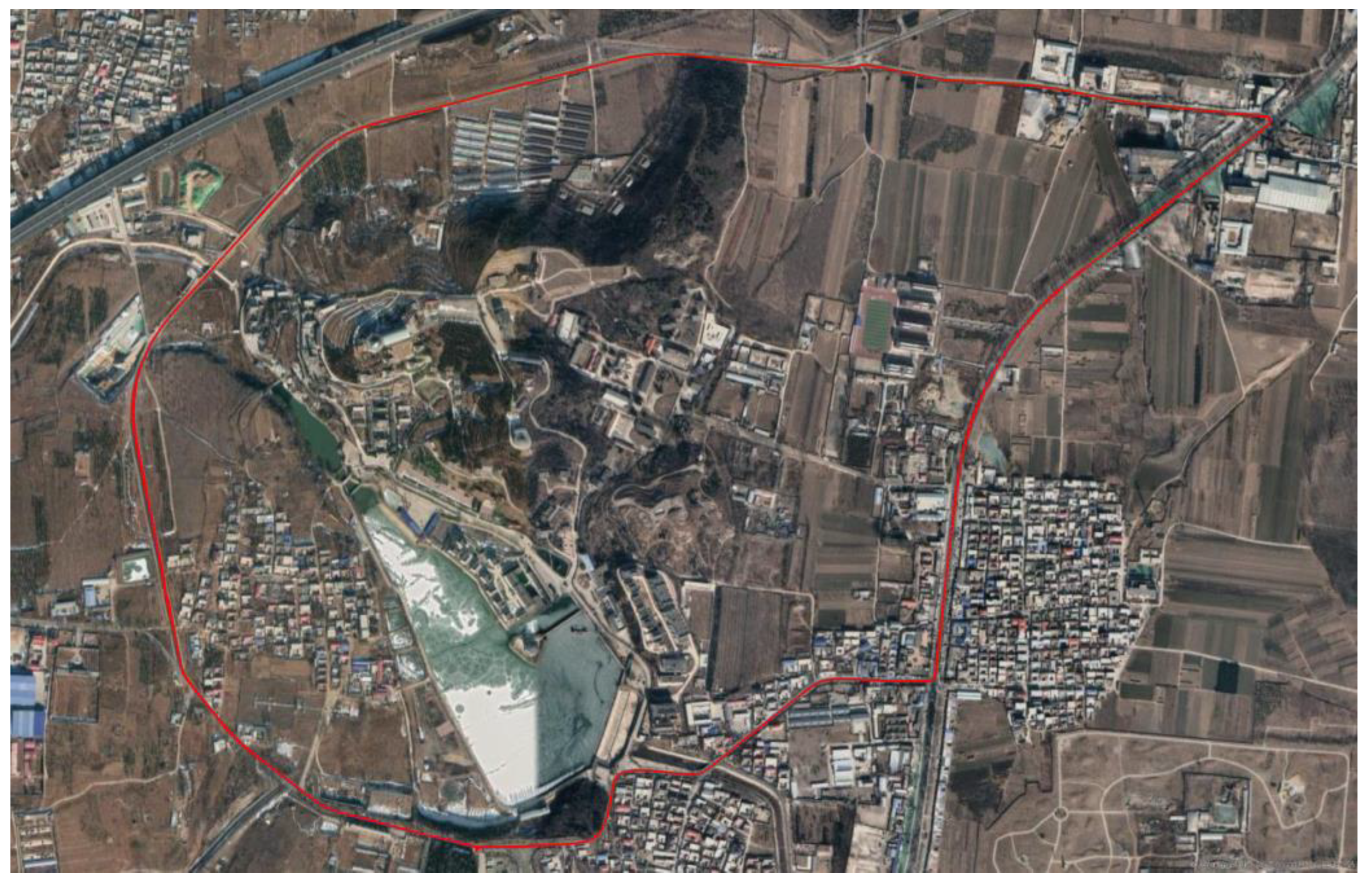
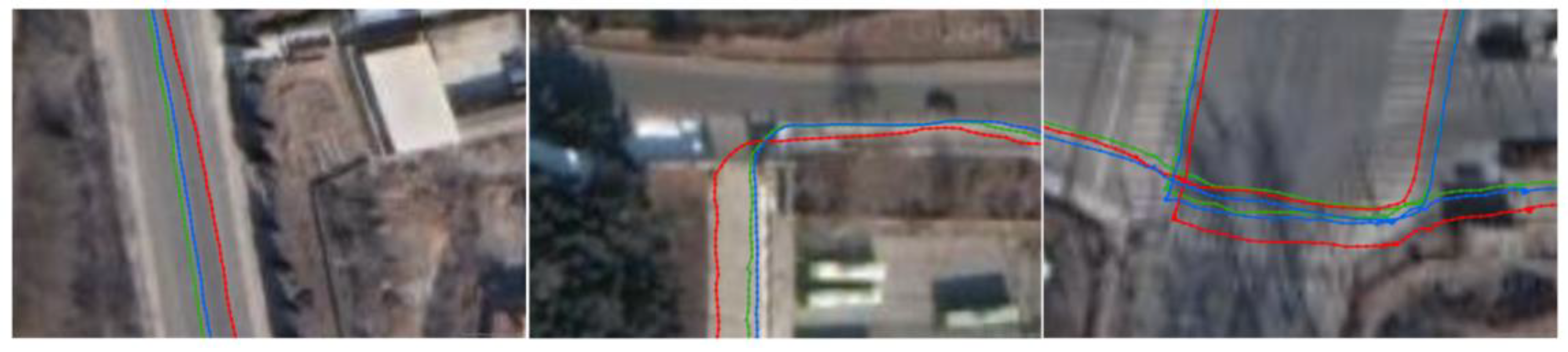
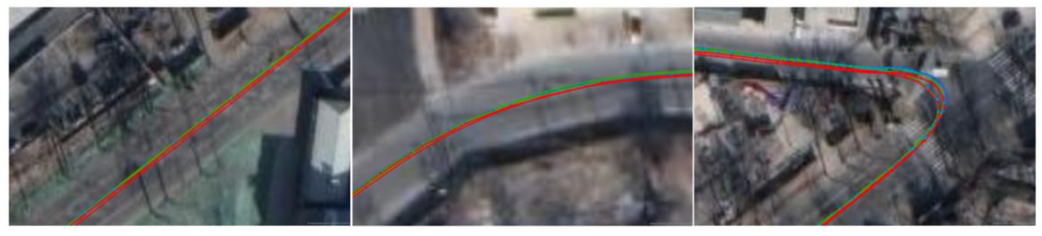
(1)

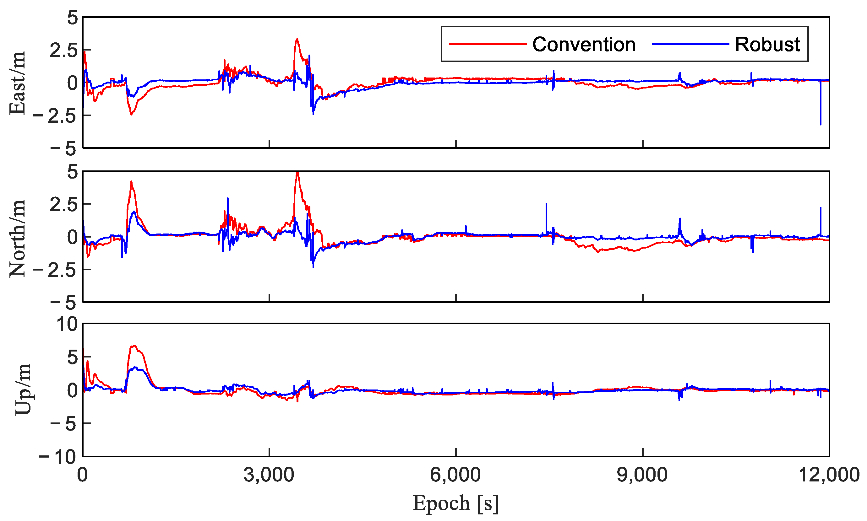
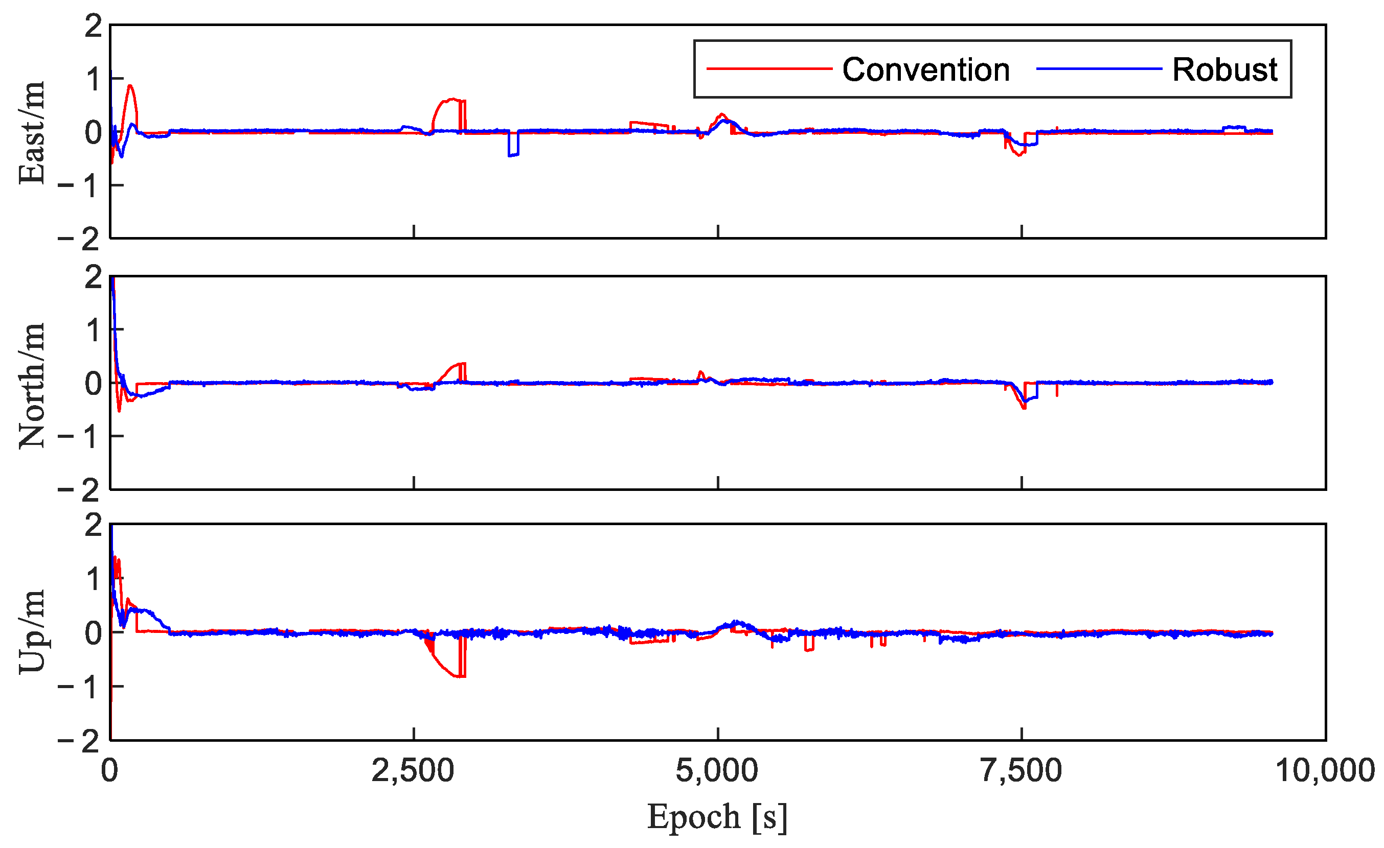
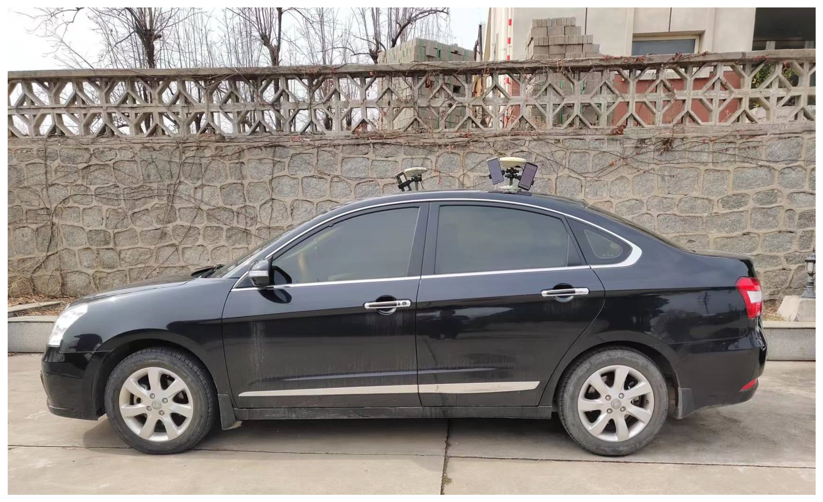
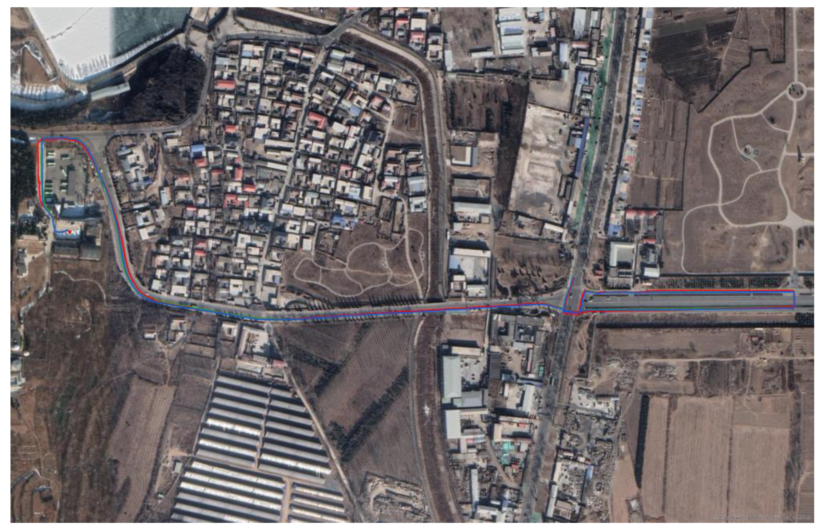
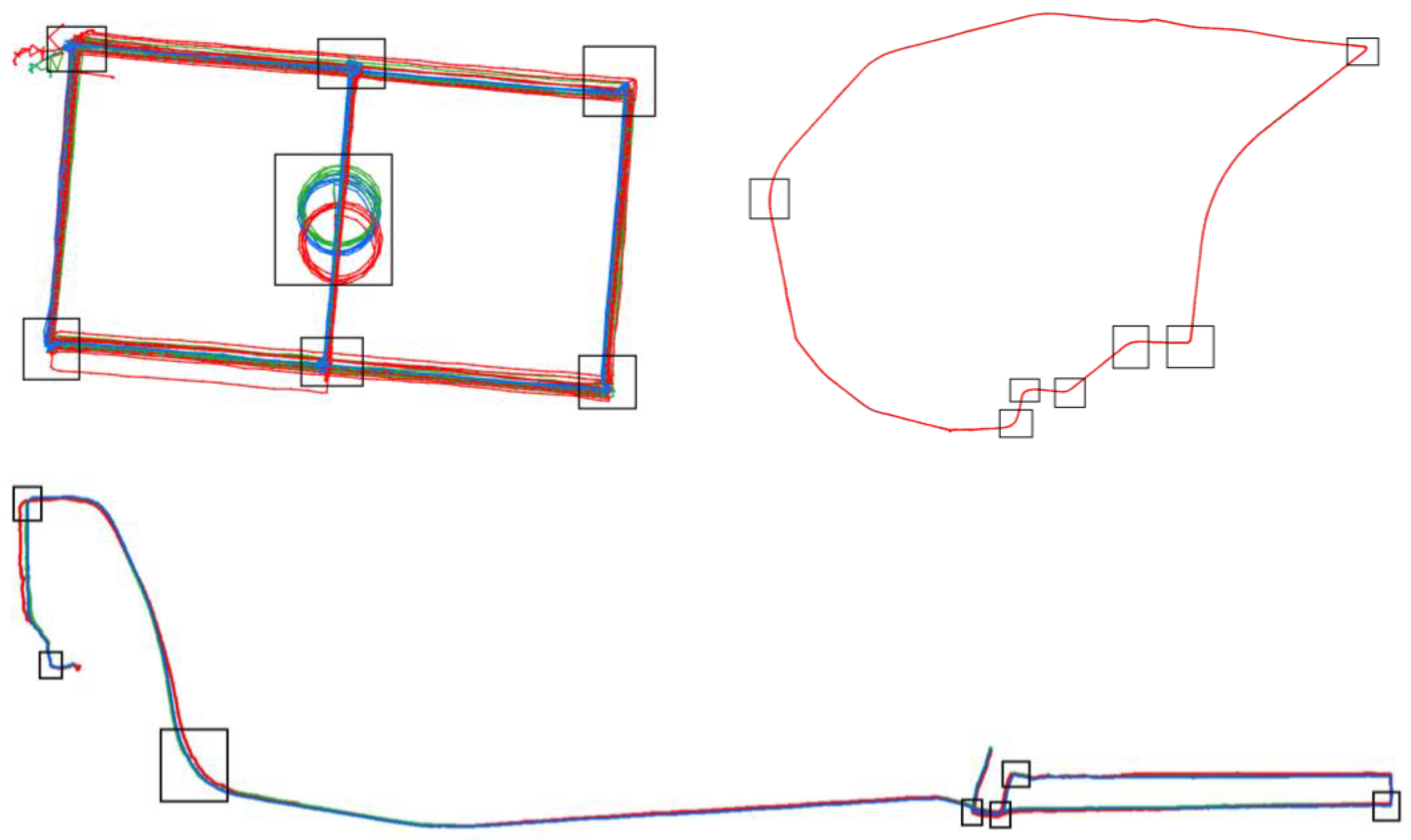
Compared to the solution results obtained using the CHC P5 receiver as a reference, the dynamic trajectory of the red conventional RTK solution results deviates significantly. This deviation is particularly obvious in the turning section because the Kalman filter suffers from hysteresis when there is a sudden motion state change. Consequently, the weight relationship between the predicted and measured values cannot be adjusted in a timely manner. On the other hand, the deviations between the green robust adaptive RTK solution results and the reference track of CHC P5 are small for straight or turning sections, and the track is obviously better. This is because the adaptive model can determine the adaptive factor according to the discriminant statistics, reasonably adjust the weight relationship between the predicted and measured values in a timely manner, and improve the impact caused by the lag of the Kalman filter to a certain extent.

(2)

The planar accuracies of D1, D2, and D3 dynamic data from the Xiaomi 8 in the robust adaptive RTK solution mode are 1.474 m, 0.447 m, and 0.777 m, respectively. The corresponding elevation accuracies are 1.851 m, 0.944 m, and 1.679 m, respectively. The overall positioning accuracies increase by 33.8%, 16.9%, and 18.1%, respectively.

Compared with D2 and D3, the low accuracy of the D1 dynamic data solution is caused by the high elevation difference at the beginning, the serious occlusion of the subsequent road sections, and the large gross errors in the observed values. Therefore, the improvement ratio of the overall positioning accuracy is larger than the former two. The effectiveness of the adaptive model is determined by selecting some nodes with large motion state changes from D1, D2, and D3 dynamic data for accuracy statistics and analysis. Figure 16 shows the map of D1, D2, and D3 dynamic track node selection position markers. Each black box selects 10 consecutive node coordinates for precision statistics.

Table 9. RMS values and lifting proportions of dynamic key nodes in E/N/U directions.

Baseline Code	Solution Mode	RMS			Planar Accuracy /m	Overall Accuracy/m
		E/m	N/m	U/m
D1	Conventional	2.979	1.875	3.835	3.521	5.206
	Robust adaptation	0.712	1.204	1.286	1.399	1.900
	Lifting ratio	76.1%	35.8%	66.5%	60.3%	63.5%
D2	Conventional	0.186	0.590	0.797	0.619	1.009
	Robust adaptation	0.101	0.268	0.554	0.286	0.624
	Lifting ratio	45.6%	54.6%	30.5%	53.7%	38.2%
D3	Conventional	0.342	0.380	1.786	0.511	1.858
	Robust adaptation	0.169	0.113	1.428	0.203	1.443
	Lifting ratio	50.7%	70.4%	20.0%	60.3%	22.4%

shows the specific accuracy statistics and lifting proportions of some nodes of the dynamic track.

It can be observed from Figure 16 and Table 8 and Table 9 that the planar positioning accuracies of the robust adaptive RTK for key nodes of D1, D2, and D3 dynamic data are 1.339 m, 0.286 m, and 0.203 m, respectively, and the elevation positioning accuracies are 1.286 m, 0.554 m, and 1.428 m, respectively. The planar and elevation accuracies and the lifting ratios are better than the results obtained using the full-time solution. The adaptive model can effectively reduce the position error caused by the abnormal kinematics model, which proves its effectiveness.

5. Conclusions

In this study, a robust adaptive RTK positioning algorithm was proposed, which added robust adaptive models to the conventional RTK positioning model in order to provide continuous and accurate dynamic positioning results. The key models in the proposed algorithm were discussed, including the GNSS RTK positioning model, quartile robust model, and adaptive model using the classification adaptive factor. The algorithm was validated using simulated and actual dynamic experiments, where the latter were carried out in open and sheltered environments. The simulated dynamic test results showed that compared with the Xiaomi 8, the Huawei P40 could capture more satellites, but had a weaker satellite locking ability and poor stability. The proposed quartile robust RTK algorithm could effectively eliminate large gross errors, and reasonably allocate weights to different observations according to the innovation vector. It could also improve the overall positioning accuracies of the Xiaomi 8 and Huawei P40 by more than 80% and 25%, respectively. The dynamic experiment results showed that the applied classification adaptive factor model could significantly reduce the error caused by the kinematic model, especially when there were significant changes in the motion state. It can be gathered from the full-time solution results that the overall positioning accuracies in the occluded and open environments improved by more than 30% and 15%, respectively. In conclusion, the algorithm can provide a reference for obtaining continuous and accurate dynamic positioning results.

References

- Magiera, W.; Vārna, I.; Mitrofanovs, I.; Silabrieds, G.; Krawczyk, A.; Skorupa, B.; Apollo, M.; Maciuk, K. Accuracy of Code GNSS Receivers under Various Conditions. Remote Sens. 2022, 14, 2615. [Google Scholar] [CrossRef]
- Ye, J.; Li, Y.; Luo, H.; Wang, J.; Chen, W.; Zhang, Q. Hybrid Urban Canyon Pedestrian Navigation Scheme Combined PDR.; GNSS and Beacon Based on Smartphone. Remote Sens. 2019, 11, 2174. [Google Scholar] [CrossRef]
- Fortunato, M.; Ravanelli, M.; Mazzoni, A. Real-Time Geophysical Applications with Android GNSS Raw Measurements. Remote Sens. 2019, 11, 2113. [Google Scholar] [CrossRef]
- Håkansson, M. Characterization of GNSS observations from a Nexus 9 Android tablet. GPS Solut. 2018, 23, 21. [Google Scholar] [CrossRef]
- Humphreys, T.E.; Murrian, M.; van Diggelen, F.; Podshivalov, S.; Pesyna, K.M. On the feasibility of cm-accurate positioning via a smartphone’s antenna and GNSS chip. In Proceedings of the 2016 IEEE/ION Position, Location and Navigation Symposium (PLANS), Savannah, GA, USA, 11–14 April 2016; pp. 232–242. [Google Scholar] [CrossRef]
- Li, W.; Zhu, X.; Chen, Z.; Dai, Z.; Li, J.; Ran, C. Code multipath error extraction based on the wavelet and empirical mode decomposition for Android smart devices. GPS Solut. 2021, 25, 91. [Google Scholar] [CrossRef]
- Wanninger, L.; Heßelbarth, A. GNSS code and carrier phase observations of a Huawei P30 smartphone: Quality assessment and centimeter-accurate positioning. GPS Solut. 2020, 24, 64. [Google Scholar] [CrossRef]
- Bakuła, M.; Uradziński, M.; Krasuski, K. Performance of DGPS Smartphone Positioning with the Use of P(L1) vs. P(L5) Pseudorange Measurements. Remote Sens. 2022, 14, 929. [Google Scholar] [CrossRef]
- Gao, C.; Chen, B.; Liu, Y. Android smartphone GNSS high-precision real-time dynamic positioning. Acta Geod. Ecartographica Sin. 2021, 50, 18–26. [Google Scholar] [CrossRef]
- Li, Z.; Wang, L.; Wang, N.; Li, R.; Liu, A. Real-time GNSS precise point positioning with smartphones for vehicle navigation. Satell. Navig. 2022, 3, 19. [Google Scholar] [CrossRef]
- Li, M.; Lei, Z.; Li, W.; Jiang, K.; Huang, T.; Zheng, J.; Zhao, Q. Performance Evaluation of Single-Frequency Precise Point Positioning and Its Use in the Android Smartphone. Remote Sens. 2021, 13, 4894. [Google Scholar] [CrossRef]
- Zhang, K.; Jiao, W.; Li, J. Analysis of GNSS Positioning Precision on Android Smart Devices. Geomat. Inf. Sci. Wuhan Univ. 2019, 44, 1472. [Google Scholar] [CrossRef]
- Geng, J.; Li, G. On the feasibility of resolving Android GNSS carrier-phase ambiguities. J. Geod. 2019, 93, 2621–2635. [Google Scholar] [CrossRef]
- Li, G.; Geng, J. Characteristics of raw multi-GNSS measurement error from Google Android smart devices. GPS Solut. 2019, 23, 90. [Google Scholar] [CrossRef]
- Pesyna, K.M.; Heath, R.W.; Humphreys, T.E. Centimeter positioning with a smartphone-Quality GNSS antenna. In Proceedings of the 27th International Technical Meeting of the Satellite Division of the Institute of Navigation, ION GNSS, Tampa, FL, USA, 8–12 September 2014; Volume 2, pp. 1568–1577. [Google Scholar]
- Darugna, F.; Wübbena, J.B.; Wübbena, G.; Schmitz, M.; Schön, S.; Warneke, A. Impact of robot antenna calibration on dual-frequency smartphone-based high-accuracy positioning: A case study using the Huawei Mate20X. GPS Solut. 2020, 25, 15. [Google Scholar] [CrossRef]
- Geng, J.; Jiang, E.; Li, G.; Xin, S.; Wei, N. An Improved Hatch Filter Algorithm towards Sub-Meter Positioning Using only Android Raw GNSS Measurements without External Augmentation Corrections. Remote Sens. 2019, 11, 1679. [Google Scholar] [CrossRef]
- Laurichesse, D.; Rouch, C.; Marmet, F.X.; Pascaud, M. Smartphone Applications for Precise Point Positioning. In Proceedings of the 30th International Technical Meeting of the Satellite Division of The Institute of Navigation (ION GNSS+ 2017), Portland, OR, USA, 25–29 September 2017; pp. 171–187. [Google Scholar]
- Wang, Y.; Hu, J.; Tao, X.; Liu, W.; Zhu, F. Performance Analysis of Dual-frequency GNSS Pseudo-range Differential Dynamic Positioning for Android Smartphones. Navig. Position. Timing 2021, 8, 103–110. [Google Scholar] [CrossRef]
- Guo, F.; Wu, W.; Zhang, X.; Liu, W. Realization and Precision Analysis of Real-Time Precise Point Positioning with Android Smartphones. Geomat. Inf. Sci. Wuhan Univ. 2021, 46, 1053. [Google Scholar] [CrossRef]
- Chen, B.; Gao, C.; Liu, Y.; Sun, P. Real-time Precise Point Positioning with a Xiaomi MI 8 Android Smartphone. Sensors 2019, 19, 2835. [Google Scholar] [CrossRef] [PubMed]
- Zhu, H.; Xia, L.; Wu, D.; Xia, J.; Li, Q. Study on Multi-GNSS Precise Point Positioning Performance with Adverse Effects of Satellite Signals on Android Smartphone. Sensors 2020, 20, 6447. [Google Scholar] [CrossRef]
- Zhang, Z.; Li, B.; Shen, Y.; Gao, Y.; Wang, M. Site-Specific Unmodeled Error Mitigation for GNSS Positioning in Urban Environments Using a Real-Time Adaptive Weighting Model. Remote Sens. 2018, 10, 1157. [Google Scholar] [CrossRef]
- Gong, X.; Li, Z. A robust weighted total least-squares solution with Lagrange multipliers. Surv. Rev. 2017, 49, 176–185. [Google Scholar] [CrossRef]
- Peng, Z.; Gao, C.; Shang, R. Application of Sage-Husa filter considering innovation vectors in mobile phone GNSS location. J. Navig. Position. 2020, 8, 76–81+89. [Google Scholar] [CrossRef]
- Benvenuto, L.; Cosso, T.; Delzanno, G. An Adaptive Algorithm for Multipath Mitigation in GNSS Positioning with Android Smartphones. Sensors 2022, 22, 5790. [Google Scholar] [CrossRef] [PubMed]
- Su, Z. Single-frequency RTK GNSS Positioning. Ph.D. Thesis, ETH Zurich, Zurich, Switzerland, 2017. [Google Scholar] [CrossRef]
- Odijk, D.; Teunissen, P.J.G.; Khodabandeh, A. Single-Frequency PPP-RTK: Theory and Experimental Results; Springer: Berlin/Heidelberg, Germany, 2014; pp. 571–578. [Google Scholar] [CrossRef]
- Zhu, H.; Lei, X.; Li, J.; Gao, M.; Xu, A. The algorithm of integer ambiguity resolution with BDS triple-frequency between reference stations at single epoch. Acta Geod. Cartogr. Sin. 2020, 49, 1388–1398. [Google Scholar]
- Robustelli, U.; Paziewski, J.; Pugliano, G. Observation Quality Assessment and Performance of GNSS Standalone Positioning with Code Pseudoranges of Dual-Frequency Android Smartphones. Sensors 2021, 21, 2125. [Google Scholar] [CrossRef] [PubMed]
- Medina, D.; Li, H.; Vila-Valls, J.; Closas, P. Robust Filtering Techniques for RTK Positioning in Harsh Propagation Environments. Sensors 2021, 21, 1250. [Google Scholar] [CrossRef]
- Niu, Z.; Li, G.; Guo, F.; Shuai, Q.; Zhu, B. An Algorithm to Assist the Robust Filter for Tightly Coupled RTK/INS Navigation System. Remote Sens. 2022, 14, 2449. [Google Scholar] [CrossRef]
- Niu, Z.; Guo, F.; Shuai, Q.; Li, G.; Zhu, B. The Integration of GPS/BDS Real-Time Kinematic Positioning and Visual–Inertial Odometry Based on Smartphones. ISPRS Int. J. Geo-Inf. 2021, 10, 699. [Google Scholar] [CrossRef]
- Yan, W.; Bastos, L.; Gonçalves, J.A.; Magalhães, A.; Xu, T. Image-aided platform orientation determination with a GNSS/low-cost IMU system using robust-adaptive Kalman filter. GPS Solut. 2017, 22, 12. [Google Scholar] [CrossRef]
- Lin, X.; Yang, X.; Hu, C.; Li, W. Improved forward and backward adaptive smoothing algorithm. GPS Solut. 2021, 26, 2. [Google Scholar] [CrossRef]
- Geng, Y.; Wang, J. Adaptive estimation of multiple fading factors in Kalman filter for navigation applications. GPS Solut. 2007, 12, 273–279. [Google Scholar] [CrossRef]
- Yang, C.; Shi, W.; Chen, W. Correlational inference-based adaptive unscented Kalman filter with application in GNSS/IMU-integrated navigation. GPS Solut. 2018, 22, 100. [Google Scholar] [CrossRef]
- Li, M.; He, K.; Xu, T.; Lu, B. Robust adaptive filter for shipborne kinematic positioning and velocity determination during the Baltic Sea experiment. GPS Solut. 2018, 22, 81. [Google Scholar] [CrossRef]
- Zhu, H.; Xia, L.; Li, Q.; Xia, J.; Cai, Y. IMU-Aided Precise Point Positioning Performance Assessment with Smartphones in GNSS-Degraded Urban Environments. Remote Sens. 2022, 14, 4469. [Google Scholar] [CrossRef]
- Yan, P.; Jiang, J.; Zhang, F.; Xie, D.; Wu, J.; Zhang, C.; Tang, Y.; Liu, J. An Improved Adaptive Kalman Filter for a Single Frequency GNSS/MEMS-IMU/Odometer Integrated Navigation Module. Remote Sens. 2021, 13, 4317. [Google Scholar] [CrossRef]