Article

How Weather Affects over Time the Repeatability of Spectral Indices Used for Geological Remote Sensing

Faculty for Geo-Information Science and Earth Observation, University of Twente, 7500 AE Enschede, The Netherlands
*
Author to whom correspondence should be addressed.
Current address: Spectro-AG BV, 7497 MZ Bentelo, The Netherlands.
Current address: Geological Remote Sensing, Fern Hill, VIC 3458, Australia.
Remote Sens. 2022, 14(24), 6303; https://doi.org/10.3390/rs14246303
Submission received: 3 November 2022 / Revised: 30 November 2022 / Accepted: 10 December 2022 / Published: 13 December 2022

Abstract

:
Geologic remote sensing studies often targets surface cover that is supposed to be invariant or only changing on a geological timescale. In terms of surface material characteristics, this holds for rocks and minerals, but only to a lesser degree for soils (including alluvium, colluvium, regolith or weathered outcrop) and not for vegetation cover, for example. A view unobstructed by clouds, vegetation or fire scars is essential for a persistent observation of surface mineralogy. Sensors with a continuous multi-temporal operation (e.g., Landsat 8 OLI and Sentinel-2 MSI) can provide the data volume needed to come to an optimal seasonal acquisition and the application of data fusion approaches to create an unobstructed view. However, the acquisition environment always changes over time, driven by seasonal changes, illumination changes and the weather. Consequently, the creation of an unobstructed view does not necessarily lead to a repeatable measurement. In this paper, we evaluate the influence of weather and resulting soil moisture conditions over a 3-year period, with alternating dry and wet periods, on the variance of several “geological” spectral indices in a semi-arid area. Sentinel-2 MSI data are chosen to calculate band ratios for green vegetation, ferric and ferrous iron oxide mineralogy and hydroxyl bearing alteration (clay) mineralogy. The data were used “as provided”, meaning that the performance of the atmospheric correction and geometric accuracy is not changed. The results are shown as time-series for selected areas that include solid rock, beach sand, bare soil and natural vegetation surfaces. Results show that spectral index values vary not only between dry and wet periods, but also within dry periods longer than 45 days, as a result of changing soil moisture conditions long after a last rain event has passed. In terms of repeatability of measurements, an overall low soil-moisture level is more important for long-term stability of spectral index values than the occurrence of minor rain events. In terms of creating an unobstructed view, we found that thresholds for NDVI should not be higher than 0.1 when masking vegetation in geological remote sensing, which is lower than what usually is indicated in literature. In conclusion, multi-temporal data are not only important to study dynamic Earth processes, but also to improve mapping of surfaces that are seemingly invariant. As this work is based on a few selected pixels, the obtained results should be considered only indicative and not as a numerical truth. We conclude that multi-temporal data can be used to create an unobstructed view, but also to select the data that give the most repeatability of measurements. Images selection should not be based on a certain number of days without rain in the days preceding data acquisition but aim for the lowest soil moisture conditions. Consequently, weather data should be incorporated to come to an optimal selection of remote sensing imagery, and also when analyzing multi-temporal data.

1. Introduction

Geologic remote sensing is based on spectral analysis of minerals and rocks, initially investigated by Cooper et al. [1], Salisbury et al. [2] and Hunt [3]. At first, band ratio techniques and principal component analysis were used for mapping mineral assemblages. For example, Goetz and Rowan [4] used Landsat MultiSpectral Scanner (MSS) to derive iron oxide maps for the first time. Landsat Thematic Mapper (TM) allowed the use of band ratios for separating clay materials (using bands 5/7) and mapping ferric and ferrous oxides (using bands 3/1) [5]. The Advanced Spaceborne Thermal Emission and Reflection Radiometer (ASTER) [6,7,8] had multiple bands in the visible-near infrared, shortwave infrared and thermal (mid) infrared. This allowed the production of mineral maps with qualitative indications of the clay, sulphate, carbonate, magnesium hydroxide, iron oxide and silica mineral groups.
ASTER imagery was used to create the first continental-wide seamless maps of surface composition [9,10]. Sensors with a continuous multi-temporal operation (e.g., Landsat 8 OLI and Sentinel-2 MSI) [11,12] enable continuous monitoring, an optimal seasonal acquisition [13] and can provide the data volume needed for continental-scale mapping. Roberts et al. [12] recently used thirty years of archive Landsat data in a single mosaic covering Australia. The potential of the operational Sentinel-2 Multi-Spectral Instrument (MSI) for geological applications and mineral mapping, particularly iron oxides, has been studied extensively [14,15,16,17,18] and was eventually demonstrated by Wilford and Roberts [19].
Lithological mapping is often performed in areas with “good exposure” [20], which typically refers to arid and semi-arid areas. However, when mapping on a regional or continental scale, geological remote sensing has to deal with phenomena that are dynamic in space and time [6,21,22]. While data acquired at a single moment might suffice for small-scale studies, monitoring of large areas and particularly temperate, seasonally vegetated and cultivated areas of regions need multi-temporal acquisitions [23]. Langford [24] lists clouds, smoke, fire scars, flooding and intensive agriculture as issues that could be addressed by temporal merging of data.
Langford [24] also cites multiple publications in which multi-temporal Landsat data were used to improve mapping results. Some studies used multi-year data to study a dynamic process, and some came to a better average value by image fusion approaches and averaging bands over time. The recent mosaics [12,19] showing Australia “in a least-vegetated state” is a result of selecting the least vegetated pixels from a stack of images, reportedly leading to “noise-reduced, cloud-free and robust estimate of the spectral response of the continent at the barest state” [12].
In geologic remote sensing, the targeted surface cover is often considered invariant or only changing on a geological timescale. In terms of surface material characteristics, this holds for rocks and minerals, but only to a lesser degree for soils (including alluvium, colluvium, regolith or weathered outcrop) and not for vegetation cover. What always changes over time is the acquisition environment, driven by seasonal and illumination changes and the weather.
An unobstructed view is essential for observing surface mineralogy. However, this still does not necessarily lead to an invariant or repeatable measurement, which would be needed for monitoring over time. A question that remains is what environmental factors, such as illumination, soil moisture and the state of the atmosphere, influence spectral indices for supposedly stable surface covers most. A wet surface creates less albedo and water absorption features could obscure mineral absorption features. Therefore, the criterion “in a dry period with no clouds” is a common approach for data selection. This is, however, not a standardized or repeatable acquisition strategy.
The aim of this study is to test the repeatability of spectral indices to allow for continental-scale mineral mapping using multiple stacked and mosaicked images. We evaluate the influence of precipitation and soil moisture conditions obtained from a weather re-analysis model on the variance of several “geological” spectral indices over time. The temporal variation in these indices is assessed over a semi-arid area in southern Spain and compared to changing weather and seasonal conditions. Multi-spectral remote sensing data were acquired over a 3-year period with alternating dry and wet periods that resulted in different levels of soil moisture content and vegetation cover density.

2. Materials and Methods

The Google Earth Engine (GEE) [25] was used to collect and process the meteorological and remote sensing data, covering 3 consecutive years (January 2018 to January 2021).
Meteorological data were taken from the Global Land Data Assimilation System (GLDAS 2.1), which comes at hourly intervals in 27.83 km grid cells [26,27]. The parameters used in this study were “daily total precipitation”, “daily average soil moisture” (data of 0–10 cm depth interval used), and “downward short-wave radiation flux” (averaged per day) to observe illumination change over the year. The precipitation data are used to select long dry periods of at least 45 days to study the impact a gradual drying surface has on spectral indices. These data were first cross-checked with a meteostation of the nearby airport of Almeria and subsequently cross-checked against ERA 5 climate data of the European Centre for Medium-Range Weather Forecasts (ECMWF) [28,29]; the latter source was not used further after high similarity was found.
The image data consist of Sentinel-2 MSI surface reflectance (level 2A, bottom of atmosphere) data. The Sentinel-2 MSI instruments have 13 super-spectral bands of 10–60 m spatial resolution, covering the Visible and Near InfraRed (VNIR) and ShortWave InfraRed (SWIR) wavelengths with [30]. Sentinel-2 MSI lacks the multiple relatively narrow bands in the shortwave infrared that enable e.g., the ASTER sensor to cover a wider variety of mineral groups, as shown in e.g., [10]. However, the sensor design purposely allows mimicking of band ratios originally developed for Landsat [15,31] as well as some of the indices originally developed for ASTER [10,17,18]. In addition, the multiple relatively narrow bands in the visible and near-infrared wavelengths make Sentinel-2 suited for mapping iron oxide mineralogy [16]. With a 290 km swath width and currently two systems operational, the revisit time at the equator is ±5 days [32]. This high repeat interval makes this sensor an optimal choice for avoiding cloud cover, and all characteristics together allow worldwide coverage at a relatively high spatial resolution.
Sentinel-2 MSI data were therefore chosen to calculate spectral indices (band ratios) for green vegetation, ferric and ferrous iron oxide mineralogy and hydroxyl bearing alteration (clay) mineralogy. Table 1 shows, after van der Werff and van der Meer [15], the spectral indices used in this study: the “normalized difference vegetation index” (NDVI, [33]) for observing green vegetation; three indices for geological mapping defined for Landsat TM by Sabins [31], and three indices for mapping ferric (Fe 3 + ) and ferrous (Fe 2 + ) iron oxide mineral groups defined for ASTER by Cudahy [10].
The long-term spatial accuracy is reported to be “±8 m (at 95% circular-error confidence) in terms of absolute geolocation accuracy and ±5 m (at 95% circular-error confidence) multi-temporal co-registration accuracy between product pairs sharing the same relative orbit” [34]. To reduce the influence of factors other than weather and illumination, the selection criteria for this image collection are “sensor 2A” (thus disregarding data from sensor 2B to reduce the influence from sensor differences), “orbit 51” (thus ignoring data from any other orbit to reduce the influence of angled views), and <50% cloud cover reported in the metadata of the level 1C image. This selection leaves 109 usable out of 434 available Sentinel-2 images. Masking of individual pixels in the 109 images, those with surface cover other than bare soil or vegetation, is achieved with bands available in the Sentinel-2 MSI level 2A (surface reflectance) data product: Pixels covered by clouds or cloud shadows are identified and masked with the “cloud mask (QA60)” band, by selecting a threshold of 20% in the “cloud probability map (named MSK_CLDPRB)”, and by masking pixels with a reflectance < 1% in the blue band. Further masking of pixels is carried out by selecting only pixels classified as “bare soil” and “vegetation” in the “scene classification layer (SCL)” band that comes with the Sentinel-2 level 2A product [35].
Not taken into account is the performance of atmospheric correction: While this has been studied before, e.g., [36,37], it seems not feasible to go beyond the automated atmospheric correction performed by data suppliers when the purpose is to map on a continental or global scale. Therefore, we take supplied Sentinel-2 MSI data as produced by the “Sen2Cor” processor [38] and apply only commonly established processing methods to focus primarily on data selection in order to achieve repeatable measurements.
The study was performed in the area surrounding the town of Rodalquilar (36.847N, 2.043W), located in the Cabo de Gata National Park, Southern Spain (Figure 1). The semi-arid nature of this area and the variety of spectrally active minerals at the surface make this area popular for geological remote sensing case studies [16]. Using prior knowledge of the area, four locations were selected for monitoring the temporal behaviour of spectral indices: bare soil, a sandy beach, an area with natural vegetation and rock surface in an abandoned quarry (Table 2). The polygons were kept small to keep the land cover as homogeneous as possible. In particular, the polygon defined to capture natural vegetation mixed with soil was 20 × 20 m. to obtain a representative sample, while the other polygons were 10 × 10 m. Depending on the 8 m. absolute and 5 m. multi-temporal overall spatial accuracy of Sentinel-2, the spatial coverage of each polygon should be one but could be multiple 20 × 20 m. image pixels. A geological map after Arribas et al. [39] and a Worldview-3 image covering the VNIR and SWIR wavelengths with 16 bands acquired over the Rodalquilar area on 13 September 2017 (Figure 1) were used for visual verification of image processing results.

3. Results

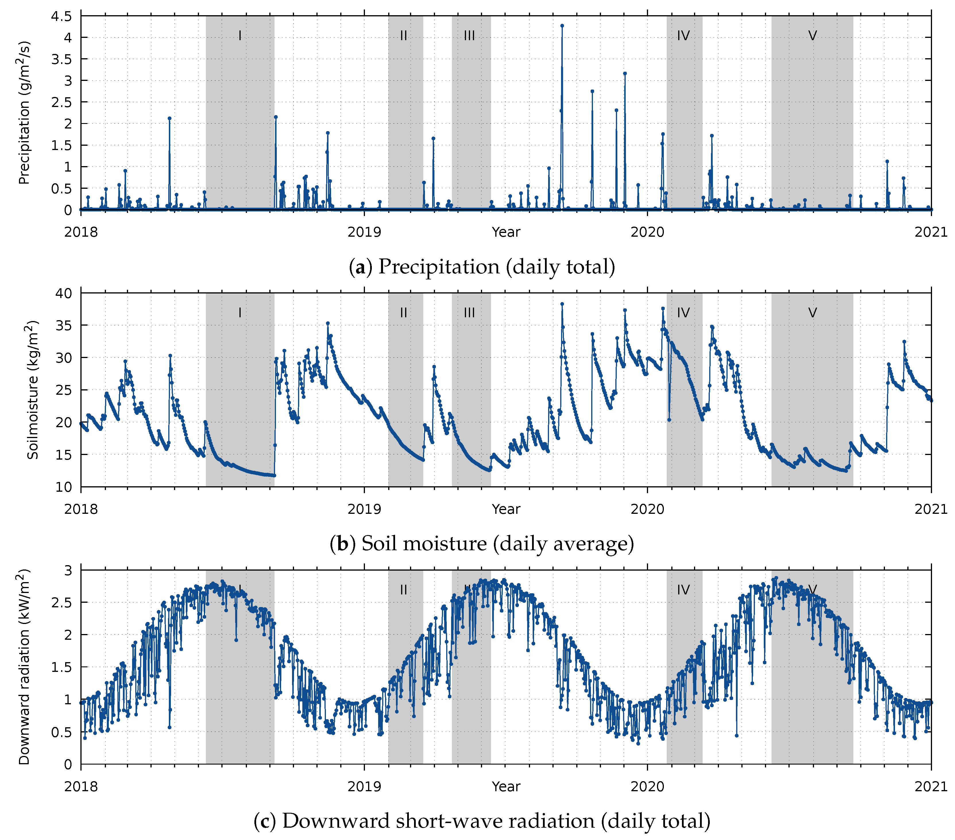
3.1. Observed Weather Conditions

The GLDAS 2.1 meteorological data are shown in Figure 2. From 2018 to 2021, the daily precipitation data (Figure 2a) show rain events that match periods of drying and wetting of the topsoil (Figure 2b). The fluctuations in the downward short-wave radiation data (Figure 2c) correspond with rain events Figure 2a. The fluctuations in the downward short-wave radiation data (Figure 2c) correspond with rainfall events (in Figure 2a). The years 2018 and 2020 both had a single dry period in the summer (period I (June–August) and V (June–September)), after a relatively wet spring (Figure 2a). The year 2019 lacked a relatively long dry period in summer, with two shorter dry periods, in spring (February–March) and in early summer (April–June) (Figure 2a). All three years had a relatively wet autumn (Figure 2b). In all years, the radiation flux was in spring (March–April) generally lower than in the following summer (June–August) (Figure 2c). This implies that elevated soil moisture levels in spring are not only caused by precipitation, but also by less evapotranspiration due to clouds blocking the sun. Following the criteria defined above, there appeared to be five dry periods that show gradual drying of the topsoil (Table 3), with at least 45 days of no or little precipitation. The long periods I and V fall typically in the summer, while periods II and IV fall within early spring and period III in late spring. Periods I–IV have completely no rain, and period V is interrupted by a couple of minor rain events.

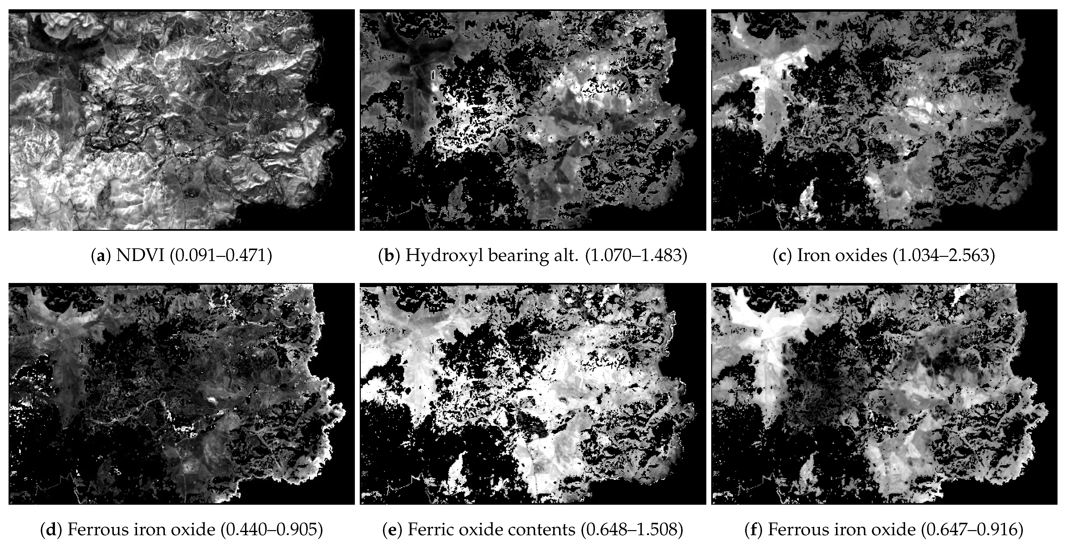
3.2. Image Processing Results

Figure 3 shows the results from applying the vegetation and geological indices to the Sentinel-2 MSI data. The “normalized vegetation difference index” image (Figure 3a) and the location of masked pixels in all images showing a geological index (Figure 3b–e) coincide with green tones of natural vegetation cover in the true-color satellite image (Figure 1b).
The bright pixels in Figure 3b, indicating relatively high values in the “hydroxyl bearing alteration” index, coincide with the expected location of alteration mineralogy and (former) mining locations within the caldera (Figure 1a). The four indices for iron oxides (Figure 3c–f) show patterns that need some interpretation. The pixels with relatively high values for the “iron oxide” index of Sabins [31] (Figure 3c) match with bare soil areas and reddish coloured soils visible in the true-color image (Figure 1b). The indices of Cudahy [10] are designed to differentiate between “ferrous iron oxide” and “ferric iron oxide”. The image results (Figure 3e,f) support this by showing an overall inverse relation between these two indices. There are a few areas that have relatively high index values for both indices. This could physically be explained by the presence of both “ferric iron oxide” and “ferrous iron oxide” spectral signatures in a 20 × 20 m pixel of the Sentinel-2 sensor. As was the case with the “iron oxide” index of Sabins [31] in Figure 3c, the bright pixels of both Cudahy [10] indices fall within areas that can be denoted as bare soil areas and reddish coloured soils in the true-color image (Figure 1b).
The “ferrous iron oxide” of Sabins [31] in Figure 3d should correspond with the “ferrous iron oxide” index of Cudahy [10] in Figure 3f. At a first glance, the results do not seem to match: The highest index values can be found at locations with bare and hard materials, such as rock outcrops, rooftops of buildings, and pebbly beaches. The indices of Cudahy [10] come with a range of index values validated for the ASTER sensor while the indices of Sabins [31] do not come with such a range defined. When ignoring the highest index values and therefore the brightest pixels in the image, it appears that the intermediate (grey) index values do show a spatial pattern in high and low values that matches the index results in Figure 3f. We, therefore, proceed under the assumption that the index results described here can be physically explained and make sense in terms of the application.

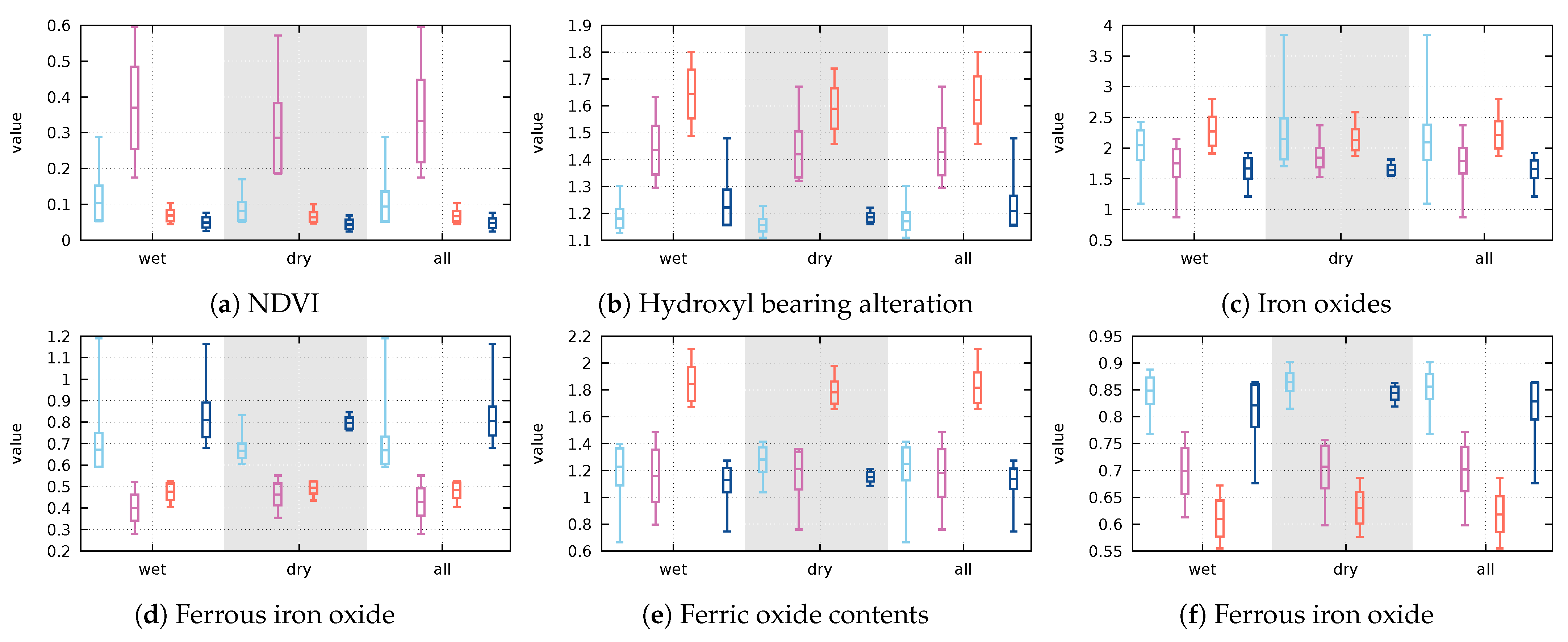
3.3. Indices over Time

Figure 4 shows the variation in index values over the entire three years, in the five dry periods only and the remaining (not dry) periods only. Without exception, the range and standard deviation are relatively smallest in the dry periods (shaded areas in Figure 4). The NDVI (Figure 4a) has a relatively large standard deviation and range in the natural vegetation (), followed by the bare soil area (). The standard deviation in the “hydroxyl bearing alteration” index (Figure 4b) is relatively high in the quarry () and the natural vegetation () and low in the soil () and beach (). However, the range of values is, outside of the dry periods, relatively large in the beach area (). The standard deviation in the “iron oxide” geological indices (Figure 4c–f) seems similar in all areas, although the range can be relatively large in the soil () and the beach () areas, leaving the quarry () as the most stable area over time.

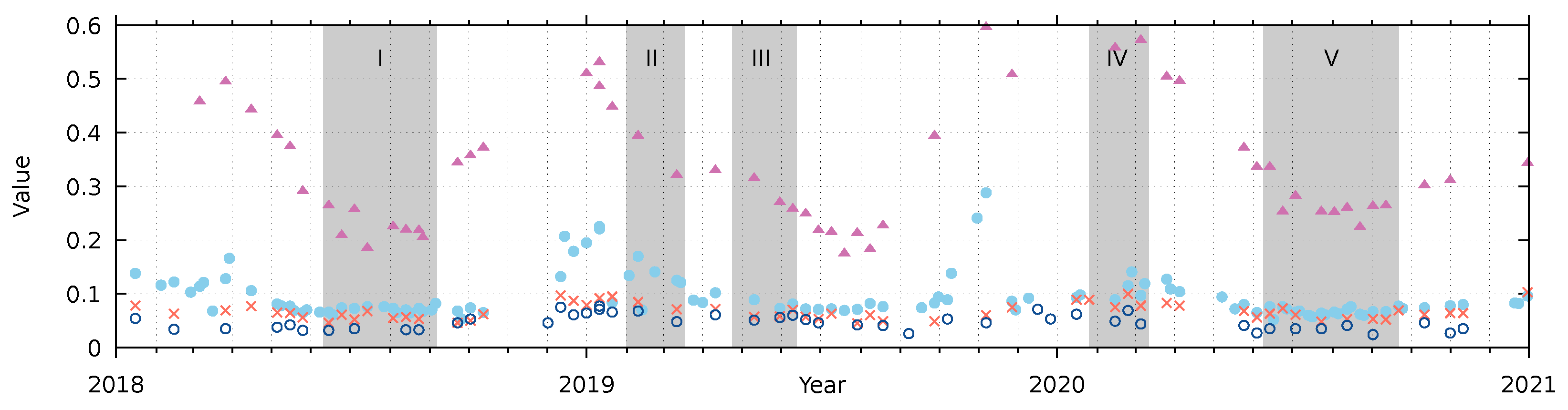
3.4. Vegetation Time Series

Figure 5 shows the temporal behaviour of the NDVI vegetation index. In general, there are more Sentinel-2 MSI data points available in the defined dry periods and summers (Table 3) than in the wet periods. The values originating from the area with natural vegetation () are the highest and show a yearly cycle. Clearly visible are relatively high index values in winter and early spring and relatively low values in summer, the latter coinciding with the dry periods defined in Table 3. Compared to 2018 and 2020, the year 2019 has relatively lower index values in March & April, which coincides with the timespan of the dry period II. The bare soil area () also shows cyclic behaviour that follows the behaviour of natural vegetation, with higher values in autumn, winter and spring. Within the dry periods I, III and V, the index values for the bare soil area seem stable, while in dry periods II and IV they are not. In October 2019, however, there is an abrupt deviation from the index values of the natural vegetation area. The vegetation indices for the quarry (×) and beach () areas are most stable over time, although both areas show slightly higher values in the spring of 2019 and 2020. Looking at the dry periods only, the vegetation indices for all land covers are lowest in periods I and V while slightly elevated in periods II, III and IV. In periods I, IV and V, the beach sand has consistently lower vegetation index values than the quarry, whereas in periods II and III in the year 2019 the values of both landcover types overlap for most of the time.
Looking at the dry periods in Figure 5, the NDVI values follow an annual cycle, with relatively low values in late spring and summer (periods I, III and V) and relatively high values in winter (periods II and IV). Looking within each dry period, the NDVI values appear to be positively correlated with soil moisture; a decrease in soil moisture is accompanied by a decrease in NDVI values, and vice versa. This correlation fits our initial expectations that water availability in the soil leads to the growth of green vegetation in this semi-arid region. From high-resolution satellite images in Table 2 as well as from field visits, it can be observed that the selected natural vegetation area has a permanent presence of vegetation while the quarry might have an occasional shrub. The bare soil and beach sand areas have no expected presence of vegetation. The bare soil area however does show an annual cycle in the vegetation indices, with elevated values in the wet autumn, indicating that some vegetation might be growing in the wet period. In contrast, the few shrubs present in the quarry do not seem to affect the vegetation indices; the level is slightly elevated in autumn, but so is the bare beach sand area.

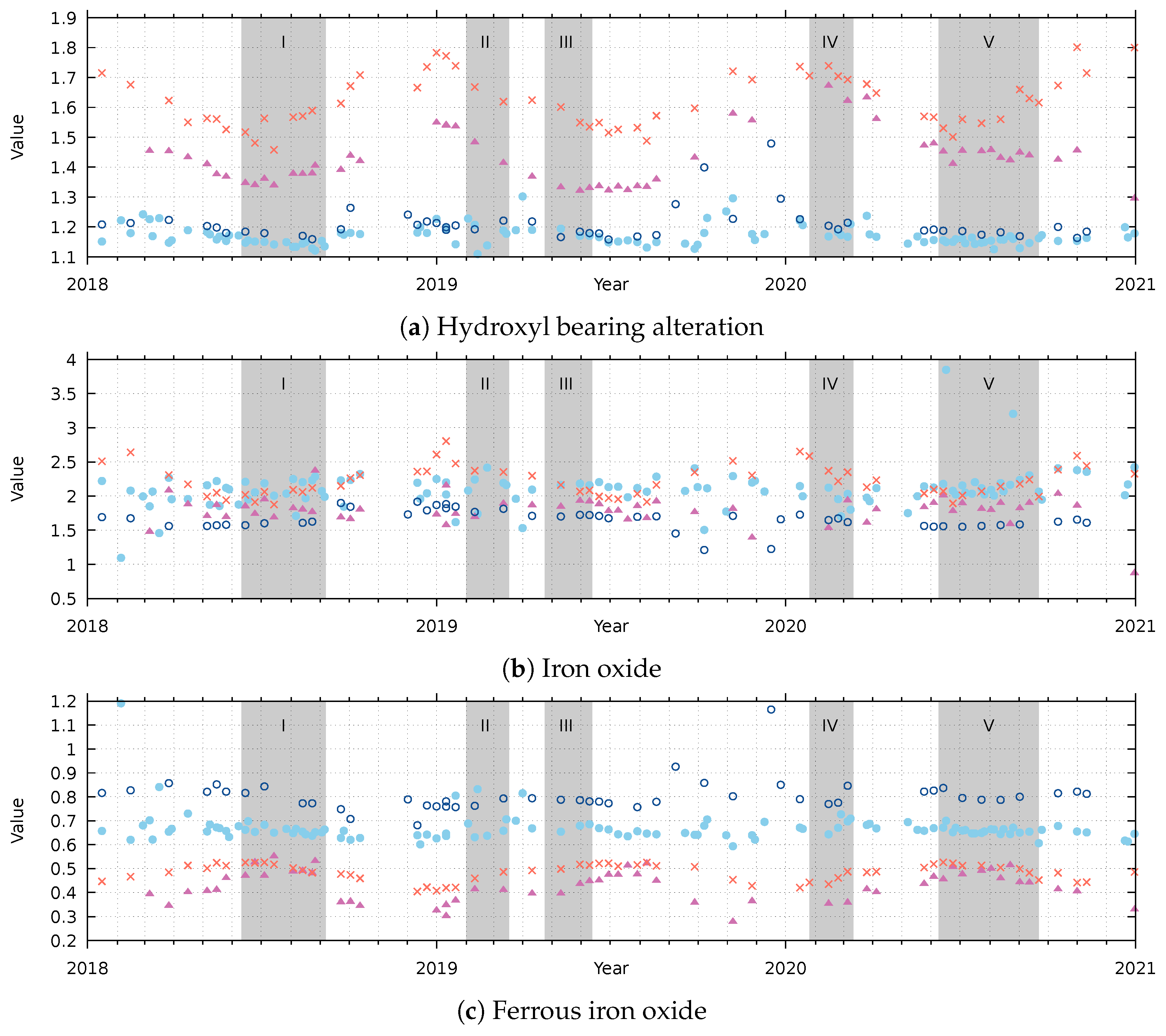
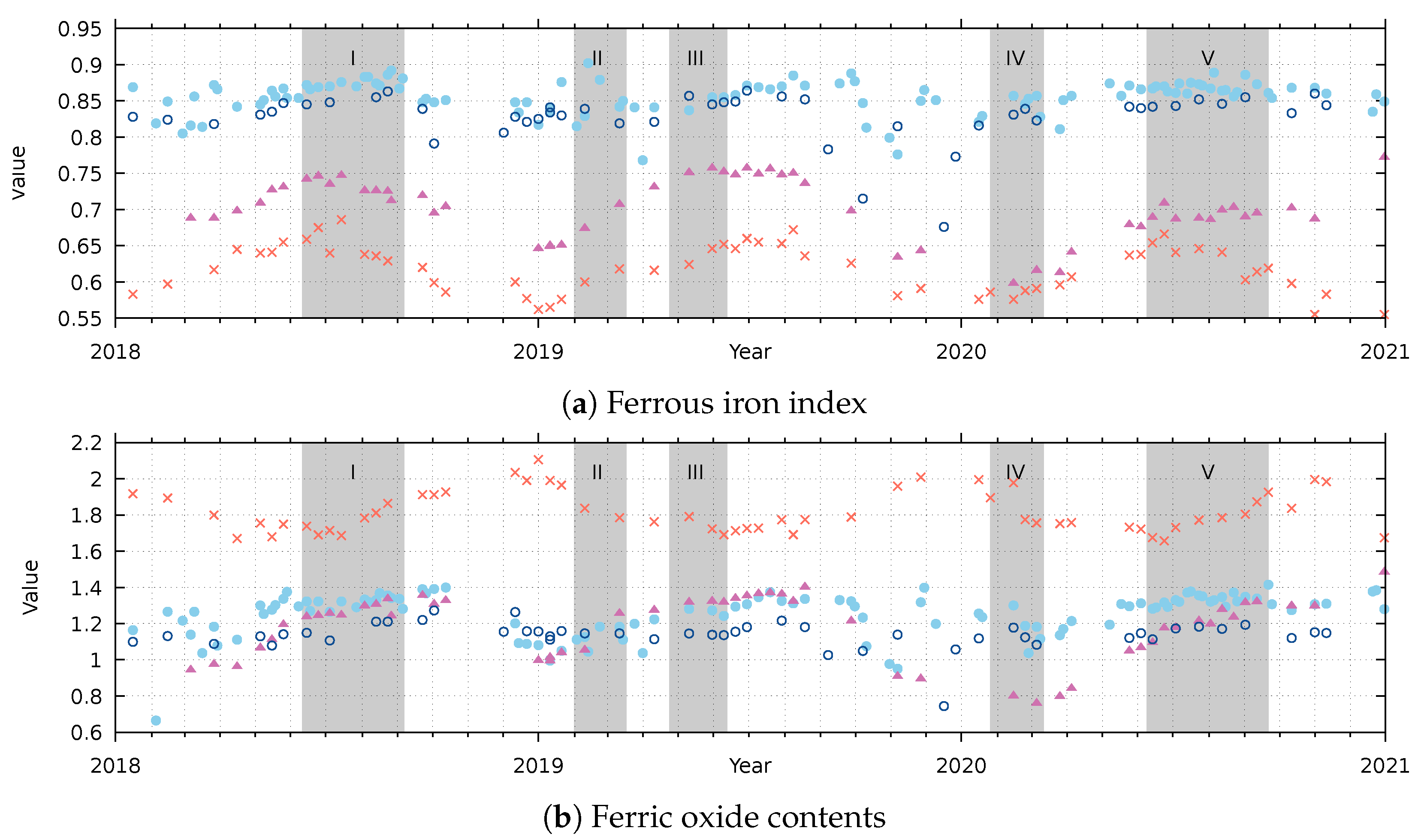
3.5. Geological Time Series

The temporal behaviour of the three geological indices after Sabins [31] is shown in Figure 6. It has to be noted that, due to the cloud masking, fewer data points are available for the beach sand () area. The “hydroxyl bearing alteration” index in Figure 6a clearly shows an effect of seasonality. The values originating from the quarry area (×) are the highest and show an annual cycle, with relatively low/high index values in summer/winter. The values for natural vegetation () are lower than for the quarry but higher than for bare soil and beach sand and also show an annual cycle. The index does not show a cyclic behaviour for the bare soil () and beach sand () areas, although the index values for these areas do vary throughout the year. Outside of the dry periods, large variations for all four areas can be observed, especially during the autumn of 2019. Within the defined dry periods, the “hydroxyl bearing alteration” index values seem most stable over the periods I and V compared to the periods II–IV. While the change in “hydroxyl bearing” index values (Figure 6a) follows the drying of soil (Figure 2b) in dry periods II, III and IV, this relation seems inverted in dry periods I and V. Within the dry periods, small changes in index value seem to correspond with minor rain events (Figure 2a). While the NDVI value of the bare soil area shows a slight change (Figure 5), this surface seems more stable over time than the quarry. This index is, apart from an indicator of mineral alteration, also an indicator for the presence of clay, and a higher index value also indicates that the surface cover might be more susceptible to taking up moisture and thus change the spectral signal. Areas that have a higher index value for “hydroxyl bearing materials” show more signs of annual cyclic behaviour than areas with lower index values.
The “iron oxide” index in Figure 6b shows that observed variation in index values does not allow for easy separation of the four different areas. In general, the highest index values for the quarry (×) and bare soil () areas, and the lowest values for the beach sand () area. The series for the quarry (×) shows a similar annual cyclic behaviour as for the “hydroxyl bearing alteration” index, where this annual cycle is not observable for natural vegetation (). Within the defined periods, the index value for the beach sand () area is very stable, whereas the other areas show some variation. Outside the dry periods, there are times that the index shows large variation, but there are also times that this “iron oxide” index remains stable despite rain events and changing soil moisture (e.g., September–October 2019; June–August 2020; May 2021).
The “ferrous iron oxide” index in Figure 6c shows that, in contrast to the results for the “iron oxide” index, almost consistent separation of index values for each of the four areas is possible. The beach sand () area has the highest index values, with values decreasing for bare soil () and the quarry (×), and lowest index values for the natural vegetation area (). The index shows no annual cyclic behaviour for any of the areas and appears stable most of the time, specifically during the five dry periods. Disturbances are seen during the autumn of 2019 in all four areas, with the highest variation in the natural vegetation () and beach sand () areas.
The temporal behaviour of the three geological indices after Cudahy [10] is shown in Figure 7. The “ferrous iron index” shown in Figure 7a is, after translating the indices from its original definitions to the Sentinel-2 bands as described above in Table 1, the inverse of the “hydroxyl bearing alteration” index of Sabins [31] shown in Figure 6a but allows a direct comparison to the “ferrous iron index” defined by Sabins [31]. This index therefore also shows an effect of seasonality. The values originating from the quarry area (×) are the lowest and show an annual cycle, with relatively high/low index values in summer/winter. The values for natural vegetation () are higher than for the quarry but lower than for bare soil and beach sand and also show an annual cycle. The index does not show a cyclic behaviour in the bare soil () and beach sand () areas, although the index values for these areas do vary throughout the year. Outside of the dry periods, large variations for all four areas can be observed, especially during the autumn of 2019. Within the defined dry periods, the “ferrous iron index” index values seem most stable over the periods I and V compared to the periods II–IV.
The values of the “ferric oxide contents“ index in Figure 7b are highest for the quarry (×). In temporal behaviour, it can be observed that the index values for the quarry (×) area increase over autumn and winter, whereas, for the other three areas, the index values decline. The values for the other three areas are relatively close to each other, where the values for bare soil () are, overall, slightly higher than for beach sand (). The values for natural vegetation () show the largest annual cycle, being sometimes the lowest and sometimes the highest of these three. Within the defined longer dry periods I and V, this index shows an increase over time, which is in line with the observed decline in soil moisture (Figure 2b). For the shorter dry periods II, III and IV, the index seems stable but not for all data points. The index values for natural vegetation () show an annual cyclic behaviour with minimum values during winter, whereas for the other areas the index values are less season-dependent. Within all dry periods, the index value for beach sand () is the lowest and appears as being the most stable. However, for all other geological indices, the long dry periods I and V appear to behave very similarly, the natural vegetation (), quarry (×) and bare soil () show large variation in “ferric oxide composition“ index during period I and a more stable behaviour for period V.

4. Discussion

The aim of this study is to test the repeatability of spectral indices to allow for continental-scale mineral mapping using multiple stacked and mosaicked images. We therefore evaluate the influence of precipitation and soil moisture conditions on the variance of several “geological” spectral indices over time.
The meteorological data in Figure 2 show that 2018 and 2020 had similar weather patterns throughout the year, with a relatively wet spring, a dry summer with a relatively long dry period, and a wet autumn. The year 2019 is an exceptional year, with two shorter dry periods in spring and a relatively wet summer, and no dry periods longer than 50 days. The definition of the five dry periods is arbitrarily set to approx. 45 days without rain, which left some differences between these periods. Of the 5 dry periods that we defined, periods I and V are the longest and also have the lowest soil moisture level (Table 3. Periods II–IV are considerably shorter. While periods II and III have still relatively low soil moisture, period IV did not reach a soil moisture level below 15 kg/m 2 like the other periods. The few (minor) rain events that occurred during period V, which had relatively low soil moisture, did not really influence the spectral index values.
For geological remote sensing, an unobstructed view of rocks and soil is required for optimal conditions. Pixels affected by a vegetation cover should therefore be masked, for example by thresholding an NDVI image, or by using a multi-temporal dataset to select the barest pixels over time, following Roberts et al. [12]. Figure 5 shows that all pixels with an NDVI value above 0.1 ought to be masked to avoid any influence of vegetation. This is considerably more conservative than the threshold of 0.4 used by e.g., Hewson et al. [40]. Our threshold is also lower than the threshold used by Cudahy [10], which has a valid range of 1.4–4.0 for a simple NIR/Red band ratio to label vegetation presence from relatively low to relatively high: Converting our NDVI threshold of 0.1 to the band ratio of Cudahy [10] leaves a threshold of 1.2 as the separation criterion, which is below the published lower limit for this ratio. Despite setting this low threshold for masking pixels with vegetation, the NDVI values of the bare soil polygon still show differences between the wet and dry periods. In contrast, the NDVI values for the quarry and beach sand polygons do not change. This suggests that using geological remote sensing results on soils can hardly be compared over time unless the soil is as bare as a beach or the rocky floor of a quarry.
Logically, temporal variation in spectral indices occurs in areas with vegetation presence, as well as in a period of time when there is frequent rain (Figure 5, Figure 6 and Figure 7). However, even when focusing solely on the dry periods in spring and summer, variation can still be observed even in the selected, relatively pure, areas where one would expect little change over time (Figure 4). Table 2 shows that the quarry might have sparse vegetation present and Figure 6 and Figure 7 show that bare soil areas might still have vegetation growth over time. The beach area seems stable but can suffer from water coming out of a stream, leaving a moist patch of sand that could influence the mineral spectral indices.
Apart from such physical changes at the earth’s surface, another factor that is not addressed in this research is the effect of atmospheric correction. The spectral indices used in this paper are based on Sentinel-2 MSI bands 2, 3, 4, 8, 11 and 12 (Table 1), covering a 0.49–2.19 μm wavelength range. Depending on the wavelengths covered, bands could be affected by scattering of light and atmospheric absorption. Bands 2 and 3 are affected by scattering of light in the atmosphere, and pixel values of these bands depend more on the quality of the atmospheric correction than other bands. Other wavelengths could be affected by choices made in model-based atmospheric correction. Figure 2 in Hewson et al. [41] shows, for example, the effect of choosing different standard atmospheric composition on the correction of ASTER data. Consequently, any of the band ratios used in this paper, but especially the “iron oxide” index of Sabins [31] because of using band 2, could reflect the effect of measuring at different times of the year and with different atmospheric conditions. However, when mapping on a continental or global scale, it is not feasible to do tailor-made adjustments to the atmospheric correction. Therefore, we decided to take the data and methods “as is” and only used data selection as a means to come to data collection.
For the same reason, this study also does not go into detail to understand the observed changes in spectral indices. Instead, we leave it to the practical conclusion that the level of soil moisture and change in soil moisture is equally important, if not more important than the amount of rain that falls. A multi-temporal approach helps to come to a better selection of data, for continental-scale mapping where multi-temporal data are used as well as for studies that could be carried out on a single image only.
For testing the repeatability of spectral indices used in geological remote sensing, Sentinel-2 MSI is an excellent choice. The 6-day return time of the Sentinel-2 constellation creates a sufficiently large data volume to perform this experiment, even when limiting the data selection to only one of the two available sensors and one specific orbit. Some of the dry periods still have rather few data points due to cloud masking; however, it is sufficient to observe the behaviour of spectral indices in terms of variance over time. Including data from Sentinel-2B as well as involving data acquired in different orbits would have increased data points but also increased noise in our results due to calibration differences (not shown). We chose to ignore these additional sources of noise, as we strive to discuss the principle of weather (availability of atmospheric and soil moisture) influencing the repeatability of geological remote sensing in a semi-arid region.
The creation of seamless cross-continental geoscience products has been described extensively by Caccetta et al. [42] and, for a smaller area, by Hewson et al. [41]. Image selection from the 8 years of ASTER data underlying these mosaics was achieved by the criteria ‘cloud free, high sun angle summer scenes which minimized the presence of vegetation” [42], while extensive calibration between scenes and user interventions were needed to come to seamless mosaics. Figure 2 in Caccetta et al. [42] shows that some areas were covered by single ASTER scenes, meaning that data selection possibilities were eventually limited. The 2019 mosaic published by Roberts et al. [12] could select from 30 years of Landsat data, while the Sentinel-2 based mosaic published by Wilford and Roberts [19] makes use of the vast Sentinel-2 archive build up since 2015. Present-day computing power allows for selecting optimal pixels instead of optimal scenes but requires data from continuous operational missions such as Landsat and Sentinel to reach an optimal moment of acquisition and selection of data. The focus in creating the latter mosaics seems, however, to have been on masking vegetation and clouds to obtain an unobstructed view. Our results show that further optimization of this selection process should, in order to come to more repeatable measurements, include weather parameters. Ideally, it should result in a product that is repeatable at other moments, as well as applicable to an area covered with multiple scenes.
Selecting this moment is also important even when only a single remote sensing image would be needed, and should be based on a multi-temporal analysis: typically, remote sensing geologists would select an image in summer, preferably a few days after the last rainfall. Our results show that spectral indices are still affected after these few days of no rain, even when measured on bare soil and rock surfaces within dry periods of the year. The classic approach of selecting an image by visual inspection and cloud cover statistics does not necessarily result in the best choice of data. The relation between soil moisture and index values in the five dry periods indicates that the effect of precipitation, via soil moisture, does not disappear in a few days. In addition, the soil moisture change is not the same in every year. Based on these observations, it appears that, for a mineral spectral index to be least variant over time, and provided an unobstructed view and adequate atmospheric correction that a low soil moisture level is needed in the first place, and that minor (rain) events do not have much of an effect on results.

5. Conclusions

Geological remote sensing often does not involve a factor time, given that information sought changes in geological time and not in human time. The weather and seasonal changes, however, do affect the conditions in which measurements are taken. By looking at the temporal behaviour of several spectral indices in 3 year Sentinel-2 MSI data, several “rules of thumb” used in geological remote sensing could be confirmed. At the same time, some could be sharpened or even need to be changed. Even in remote sensing studies where the factor time does not play a role, a multi-temporal approach is still justified to come to an optimal data selection, especially for areas with precipitation.
Even when taking an atmospheric correction and unexpected ground cover change for granted and not going into detailed analysis for correcting factors, meaning that there might be lasting limitations for reliable large scale regional to continental quantifiable mineral index mapping, a multi-temporal approach allows for a more critical and improved data selection.
Spectral indices for geological remote sensing have the best chance of being invariant in the (local) summer, not only because the sun is then the highest in the sky but also because the surface is likely at its driest. An overall low soil-moisture level appears to be more important for the repeatability of spectral index values over time than the avoidance of minor rain events. Although there is no generic approach for masking vegetation in geological remote sensing, it appears that, for this semi-arid area and for data acquired at any time of the year, NDVI thresholds for masking should not be higher than 0.1. Selection of data should therefore not be based only on a certain number of days without rain in the days preceding data acquisition, or the lowest vegetation cover possible, but also include soil moisture conditions. While the results for the years 2018 and 2020 illustrate these statements, the result for the year 2019, indicating abnormal weather conditions, state that this finding does not have to apply each year. Consequently, weather data should be incorporated in coming to an optimal selection of remote sensing imagery, and also be used when analyzing multi-temporal data.
The influence of the solar zenith and azimuth is not easy to determine in this dataset, as the winter months coincide with less data availability, more rain events, higher soil moisture levels and a more dense vegetation cover. Repeating this study in a different climate zone, where changes in illumination coincide with less changes of other environmental variables, is therefore a possible follow up study.
Similarly, the influence of the atmospheric correction is not easy to determine in these data. It would be possible to extend this study with observations on temporal behaviour of bands used for atmospheric parameters, e.g., Sentinel-2 MSI band 10, and atmospheric parameters obtained in the atmospheric correction (e.g., water vapor estimates). Lastly, future studies could include field soil moisture measurements to quantify the role soil moisture and possibly come to corrections rather than only observations. A numerical relation between atmospheric and ground affected moisture with spectral indices, and possibly also other environmental parameters that did not appear as influential as ground moisture in our experiment, should be tested in a study covering a larger area, to reach a generic conclusion.

Author Contributions

Conceptualization, H.v.d.W., J.E. and R.H.; methodology, H.v.d.W., A.S. and J.E.; software, H.v.d.W. and A.S.; writing—original draft preparation, H.v.d.W.; writing—review and editing, J.E., A.S. and R.H.; visualization, H.v.d.W. and J.E. All authors have read and agreed to the published version of the manuscript.

Funding

This research received no external funding.

Data Availability Statement

The Sentinel-2 MSI level 2A image data, and GLDAS 2.1 and ERA5 meteorological data, supporting this manuscript can be accessed free of charge following the cited references or via the Google Earth Engine. ERA5 data Hersbach et al. [29] is provided by the Copernicus Climate Change Service (C3S) Climate Data Store; the results contain modified Copernicus Climate Change Service information 2020. Neither the European Commission nor ECMWF is responsible for any use that may be made of the Copernicus information or data it contains.

Conflicts of Interest

The authors declare no conflict of interest.

Abbreviations

The following abbreviations are used in this manuscript:
ASTERAdvanced Spaceborne Thermal Emission and Reflection Radiometer
ESAEuropean Space Agency
GEEGoogle Earth Engine
GLDASGlobal Land Data Assimilation System
MSIMultiSpectral Instrument
MSSMultiSpectral Scanner
NDVINormalized Difference Vegetation Index
NIRNear InfraRed
SCLScene Classification Layer
SWIRShortWave InfraRed
TMThematic Mapper
VNIRVisible & Near InfraRed

References

  1. Cooper, B.L.; Salisbury, J.W.; Killen, R.M.; Potter, A.E. Midinfrared spectral features of rocks and their powders. J. Geophys. Res.-Planets 2002, 107. [Google Scholar] [CrossRef]
  2. Salisbury, J.W.; Walter, L.S.; Vergo, N. Availability of a library of infrared (2.1–25.0 μm) mineral spectra. Am. Mineral. 1989, 74, 938–939. [Google Scholar]
  3. Hunt, G. Spectral signatures of particulate minerals in the visible and near-infrared. Geophysics 1977, 42, 501–513. [Google Scholar] [CrossRef] [Green Version]
  4. Goetz, A.; Rowan, L. Geologic remote-sensing. Science 1981, 211, 781–791. [Google Scholar] [CrossRef]
  5. Crósta, A.; Moore, J. Geological mapping using Landsat Thematic Mapper imagery in Almeria Province, south-east Spain. Int. J. Remote Sens. 1989, 10, 505–512. [Google Scholar] [CrossRef]
  6. Abrams, M. The Advanced Spaceborne Thermal Emission and Reflection Radiometer (ASTER): Data products for the high spatial resolution imager on NASA’s Terra platform. Int. J. Remote Sens. 2000, 21, 847–859. [Google Scholar] [CrossRef]
  7. Yamaguchi, Y.; Kahle, A.B.; Tsu, H.; Kawakami, T.; Pniel, M. Overview of Advanced Spaceborne Thermal Emission and Reflection Radiometer (ASTER). IEEE Trans. Geosci. Remote Sens. 1998, 36, 1062–1071. [Google Scholar] [CrossRef] [Green Version]
  8. Abrams, M.; Hook, S.J. Simulated ASTER data for geologic studies. IEEE Trans. Geosci. Remote Sens. 1995, 33, 692–699. [Google Scholar] [CrossRef]
  9. Hewson, R.; Robson, D.; Mauger, A.; Cudahy, T.; Thomas, M.; Jones, S. Using the Geoscience Australia-CSIRO ASTER maps and airborne geophysics to explore Australian geoscience. J. Spat. Sci. 2015, 60, 207–231. [Google Scholar] [CrossRef]
  10. Cudahy, T. Australian ASTER Geoscience Product Notes; Technical Report; Commonwealth Scientific and Industrial Research Organisation (CSIRO): Canberra, Australia, 2012. [Google Scholar] [CrossRef]
  11. Wilford, J.; Roberts, D. Enhanced Bare Earth Covariates for Soil and Lithological Modelling. Version 1.0. Terrestrial Ecosystem Research Network. Dataset. 2021. Available online: https://portal.tern.org.au/enhanced-bare-earth-lithological-modelling/21910 (accessed on 18 November 2022).
  12. Roberts, D.; Wilford, J.; Ghattas, O. Exposed soil and mineral map of the Australian continent revealing the land at its barest. Nat. Commun. 2019, 10, 11. [Google Scholar] [CrossRef]
  13. Hewson, R.; van der Werff, H.; Hecker, C.; van Ruitenbeek, F.; Bakker, W.; van der Meijde, M. Status and Developments in Geological Remote Sensing. FastTIMES 2020, 25, 54–66. [Google Scholar]
  14. Soydan, H.; Koz, A.; Şebnem Düzgün, H. Secondary Iron Mineral Detection via Hyperspectral Unmixing Analysis with Sentinel-2 Imagery. Int. J. Appl. Earth Obs. Geoinf. 2021, 101, 102343. [Google Scholar] [CrossRef]
  15. van der Werff, H.; van der Meer, F. Sentinel-2A MSI and Landsat 8 OLI Provide Data Continuity for Geological Remote Sensing. Remote Sens. 2016, 8, 883. [Google Scholar] [CrossRef] [Green Version]
  16. van der Werff, H.; van der Meer, F. Sentinel-2 for mapping iron absorption feature parameters. Remote Sens. 2015, 7, 12635–12653. [Google Scholar] [CrossRef] [Green Version]
  17. van der Meer, F.; van der Werff, H.; van Ruitenbeek, F. Potential of ESA’s Sentinel-2 for geological applications. Remote Sens. Environ. 2014, 148, 124–133. [Google Scholar] [CrossRef]
  18. Mielke, C.; Boesche, N.; Rogass, C.; Kaufmann, H.; Gauert, C.; de Wit, M. Spaceborne Mine Waste Mineralogy Monitoring in South Africa, Applications for Modern Push-Broom Missions: Hyperion/OLI and EnMAP/Sentinel-2. Remote Sens. 2014, 6, 6790–6816. [Google Scholar] [CrossRef] [Green Version]
  19. Wilford, J.; Roberts, D. Sentinel-2 Barest Earth Imagery for Soil and Lithological Mapping; Geoscience: Canberra, Australia, 2021. [Google Scholar] [CrossRef]
  20. Rowan, L.C.; Mars, J.C. Lithologic mapping in the Mountain Pass, California area using Advanced Spaceborne Thermal Emission and Reflection Radiometer (ASTER) data. Remote Sens. Environ. 2003, 84, 350–366. [Google Scholar] [CrossRef]
  21. Cudahy, T.; Caccetta, M.; Thomas, M.; Hewson, R.; Abrams, M.; Kato, M.; Kashimura, O.; Ninomiya, Y.; Yamaguchi, Y.; Collings, S.; et al. Satellite-derived mineral mapping and monitoring of weathering, deposition and erosion. Sci. Rep. 2016, 6, 23702. [Google Scholar] [CrossRef] [Green Version]
  22. van der Meer, F.; van der Werff, H.; van Ruitenbeek, F.; Hecker, C.; Bakker, W.; Noomen, M.; van der Meijde, M.; Carranza, E.; de Smeth, J.; Woldai, T. Multi- and hyperspectral geologic remote sensing: A review. Int. J. Appl. Earth Obs. Geoinf. 2012, 14, 112–128. [Google Scholar] [CrossRef]
  23. van der Werff, H.; Hewson, R.; van der Meer, F. Use What Is There: What Can Sentinel-2 Do for Geological Remote Sensing? In Proceedings of the IGARSS 2018—2018 IEEE International Geoscience and Remote Sensing Symposium, Valencia, Spain, 22–27 July 2018; IEEE: Valencia, Spain, 2018. [Google Scholar] [CrossRef]
  24. Langford, R.L. Temporal merging of remote sensing data to enhance spectral regolith, lithological and alteration patterns for regional mineral exploration. Ore Geol. Rev. 2015, 68, 14–29. [Google Scholar] [CrossRef]
  25. Gorelick, N.; Hancher, M.; Dixon, M.; Ilyushchenko, S.; Thau, D.; Moore, R. Google Earth Engine: Planetary-scale geospatial analysis for everyone. Remote Sens. Environ. 2017, 202, 18–27. [Google Scholar] [CrossRef]
  26. Beaudoing, H.; Rodell, M. GLDAS Noah Land Surface Model L4 3 Hourly 0.25 × 0.25 Degree V2.1. 2020. Available online: https://disc.gsfc.nasa.gov/datasets/GLDAS_NOAH025_3H_2.1/summary (accessed on 18 November 2022).
  27. Rodell, M.; Houser, P.; Jambor, U.; Gottschalck, J.; Mitchell, K.; Meng, C.; Arsenault, K.; Cosgrove, B.; Radakovich, J.; Bosilovich, M.; et al. The Global Land Data Assimilation System. Bull. Amer. Meteor. Soc. 2004, 85, 381–394. [Google Scholar] [CrossRef] [Green Version]
  28. Muñoz Sabater, J. ERA5-Land Hourly Data from 1981 to Present. Copernicus Climate Change Service (C3S) Climate Data Store (CDS). 2019. Available online: https://cds.climate.copernicus.eu/cdsapp#!/dataset/10.24381/cds.e2161bac?tab=overview (accessed on 18 November 2022).
  29. Hersbach, H.; Bell, B.; Berrisford, P.; Biavati, G.; Horányi, A.; Muñoz Sabater, J.; Nicolas, J.; Peubey, C.; Radu, R.; Rozum, I.; et al. ERA5 Hourly Data on Single Levels from 1979 to Present. Copernicus Climate Change Service (C3S) Climate Data Store (CDS). 2018. Available online: https://cds.climate.copernicus.eu/cdsapp#!/dataset/reanalysis-era5-single-levels?tab=overview (accessed on 18 November 2022).
  30. Berger, M.; Moreno, J.; Johannessen, J.A.; Levelt, P.F.; Hanssen, R.F. ESA’s sentinel missions in support of Earth system science. Remote Sens. Environ. 2012, 120, 84–90. [Google Scholar] [CrossRef]
  31. Sabins, F.F. Remote sensing for mineral exploration. Ore Geol. Rev. 1999, 14, 157–183. [Google Scholar] [CrossRef]
  32. Drusch, M.; Del Bello, U.; Carlier, S.; Colin, O.; Fernandez, V.; Gascon, F.; Hoersch, B.; Isola, C.; Laberinti, P.; Martimort, P.; et al. Sentinel-2: ESA’s Optical High-Resolution Mission for GMES Operational Services. Remote Sens. Environ. 2012, 120, 25–36. [Google Scholar] [CrossRef]
  33. Huete, A. A Soil-Adjusted Vegetation Index (SAVI). Remote Sens. Environ. 1988, 25, 295–309. [Google Scholar] [CrossRef]
  34. ESA. Sentinel-2 L1C Data Quality Report. 2022. Available online: https://sentinel.esa.int/documents/247904/685211/Sentinel-2_L1C_Data_Quality_Report (accessed on 18 November 2022).
  35. ESA. Sentinel-2 MSI Level-2A Algorithm Overview. Available online: https://sentinel.esa.int/web/sentinel/technical-guides/sentinel-2-msi/level-2a/algorithm (accessed on 18 November 2022).
  36. Bhatia, N.; Iordache, M.D.; Stein, A.; Reusen, I.; Tolpekin, V. Propagation of uncertainty in atmospheric parameters to hyperspectral unmixing. Remote Sens. Environ. 2018, 204, 472–484. [Google Scholar] [CrossRef]
  37. Schäpfer, D.; Borel, C.; Keller, J.; Itten, K. Atmospheric precorrected differential absorption technique to retrieve columnar water vapor. Remote Sens. Environ. 1998, 65, 353–366. [Google Scholar] [CrossRef]
  38. ESA. Level-2A Prototype Processor for Atmospheric, Terrain and Cirrus Correction of Top-Of-Atmosphere Level 1C Input Data. Available online: http://step.esa.int/main/third-party-plugins-2/sen2cor/ (accessed on 18 November 2022).
  39. Arribas, A.; Cunningham, C.; Rytuba, J.; Rye, R.; Kelly, W.; Podwysocki, M.; McKee, E.; Tosdal, R. Geology, geochronology, fluid inclusions, and isotope geochemistry of the Rodalquilar gold alunite deposit, Spain. Econ. Geol. 1995, 90, 795–822. [Google Scholar] [CrossRef]
  40. Hewson, R.; Mshiu, E.; Hecker, C.; van der Werff, H.; van Ruitenbeek, F.; Alkema, D.; van der Meer, F. The application of day and night time ASTER satellite imagery for geothermal and mineral mapping in East Africa. Int. J. Appl. Earth Obs. Geoinf. 2020, 85, 13. [Google Scholar] [CrossRef]
  41. Hewson, R.; Cudahy, T.; Mizuhiko, S.; Ueda, K.; Mauger, A. Seamless geological map generation using ASTER in the Broken Hill—Curnamona province of Australia. Remote Sens. Environ. 2005, 99, 159–172. [Google Scholar] [CrossRef]
  42. Caccetta, M.; Collings, S.; Cudahy, T. A calibration methodology for continental scale mapping using ASTER imagery. Remote Sens. Environ. 2013, 139, 306–317. [Google Scholar] [CrossRef]
Figure 1. (a) shows the location of the Cabo de Gata area in Spain and the spatial extent of the images used in this research (indicated by the red box). These data overlie a geological map modified after Arribas et al. [39] showing lithologic units around the town of Rodalquilar. (b) shows a Worldview-3 true colour composite (R: 660 nm, G: 547 nm, B: 482 nm) acquired on 13 September 2017 with natural vegetation in greenish tones, bare soil and rock in white & reddish tones, and water bodies and the Mediterranean sea in dark tones.
Remotesensing 14 06303 g001aRemotesensing 14 06303 g001b
Figure 2. Meteorological parameters (a) daily total precipitation; (b) daily average soil moisture (0–10 cm depth) and (c) average downward SWIR radiation flux [26,27]. Five dry periods longer than 45 days (Table 3) are indicated by a grey-shaded background.
Remotesensing 14 06303 g002
Figure 3. Sentinel-2 MSI images showing the mean index values of a 3-year timespan: (a) NDVI and geological indices after (bd) Sabins [31] and (e,f) Cudahy [10]. Pixels with negative NDVI value, indicative of water, are masked in all images. The geological indices are also masked for vegetation by allowing only pixels with an NDVI value of 0.15 or lower. The images are shown in a 98% linear stretch, with value ranges mentioned in the subcaption.
Remotesensing 14 06303 g003
Figure 4. Summary statistics of soil moisture on the values of six spectral indices: (a) NDVI, (bd) three geological band ratios after Sabins [31] and (e,f) two geological band ratios after Cudahy [10]. The colors indicate the surface cover: bare soil, natural vegetation, quarry, and beach sand.
Remotesensing 14 06303 g004
Figure 5. NDVI time series for () natural vegetation, () bare soil, (×) quarry floor and () beach sand pixels. The five dry periods longer than 45 days (Table 3) are indicated by a grey-shaded background.
Remotesensing 14 06303 g005
Figure 6. Time series of geological indices (a) Hydroxyl bearing alteration; (b) Iron oxide and (c) Ferrous iron oxide, after Sabins [31]. The data are for () natural vegetation; () bare soil; (×) quarry; and () beach sand. The five dry periods longer than 45 days (Table 3) are indicated by a grey-shaded background.
Remotesensing 14 06303 g006
Figure 7. Time series of geological indices (a) Ferrous iron index and (b) Ferric oxide contents, after Cudahy [10]. The data are for () natural vegetation; () bare soil; (×) quarry; and () beach sand. The five dry periods longer than 45 days (Table 3) are indicated by a grey-shaded background.
Remotesensing 14 06303 g007
Table 1. Sentinel-2 MSI spectral indices used in this paper. The Sentinel-2 MSI indices bands are created after indices originally developed for Landsat TM [31] and ASTER [10] as proxies for mapping mineralogy, using bands equivalent to the ASTER and LANDSAT TM bands. A comparison of these indices between Sentinel-2, Landsat TM and ASTER bands can be found in van der Werff and van der Meer [15].
FeatureSourceASTERLandsat TMSentinel-2
NDVIHuete [33](3−2)/(3+2)(4−3)/(4+3)(8−4)/(8+4)
Hydroxyl bearing alterationSabins [31] 5/711/12
All iron oxides 3/14/2
Ferrous iron oxides 3/54/11
Ferric oxide contents, Fe 3 + Cudahy [10]4/3 11/8
Ferric oxide composition, Fe 3 + 2/1 4/3
Ferrous iron index, Fe 2 + 5/4 12/11
Table 2. The four regions of interest in the Rodalquilar area and their characteristics. The images consist of a high-spatial-resolution Google Earth backdrop (Dated 16 July 2018) overlaid with a semi-transparent NDVI image created with 20 m. pixels of the Sentinel-2 MSI sensor. The 10 × 10 and 20 × 20 m. polygons sampled are shown as red boxes in each image. The polygons do not appear as an exact square as these were defined in the EPSG:3857 geographic coordinate system used in the Google Earth Engine. The geographic coordinates indicate the centre of each polygon.
Remotesensing 14 06303 i001Bare soilRemotesensing 14 06303 i002Beach sand
2.07455E, 36.86685N2.00555E, 36.85900N
10 × 10 m. dirt road crossing, disturbed by infrequent traffic and therefore mostly kept bare.10 × 10 m. beach at a stream mouth, therefore occasionally wet and possibly disturbed by sunbathers.
Remotesensing 14 06303 i003Quarry floorRemotesensing 14 06303 i004Natural vegetation
2.06125E, 36.85800N2.06239E, 36.86840N
10 × 10 m. mix of rock, dirt and an occasional shrub. Unlikely to be disturbed over time but there may be shadows.20 × 20 m. mix of vegetation and natural soil. Unlikely to be disturbed over time but shows seasonal change.
Table 3. Definition of the five selected dry periods, with at least 45 days of no or little precipitation, in the years 2018–2021.
PeriodFromToLength (days)# Images
I11 Jun 20187 Sep 2018888
II1 Feb 201918 Mar 2019455
III24 Apr 201913 Jun 2019505
IV26 Jan 202012 Mar 2020465
V9 Jun 202022 Sep 202010511
Publisher’s Note: MDPI stays neutral with regard to jurisdictional claims in published maps and institutional affiliations.

