Article

Unsupervised Adversarial Domain Adaptation for Agricultural Land Extraction of Remote Sensing Images

1
College of Information Engineering, Sichuan Agricultural University, Ya’an 625000, China
2
College of Resources, Sichuan Agricultural University, Chengdu 611130, China
*
Author to whom correspondence should be addressed.
These authors contributed equally to this work.
Remote Sens. 2022, 14(24), 6298; https://doi.org/10.3390/rs14246298
Submission received: 6 November 2022 / Revised: 6 December 2022 / Accepted: 9 December 2022 / Published: 12 December 2022

Abstract

:
Agricultural land extraction is an essential technical means to promote sustainable agricultural development and modernization research. Existing supervised algorithms rely on many finely annotated remote-sensing images, which is both time-consuming and expensive. One way to reduce the annotation cost approach is to migrate models trained on existing annotated data (source domain) to unannotated data (target domain). However, model generalization capability is often unsatisfactory due to the limit of the domain gap. In this work, we use an unsupervised adversarial domain adaptation method to train a neural network to close the gap between the source and target domains for unsupervised agricultural land extraction. The overall approach consists of two phases: inter-domain and intra-domain adaptation. In the inter-domain adaptation, we use a generative adversarial network (GAN) to reduce the inter-domain gap between the source domain (labeled dataset) and the target domain (unlabeled dataset). The transformer with robust long-range dependency modeling acts as the backbone of the generator. In addition, the multi-scale feature fusion (MSFF) module is designed in the generator to accommodate remote sensing datasets with different spatial resolutions. Further, we use an entropy-based approach to divide the target domain. The target domain is divided into two subdomains, easy split images and hard split images. By training against each other between the two subdomains, we reduce the intra-domain gap. Experiments results on the “DeepGlobe → LoveDA”, “GID → LoveDA” and “DeepGlobe → GID” unsupervised agricultural land extraction tasks demonstrate the effectiveness of our method and its superiority to other unsupervised domain adaptation techniques.

Graphical Abstract

1. Introduction

Agricultural land is an essential resource for human survival, which can provide us with the raw materials necessary for production and life [1]. The automatic segmentation of agricultural land is an essential technical means to promote sustainable agricultural development and modernization research [2]. Remote sensing images are used for agricultural land monitoring under their high timeliness and wide coverage [3,4,5,6]. Agricultural land extraction aims to extract the agricultural land pixels from remote sensing images. The images generated by the different sensors vary considerably. There are also significant differences in the distribution of agricultural land in different regions or the same region at different times. In addition, there are significant challenges in the data annotation of remote-sensing images. As a result, identifying agricultural land in remote-sensing images is a difficult task.
Supervised convolutional neural networks achieve outstanding performance in computer vision image segmentation [7,8,9,10]. In remote sensing, researchers explore the application of fully supervised convolutional neural networks in the agricultural land extraction task. Lu et al. [11] proposed an attention mechanism focusing on essential features and designed a feature fusion module to extract farmland from remote sensing images. However, low-resolution feature maps in neural networks can lose some critical features during upsampling, resulting in blurred boundaries. To solve the boundary-blurring problem, Li et al. [12] devised a better method to automatically model pixel-space contextual correlations to extract agricultural land. They use post-processing methods to optimize the blurred noise of the model to generate more fine boundaries. However, their method lacked consideration of different target sizes in images. Shang et al. [13] proposed a method incorporating an attention mechanism to efficiently extract objects of various sizes from remote sensing images to self-adapt to target classes of different scales. The method achieved good segmentation results even with significant differences in target size. Zhang et al. [14] considered farmland extraction an edge detection problem. They proposed a high-resolution boundary refinement network (HBRNet) for extracting farmland.
The above supervised methods can achieve good results in agricultural land extraction. However, manually labeling images in practical situations takes a lot of time and effort. For example, in the Cityscapes dataset [15], manually annotating an entire natural photograph takes 1.5 h. It is more challenging to label remote-sensing images because the visual interpretation of remote-sensing images requires the relevant personnel to have rich geographic knowledge and interpretation experience [16].
Some scholars used unsupervised algorithms for automatic segmentation of agricultural fields [17,18,19,20]. Su et al. [17] used an improved mean shift algorithm to extract agricultural land. Graesser et al. [18] combined methods such as threshold segmentation and edge extraction for estimating cultivated land in South America. Hong et al. [19] used canny edge detection and methods such as Hough transform for edge extraction of farmland. Xue et al. [20] added image contrast enhancement and color distance to the watershed segmentation algorithm to extract farmland boundaries. However, these unsupervised algorithms require the manual human design of features and tuning of parameters. These unsupervised methods require a lot of manual intervention and have limitations in practical applications [14].
A possible approach is to train on the finely labeled agricultural land datasets (source domain) to obtain the model parameters and then migrate the model to the unlabeled dataset (target domain). By maximizing the use of existing finely annotated datasets such as GID [21], DeepGlobe [22], and LoveDA [23], we can reduce the time required to annotate the dataset while achieving fast model generalization. We expect the neural network to be able to learn domain invariant features. The parametric model obtained from training on the source domain can also be used on the target domain, thus achieving fast generalization of the model. However, the direct migration of models trained on the source domain to the target domain does not perform well due to the domain gap. Different types of agricultural lands, different scales, different scenes, and various image spatial resolutions may be responsible for the differences in the farmland datasets [24]. Therefore, minimizing the difference in domains between the source and target domains is an important issue.
To this end, we used an unsupervised adversarial domain adaptation method to train neural networks to reduce the gap between the source and target domains for unsupervised agricultural land extraction. In the adversarial network generator, we used the transformer as the backbone. We first reduced the inter-domain gap by inter-domain adversarial training to obtain an adapted segmentation network. Then, we predicted the target domain images based on the segmentation model obtained from inter-domain training. The target images were divided into easy and hard-split subdomains based on entropy. The trained inter-domain generator took the easy split subdomain images as input and outputted the predictions as corresponding pseudo-labels. Finally, we completed the intra-domain gap alignment by adversarial training between the sub-domains. The model structure of the generator and discriminator remained the same in the intra-domain and inter-domain phases. The single output feature of the backbone network was challenging to cope with remote sensing datasets of different spatial resolutions in domain adaptation. Previous unsupervised domain adaptation methods designed multi-level methods to enhance the adaption effect. Therefore, a multi-scale feature fusion module was designed for our agricultural land extraction task. Our method can maximize the use of the existing annotated dataset to reduce the annotation cost on the unannotated datasets. Finally, we achieved unsupervised agricultural land extraction. Code can be obtained at: https://github.com/ZJunBo/agricultural-land-extraction (accessed on 6 December 2022).
Following is a summary of our work’s main contributions:
  • We used an unsupervised adversarial domain adaptation method for unsupervised agricultural land extraction. This work can reduce the labeling cost of agricultural land remote sensing images;
  • We designed a multi-scale feature fusion module (MSFF) to adapt to different spatial resolution agricultural land datasets and learn more robust domain invariant features;
  • Our approach achieved better results in unsupervised agricultural land segmentation.
The rest of this paper is organized as follows. Section 2 briefly introduces unsupervised domain adaptation semantic segmentation and the multi-scale feature fusion methods in supervised agriculture land segmentation. Section 3 describes our unsupervised domain adaptation method. Section 4 contains an analysis of the experiments and results of our method on the remote sensing datasets. The information relevant to model training is discussed in Section 5. Finally, Section 6 concludes this paper.

2. Related Work

2.1. Unsupervised Domain Adaptation Semantic Segmentation

Unsupervised domain adaptation attempts to close the domain gap between the labeled and unlabeled target datasets. Related researches in the field of remote sensing concentrate on tasks like scene classification [25], crop classification [26], road extraction [27,28], and cloud segmentation [29]. From the data distribution similarity measure perspective, unsupervised domain adaptation methods can be divided into distance metric-based ways and adversarial learning-based methods [30]. Pan et al. [31] used maximum mean difference (MMD) to learn cross-domain features. Baktashmotlagh et al. [32] proposed a domain invariant projection method to extract domain invariant features based on the maximum mean difference. Shen et al. [33] proposed a Wasserstein Distance Guided Representation Learning (WDGRL) method using Wasserstein distance as a metric for the difference in data distribution. The core of the metric-based approach is to design an excellent metric function. However, it is challenging for the pre-displayed defined single distance function to cope with different remote sensing datasets.
The adversarial domain adaptation can implicitly decrease the disparity between the data distribution in the different domains. Hoffman et al. [34] introduced adversarial domain training to unsupervised domain adaptation at the pixel level for the first time. Tsai et al. [35] proposed an adversarial training method (AdaptSegNet), which treated segmentation as a structured output and reduced domain differences at the output level. Vu et al. [36] proposed a method (ADVENT) based on the entropy, which converted probabilistic prediction into entropy and used entropy as a network against loss. Li et al. [37] proposed a two-way training approach (BDL) for aligning the source and target domains. Pan et al. [38] proposed the self-supervised approach (IntraDA) in the unsupervised domain adaptation semantic segmentation. They used entropy to partition the target domain and reduced the intra-domain gap. However, IntraDA is not suitable for direct use in agricultural land extraction tasks. IntraDA uses the deeplabv2 [39] decoder to fuse only the last two layers of features, which can overlook some key features.

2.2. Multi-Scale Feature Fusion

Convolutional neural network algorithms under a supervised learning approach are the mainstream methods for agricultural land extraction. The core of these methods is to learn high-level semantic information from many available annotated images and further use it to predict unknown images. Most current supervised deep learning methods use deep neural networks as the feature extractor and design different feature fusion methods to improve segmentation accuracy. Li et al. [12] used a convolutional neural network as the backbone to downsample the feature maps at different spatial resolutions and fused features at different scales using level-by-level summation. This direct summation of different feature layers may not be the optimal solution. Lu et al. [11] proposed a feature fusion method combining Atrous Spatial Pyramid Pooling (ASPP) [39] and Pyramid Pooling Module (PPM) [10] modules. Shang et al. [13] used parallel convolution with different hole expansion rates acting on the feature maps to obtain features at different scales. They then stitched the scales of the different features together to obtain the final output. Xu et al. [40] proposed a module combining ASPP and Feature Pyramid Network (FPN) [41]. Zhang et al. [14] used deep separable convolution and skip connections to obtain multi-scale feature maps and stitched different scale features in the channel dimension. Our unsupervised domain adaptation approach used a transformer structure as the backbone network to fuse proximal and distal features. We designed a multi-scale feature fusion module by combining a pyramid pooling module and a feature pyramid network module to accommodate remote sensing datasets with different spatial resolutions.

3. Proposed Method

3.1. Overview

The unsupervised adversarial domain adaptation method aims to extract agricultural land without labeling the target task data. The source domain data consist of the image and the corresponding label data, and the target domain contains only the images. Through adversarial training, we aim to learn the domain invariant feature between the source and target domains. Figure 1 shows an overall structure for the remote-sensing images of agricultural land extraction, consisting of two training steps. We finished the model migration using the adversarial training strategy. Inter-domain adaptation is the alignment of the domain gap between an existing labeled dataset and an unlabelled target domain. Intra-domain adaptation is the alignment of gaps within the unlabelled dataset images. First, we reduced the inter-domain gap by inter-domain adversarial training to obtain an adapted segmentation network. We used the transformer with robust long-range dependency modeling as the backbone network. Meanwhile, we designed the multi-scale feature fusion module to cope with different spatial resolutions of the agricultural land datasets. Then, we predicted the target domain images based on the segmentation model obtained from inter-domain training and divided the target domain into subdomains based on entropy. Finally, we completed the intra-domain gap alignment by adversarial training between the sub-domains. With adversarial training between the two subdomains, we aligned the data distribution between the subdomains. After two training steps, we obtained an adapted segmentation model capable of extracting agricultural land in the unlabelled dataset without needing annotated samples.

3.2. Interdomain Adaptation

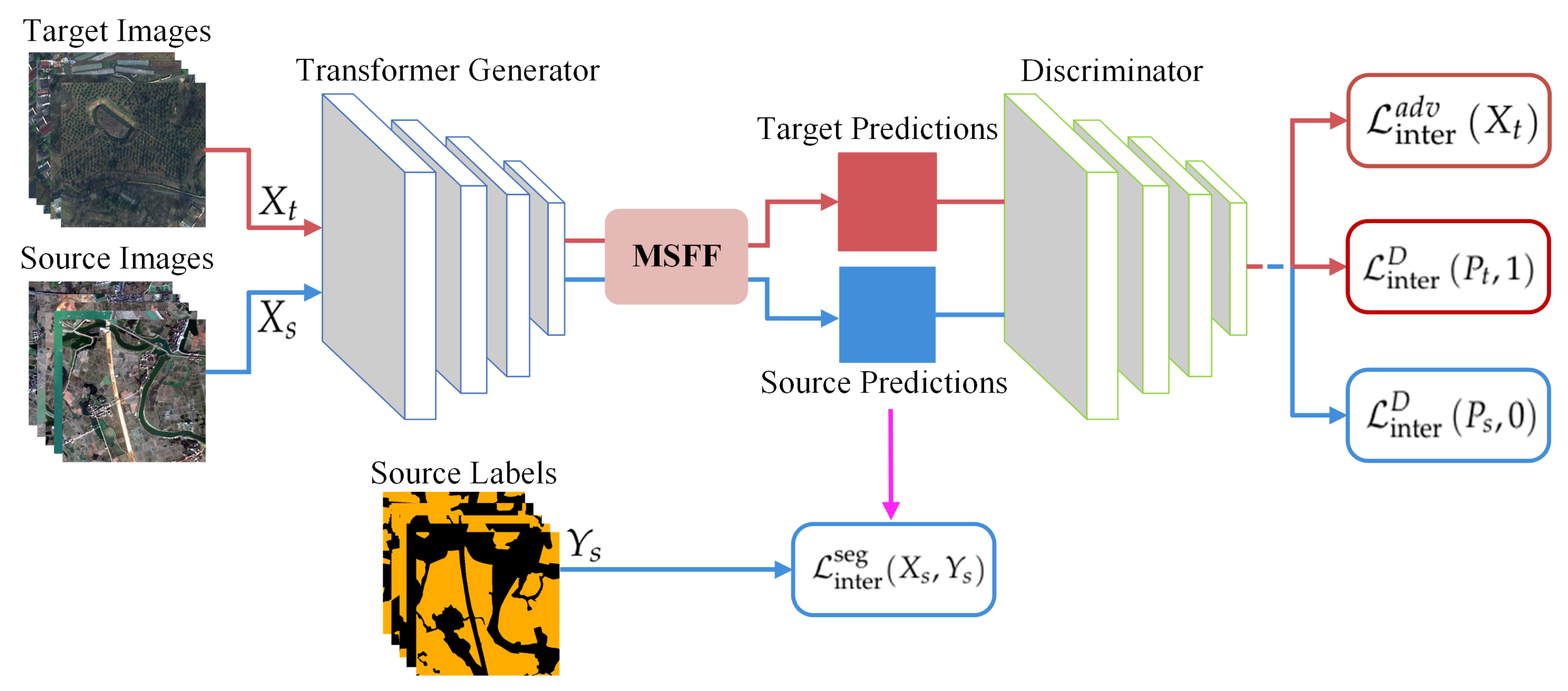
Interdomain adversarial adaptation is performed by training a generator (segmentation network) and a discriminator (fully convolutional network). The inter-domain generator and discriminator are denoted as G inter , D inter , respectively. After interdomain adversarial adaptation, we end up with a generator that can distribute the data similarly to the labeled and unlabeled images. The input source images and labels are denoted as X s ,   Y s , where X s R H × W × 3 , Y s ( 0 , 1 ) H × W (0 on behalf of the background pixels, 1 on behalf of the agricultural land pixels). The input target images without labels are denoted as X t , where X t R H × W × 3 . The prediction possibility maps obtained by the generator for the source and target images are denoted as P s ,   P t , respectively. P s = G inter X s ,   P t = G inter X t , where P s ,   P t R H × W × 2 .
The previous unsupervised domain adaptation methods [35,36,37,38] use resnet101 [42] as the backbone network to accomplish domain gap alignment. Inspired by the powerful long-range dependency modeling capability of the swin transformer [43], we use the hierarchical transformer as our generator backbone.
In the domain adaptation adversarial training process, the generator receives training samples from the source and target domains and outputs the corresponding predictions P s , P t . The purpose of the generator is to trick the discriminator, which learns features similar to those in the source and target domains. The purpose of the discriminator is to determine whether the input data are from the source or target domain. The domain labels of the source and target domain are, respectively, set to 0 and 1. The discriminator is used to determine the domain labels of the input feature maps. The discriminator calculates the generator’s output with its corresponding domain labels by the binary cross-entropy loss function. During training, the generator and discriminator are alternately trained to update the network parameters. Figure 2 shows the detailed inter-domain adaptation framework.
In the interdomain adaptation, as shown in Equation (1), the generator losses consist of an inter-domain supervised segmentation loss from the source images and an adversarial loss from the target images. Parameter λ inter is used to balance the two losses.
L inter G X s , X t = L inter s e g X s , Y s + λ inter L inter a d v X t
We can optimize the segmentation loss on the labeled source domain in a supervised manner by cross-entropy loss. The segmentation loss is formulated as follows:
L inter seg X s , Y s = h , w , c Y s ( h , w , c ) log G inter X s ( h , w , c ) ,
where Y s are transformed to one-hot vectors, and C represents the number of categories. However, the target domain does not have labels as supervised information, and using Equation (2) is not feasible for the loss calculation of the target domain samples. Therefore, we use the G inter obtained by training on the source domain to generate target domain image predictions. The discriminator receives the predictions from the target domain and outputs the predicted domain label. We artificially set the domain label of the target domain and calculate the loss of the predicted target domain label with the artificially set domain label by binary cross-entropy loss. The generator learns domain invariant features by optimizing the adversarial loss, the origin adversarial loss is formulated as follows:
L inter a d v X t = h , w t log D inter G inter X t ( h , w ) + ( 1 t ) log 1 D inter G inter X t ( h , w ) .
The target and source domains are as similar as possible to the feature mapping generated by the generator. Here, we set the target domain label to be the same as the source domain (domain label 0). We set t=0, and Equation (4) yields the final adversarial loss.
L inter a d v X t = h , w log 1 D inter G inter X t ( h , w )
For the discriminator, the discriminator loss consists of source and target domain discriminative loss. The discriminator must have good discriminatory power to determine the correct domain label for the input feature mapping. The discriminator loss is formulated as follows:
L inter D P s , P t = h , w s log D inter G inter X s ( h , w ) + ( 1 s ) log 1 D inter G inter X s ( h , w ) h , w t log D inter G inter X t ( h , w ) + ( 1 t ) log 1 D inter G inter X t ( h , w ) .
Forecasts for the source and target domains should approximate the corresponding domain labels. Here, we set the source domain’s domain label to 0 and the target domain’s domain label to 1 (s = 0, t = 1). The final inter-domain discriminator loss is shown in Equation (6).
L inter D P s , P t = h , w log 1 D inter G inter X s ( h , w ) h , w log D inter G inter X t ( h , w )

3.3. Intradomain Adaptation

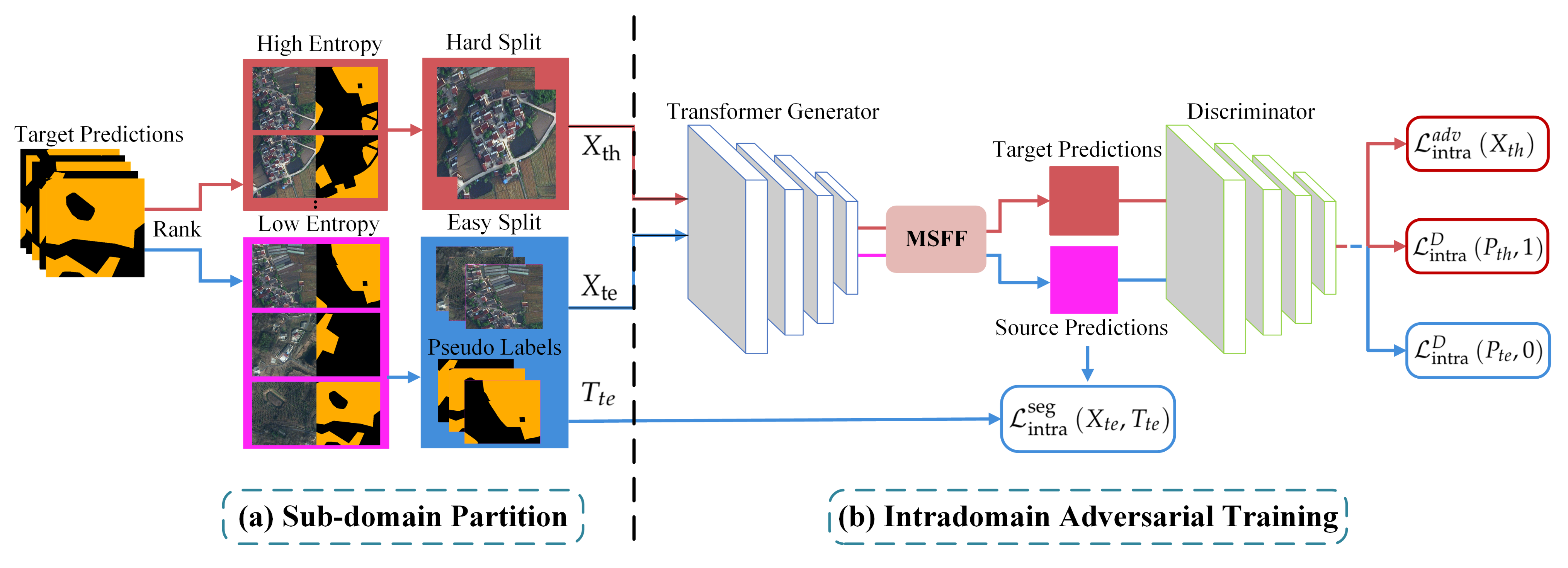
There are intradomain gaps in unlabeled images as a result of different regions, imaging angles, etc. Therefore, we further reduce the gap by intra-domain adversarial training on top of inter-domain adaptation. Figure 3 shows the detailed framework of the intra-domain adaptation. Intradomain adaptation includes two steps: sub-domain partition and intradomain adversarial training. The purpose of the sub-domain partition is to construct two sub-domain datasets to form the adversarial training, and the partition is achieved by entropy-based ranking. Intra-domain adversarial training aims to learn domain invariant features between the two sub-domains and eventually reduce the intra-domain variance. Generator and discriminator networks for the intradomain adaptation phase are consistent with the inter-domain ones.

3.3.1. Sub-Domain Partition

Since the target domain images are not labeled, we cannot directly train the unannotated images. Here, we divide the target domain by calculating the predicted entropy value of the unannotated images. The generator uses a supervised approach to the annotated images to obtain predictions with high confidence. The segmentation model obtained on the annotated images gives low-confidence predictions on the predicted unannotated images. The high certainty predictions represent the low entropy state, and the low prediction confidence represents the high entropy state. We divide the target domain images with high prediction confidence based on the entropy value and generate the corresponding pseudo labels. The entropy map I t is defined in Equation (7) as:
I t ( h , w ) = c P t ( h , w , c ) · log P t ( h , w , c ) ,
where · stands for Hadamard product. The confidence score R X t is the mean value of the entropy map, as shown in Equation (8):
R X t = 1 H W h , w c I t ( h , w , c ) .
Based on the prediction confidence scores, we divide the target domain images into hard split X th and easy split X te . We set a hyperparameter λ to control the division ratio, where X te = λ X t , X th = ( 1 λ ) X t . The effects of different hyperparameter settings on the experimental results are discussed in the discussion part.
The target domain is divided into an easy split source domain and a hard split target domain. Since the easy split subdomain contains images with high prediction confidence, we use a generator trained in the inter-domain adaptation phase to generate their corresponding pseudo-labels T t e , where T t e = G inter X t e .

3.3.2. Intradomain Adversarial Training

The intra-domain generator and discriminator are denoted as G intra , D intra , respectively. In the intra-domain adaptation, the prediction possibility maps obtained by the generator for the easy split subdomain and hard split subdomain images are denoted as P t e , P t h respectively. P t e = G intra X t e , P t h = G intra X t h , where P t e , P t h R H × W × 2 . We set the true domain labels of the easy split source domain and the hard split target domain to 0 1, respectively. In the intra-domain adaptation phase, the model structure is the same as in the inter-domain adaptation phase. The generator parameters are implemented by updating the intra-domain segmentation and adversarial loss. Parameter λ intra is used to balance the two losses.
L intra G X t e , X t h = L intra s e g X t e , T t e + λ intra L intra a d v X t h
In the same way as inter-domain adaptation, we use cross-entropy loss to train an easy split subdomain within a domain and their pseudo-labels using a supervised approach.
L intra seg X t e , T t e = h , w , c T t e ( h , w , c ) log G intra X t e ( h , w , c ) .
The adversarial loss is shown in Equation (11):
L intra a d v X t h = h , w log 1 D intra G intra X th ( h , w ) .
The discriminator receives training samples and determines their domain labels, we set s = 0, t = 1, and the intra-domain discriminator loss is formulated as:
L intra D P t e , P t h = h , w log 1 D intra G intra X t e ( h , w ) h , w log D intra G intra X t h ( h , w ) .

3.4. Multi-Scale Feature Fusion Module

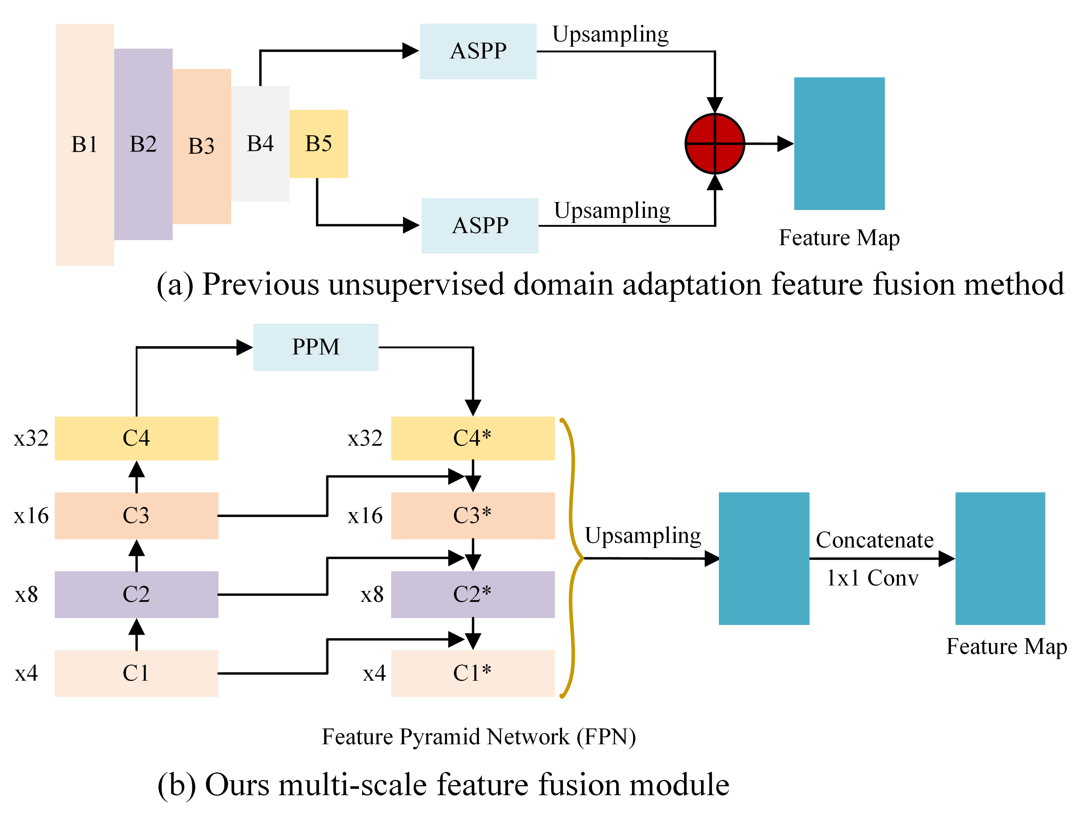
In the supervised methods of agricultural land segmentation [11,12,21,44], scholars focus on designing effective modules to fuse features at different scales. In the unsupervised domain adaption, the features extracted by the generator affect the final training result. The previous unsupervised domain adaptation methods [34,35,36,37,38,39] use resnet101 to extract domain invariant features. The features of the different layers extracted by resnet101 are denoted as B 1 , B 2 , B 3 , B 4 , B 5 . We use swin transformer [43] as our backbone of the generator, and C 1 , C 2 , C 3 , C 4 represents different layer features that the transformer backbone extracted. This is different from IntraDA [38]—they only consider using the last two layers of resnet101 features B 4 and B 5 , which may not be suitable for our agricultural land segmentation task.
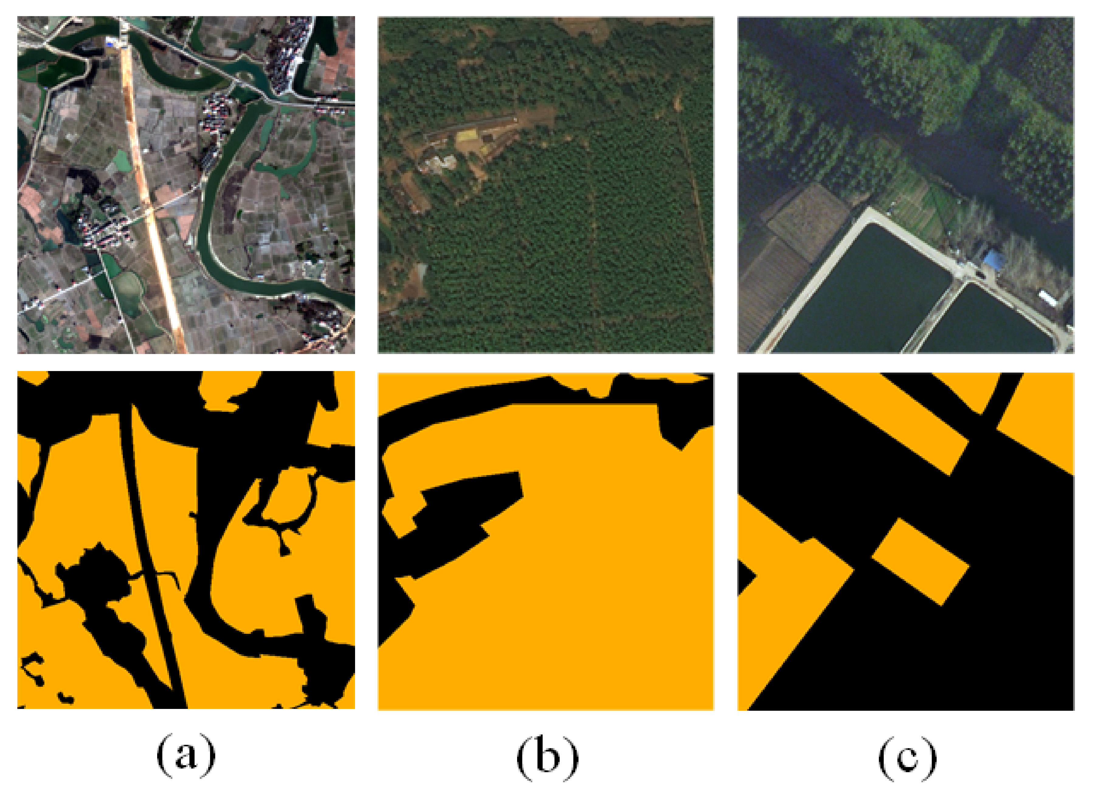
As shown in Figure 4, GID, DeepGlobe, and LoveDA are three datasets with different spatial resolutions and ground truth, which are 4 m/pixel, 0.5 m/pixel, and 0.3 m/pixel, respectively. Different spatial resolution datasets can complement each other in the domain adaptation task. The agricultural land coverage is comprehensive in the high spatial resolution dataset DeepGlobe. There are fewer heterogeneous regions in the images, making it difficult for the generator to extract discriminative features. The images in the low spatial resolution dataset GID represent a much wider geographical area. The generator has some limitations in terms of acquiring local features. Considering only the last two depth features of the generator may not be suitable for datasets with different spatial resolutions. We fuse the output features of all layers (i.e., C 1 , C 2 , C 3 , C 4 ) to extract domain invariant features.
Unlike [34,35,36,37,38,39], which upsample B 4 and B 5 features to the original image size separately and calculate their corresponding losses and gradients separately, we directly fuse the features of the four stages of the backbone network as the final output and calculate the gradient of the loss. Figure 5 depicts our multi-scale feature fusion module. First, we feed the output C 4 of the last layer of the backbone network into the Pyramid Pooling Module (PPM) [10] to obtain the tensor C 4 * with shape H 32 × W 32 × C * ( C * is set to 256 by default, H , W represent the height and width of the image, respectively). The PPM module allows global contextual information to be retained at different scales through multi-scale pooling operations. We then feed C 4 * into the Feature Pyramid Network (FPN) [41]. Specifically, we use 1 × 1 convolution to keep the number of C 4 * channels the same as C 3 and sum the upsampled C 4 * features to obtain the feature C 3 * . This process is repeated three times and the final features C 1 * , C 2 * , C 3 * , C 4 * with shapes H 4 × W 4 × C * , H 8 × W 8 × C * , H 16 × W 16 × C * , H 32 × W 32 × C * . By adaptive fusion of four scale features, the extracted features can be adapted to datasets with different spatial resolutions. Then, we upsample the features to the size of the original image and concatenate the four features in the channel dimension. Finally, we output the tensor of H × W × C using 1 × 1 convolution (for our binary classification task, C is set to 2) and obtain the final predicted probability map by the softmax function.

4. Experiments

4.1. Dataset Description

The GID dataset [21] is a large-scale land cover dataset constructed by the GF-2 satellite. The dataset consists of 150 finely labeled images, including 120 images in the training set and 30 images in the test set, each with a spatial resolution of 6800 × 7200, containing five categories: building land, farmland, forest, meadow, and water. Images from more than 60 Chinese cities are included in the dataset, which spans an area larger than 50,000 square kilometers. In addition, the dataset is also multi-temporal, collecting images from the exact location at different periods. These features determine a more complex data distribution of the GID dataset, representing more general agricultural land characteristics, which is advantageous for unsupervised domain adaptation tasks. There have been many studies using the GID dataset to conduct research related to classes of interest [45,46,47]. Similar to [12], we constructed a bi-partition dataset for agricultural land based on the GID RGB dataset, treating feature classes other than agricultural land as background pixels. The dataset can be found at https://captain-whu.github.io/GID/ (accessed on 18 June 2022).
The DeepGlobe dataset [22] is the first land cover classification dataset that provides sub-meter resolution. The dataset includes 1146 finely labeled RGB satellite images with a spatial resolution of 2448 × 2448. In our experiments, agricultural land is extracted as the category of interest, and the others are regarded as background pixels. The dataset is accessible at http://deepglobe.org/index.html (accessed on 30 July 2022).
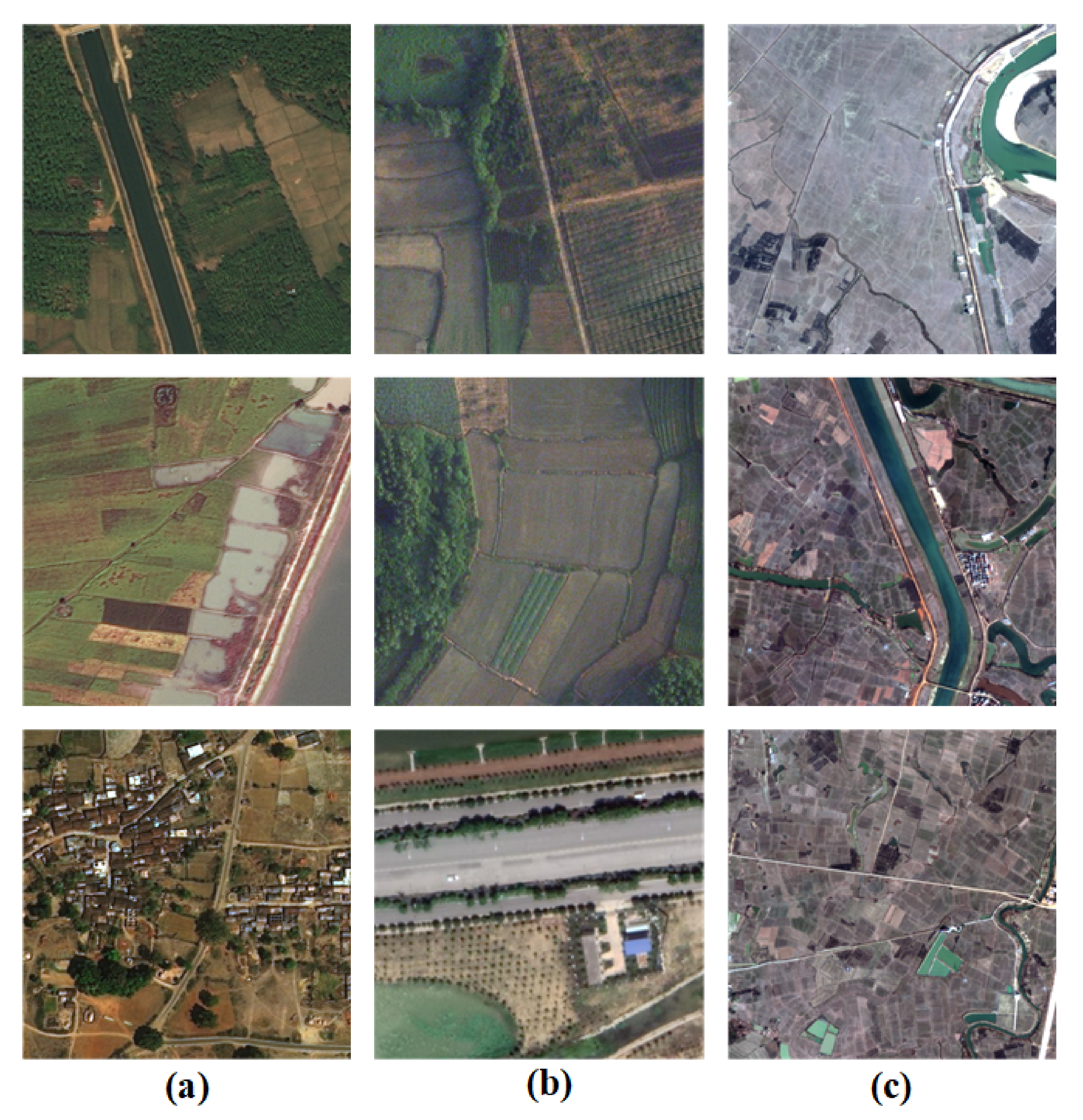
The LoveDA dataset [23] is a remote sensing dataset for unsupervised domain adaptation semantic segmentation tasks in remote sensing. Unlike other datasets that focus more on learning better models, LoveDA focuses on investigating the portability of network models. The dataset includes both urban and rural scenes, including 2713 images of the urban area and 3274 images of rural areas. LoveDA contains scenes more representative of general characteristics, which is advantageous for exploring unsupervised domain adaptive methods. The dataset is available at https://github.com/Junjue-Wang/LoveDA (accessed on 3 August 2022). Figure 6 displays a few images of the three datasets.

4.2. Data Processing

Since the original remote sensing image size is too large to feed directly into the network for training, we need to choose a suitable image size. Considering that agricultural use has broad coverage in the image, too small an image size ( 256 × 256 ) will result in the whole image being agricultural pixels, and the model will have difficulty learning discriminative features. Due to the limit of computer equipment, the generative adversarial network cannot train too large an image size of 1024 × 1024 . For the above considerations, we chose 512 × 512 as the input size for the model, a process that is cropped offline before feeding into the model. We take the same randomly generated 512 × 512 patch for the three datasets and then remove the images with less than 15,000-pixel points in agricultural land and background to finalize the dataset construction. 150 GID original datasets of 6800 × 7200 are processed to obtain 73490 source domain training images of 512 × 512 and their labels. When the GID dataset is used as the target domain, we randomly select 734 images for test evaluation. The DeepGlobe original dataset is 1146 images of 2448 × 2448 size, and 30,470 source domain training sets and their labels are obtained after processing. The LoveDA original dataset is 5987 data sets of 1024 × 1024 size, and 16,153 images are finally processed. 15,829 images are randomly chosen from this group to serve as the training set and 324 images as the test set. Table 1 displays the specific information of the datasets.

4.3. Evaluation Metrics

To quantitatively compare our unsupervised domain adaptive method with other methods, we use four evaluation metrics, intersection-over-union (IoU), COM, correctness (COR), and F1 score. Higher values for evaluation indicators mean better model results. IoU represents the predicted correct agricultural land pixels divided by the union of the true and predicted values of agricultural land pixels. COM represents the ratio of correctly predicted agricultural land pixels to actual agricultural land pixels. COR indicates the percentage of correctly predicted agricultural land pixels compared to all predicted agricultural land pixels. The F1 score represents the harmonic mean of COM and COR. Details of the evaluation indicators are shown as follows:
IoU = TP TP + FN + FP
COM = TP TP + FN
COR = TP TP + FP
F 1 = 2 × COM × COR COM + COR
where TP is the number of true positive pixels, FP is the number of false positive pixels and FN is the number of false negative pixels.

4.4. Implementation Details

In our generator, we use the swin transformer as our backbone network. Our discriminator uses a fully convolutional neural network consisting of five convolutional layers. A LeakyRule activation function follows the first four layers of the discriminator to augment the non-linear representation, and the last convolutional layer is used for the domain classifier. The initial learning rates of the generator and discriminator are each set to 4 × 10 6 , 4 × 10 7 . We use stochastic gradient descent (SGD) and Adam optimizer to update the parameters of the generator and discriminator, respectively. We set the maximum training iteration to 30,000 and use the poly learning rate decay strategy. Parameters λ inter and λ intra are set to 0.0001 and 0.001, respectively. The target domain images are divided into training and test sets. The training set consists of unlabeled data. The test set contains, in addition to images, corresponding labels for the model to evaluate performance in unsupervised domain adaptive methods. During the unsupervised domain adaption training process, the source domain images and the target domain training set are involved in the training. The final model training results are evaluated on a test set in the target domain. Our experiments are based on the Pytorch deep learning framework, and each experiment is repeated five times, and the average is taken as the result. Our experiments are performed on Ubuntu 18.04 with an RTX 3060 graphics card. With batch size set to 4 and training image size set to 512 × 512, 10,000 iterations take 14 h to train.

4.5. UDA Results on Different Adaptation Setting

We compared our unsupervised domain adaptive agricultural land extraction method with other methods under different source and target domain settings. As shown in Table 2, we set the source domain as the DeepGlobe dataset and the target domain as the LoveDA dataset. Our method achieved the best results (55.763% IoU, 62.549% COR, 67.750% F1 score) compared to other methods using the resnet101 backbone network. ADVENT and AdaptSegNet only considered inter-domain adaptation, and our method had 6%, 7%, 4.5%, and 6.5% higher IoU, COM, COR, and F1 scores, respectively. In addition, we can achieve better performance improvement than IntraDA, which achieves inter-domain and intra-domain adaptation. The better performance is due to the transformer-based backbone network considering the contextual relationship of different domains and the fusion of features of all layers in the backbone network.
As shown in Table 3, we set the GID dataset as the source domain and LoveDA as the target domain. Compared to other adversarial training methods, our method achieves optimal performance. Compared with IntraDA, our method achieves better performance (5.2% higher IoU, 32% higher COM, and 6% higher F1 score). We argue that the features learned from the low spatial resolution source domain GID (4 m/pixel) represent the global dependencies of the agricultural land, and the more local features are learned from the high spatial resolution LoveDA (0.3 m/pixel). In the design of our generator, the transformer backbone network and multi-scale feature fusion can extract better global and local features. During the adversarial training process in the source and target domains, our method can learn the domain invariant features that can be good.
We set the high spatial resolution DeepGlobe dataset as the source domain and the low spatial resolution dataset GID as the target domain. Table 4 shows the results of our experiments. Our method achieves the best results (49.553% IoU, 88.545% COM, 62.439% F1 score). However, compared with the two previous unsupervised domain adaption experiments, the effect improvement in this experiment is insignificant. We believe that although the backbone network can capture long-range dependencies, it is difficult to obtain effective global features on high spatial resolution datasets of size 512 × 512 .
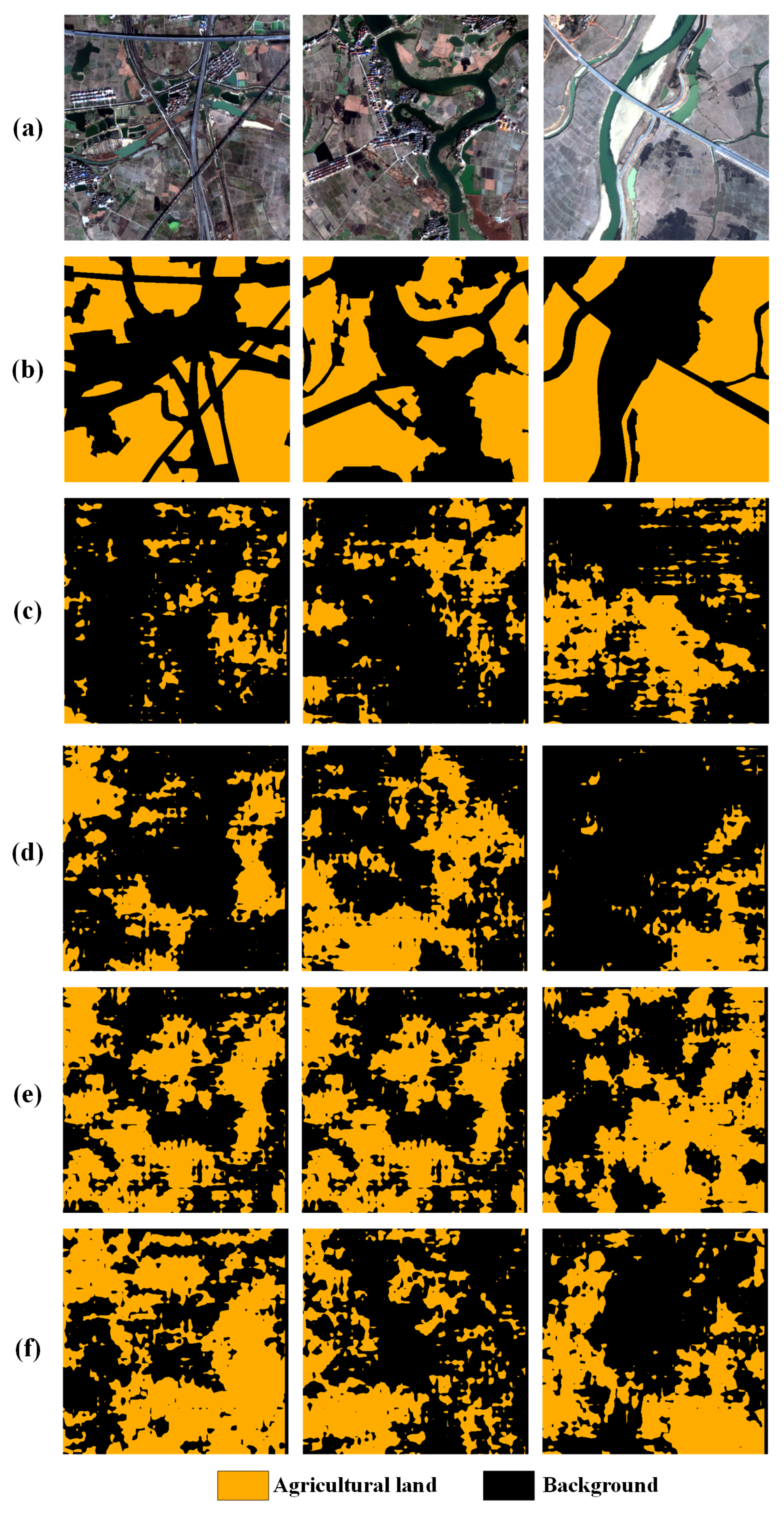
Figure 7c–f shows the visualization results, which are on the UDA setting DeepGlobe ⟶ GID using Source-only, ADVENT [36], IntraDA [38], and our method. When we do not use unsupervised domain adaptive methods, the predictions on the target domain are wrong due to the significant domain differences between the two domains. Significant domain differences affect our direct use of existing data, so we must use unsupervised domain adaptive methods to align domain differences to minimize a large amount of human data annotation.
Figure 7d–f show the segmentation prediction maps after using unsupervised domain adaptation. In the segmentation result map, there is a boundary blurring problem due to the large domain differences between the two cross-sensor datasets, which increases the difficulty of unsupervised domain adaptive methods in capturing domain invariant features. Our current model attempts to solve this problem by designing multi-scale feature modules to learn better domain invariant features. However, the visual prediction boundaries of the model are still relatively noisy. This suggests that the prediction uncertainty of the domain-invariant features learned by the generator on the target domain is still relatively large. However, compared to Figure 7c, the accuracy of agricultural land segmentation improves significantly. The unsupervised domain adaptation method can reduce the data annotation effort in practical application scenarios. Compared to ADVENT [36] and IntraDA [38], our method is closer to the actual label in qualitative visualization results. The transformer-based backbone network used in our approach can account for more long-range pixel dependencies, which is beneficial for agricultural land with a strong spatial correlation. In addition, our multi-scale feature fusion module considers the features of all layers of the backbone network, which can help the adaptive tasks in agricultural land scenes with different spatial resolutions.

5. Discussion

5.1. Comparative Methods

We used five methods to compare the performance of domain adaptation algorithms, namely, Source-only, AdapSegNet [35], ADVENT [36], BDL [37], IntraDA [38].
Souce-only means that we only use the source domain for training without making any domain adaptation on the target domain. In AdaptSegNet [35], Tsai et al. argued that the target and source domains share similar features and perform domain adaptation at the output layer through adversarial training. In ADVENT [36], Vu et al. observed a considerable uncertainty (high entropy) in predictions when models trained on the source domain migrated to the target domain, and they proposed the entropy-based loss to reduce the domain gap. In BDL [37], Li et al. proposed a bi-directional learning framework for unsupervised domain adaptive image segmentation. In IntraDA [38], Pan et al. proposed a two-stage entropy-based domain adaptation algorithm to address the problem that previous studies do not consider the differences in distribution within the domain. Unlike IntraDA, we used the transformer structure with more robust remote dependency modeling capabilities as the backbone network. We designed a multi-scale feature fusion module to accommodate remote sensing datasets of different spatial resolutions.

5.2. Ablation Study on Feature Fusion Method

We conducted ablation experiments on the setting of DeepGlobe ⟶ LoveDA, GID ⟶ LoveDA, DeepGlobe ⟶ GID. The baseline method is IntraDA [38], which adopts multi-level feature outputs. Our method used the transformer framework as the backbone to fuse proximal and distal features. And we designed the multi-scale feature fusion module (MSFF) to accommodate remote sensing datasets with different spatial resolutions. The final results of the ablation experiments are shown in Table 5.

5.3. Subdomain Division Factor

For the intra-domain adaptation phase, we divide the target domain into an easy split subdomain (with pseudo-labels) and a hard split subdomain based on the entropy of the target domain. We set the parameter λ from 0.5 to 0.9 and select the IoU metric as the evaluation criterion. As shown in Table 6, in DeepGlobe ⟶ LoveDA domain adaptation experiments, our method achieves the best results when λ = 0.8. In GID ⟶ LoveDA and DeepGlobe ⟶ GID domain adaptation experiments, our method achieves the best results when λ = 0.6.

5.4. Model Training

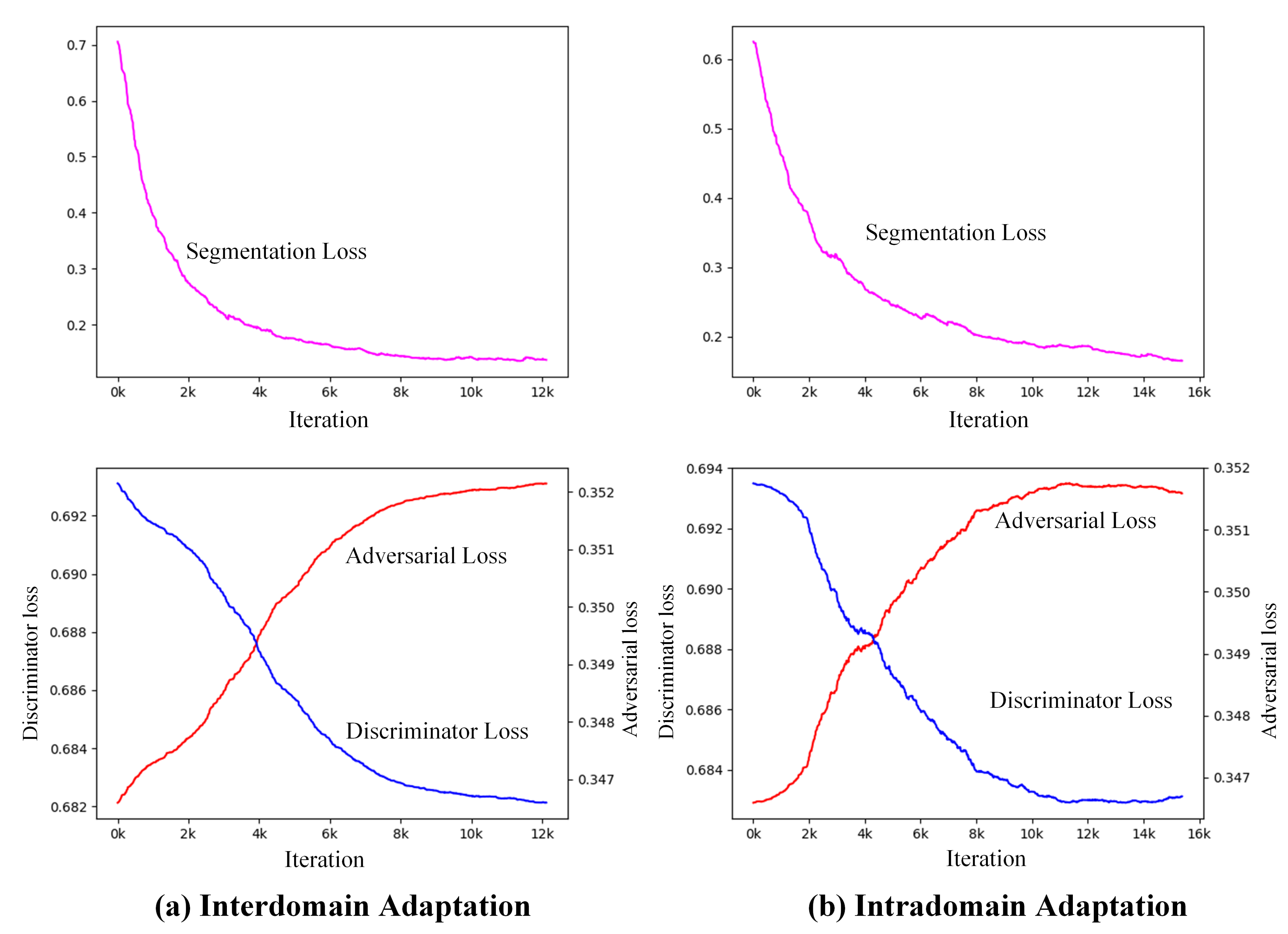
Figure 8 shows the variation curves of the loss during the intra-domain and inter-domain adaptation training. The generator learns the data distribution from the source domain in a supervised manner, and the segmentation loss decreases gradually throughout the training process. In the training process, the discriminator’s discriminative power gradually increases, and the adversarial loss in the target domain gradually increases. Finally, the discriminator loss and adversarial loss reach equilibrium when the generator learns the domain invariant features and completes the domain alignment.

6. Conclusions

In this work, we applied an unsupervised adversarial domain adaptation method to remote sensing images for agricultural land extraction. We first reduced the inter-domain gap by inter-domain adversarial training to obtain an adapted segmentation network. In the adversarial network generator, we used the transformer as the backbone. Meanwhile, we designed the multi-scale feature fusion module to cope with different spatial resolutions of the agricultural land dataset. Then, we predicted the target domain images based on the segmentation model obtained from inter-domain training and divided the target domain into subdomains based on entropy. Finally, we completed the intra-domain gap alignment by adversarial training between the sub-domains. Our model achieved better results on the remote sensing datasets of agricultural land. Our method can maximize the use of the existing annotated dataset to reduce the annotation cost on the unannotated datasets. In the next step, we will investigate more effective cross-sensor cross-scene domain adaptation methods and try to implement unsupervised agricultural extraction in realistic scenarios.

Author Contributions

Conceptualization, J.S. and J.Z.; methodology, J.Z. and J.S.; software, J.Z. and S.X.; validation, J.S. and X.W.; formal analysis, J.S., D.O. and M.W.; investigation, J.Z., J.S. and S.X.; resources, M.W.; writing—original draft preparation, J.Z. and S.X.; writing—review and editing, J.S., J.Z., D.O., X.W. and M.W.; visualization, J.Z. and S.X.; supervision, M.W.; project administration, M.W. and J.S.; funding acquisition, M.W. All authors have read and agreed to the published version of the manuscript.

Funding

This research was funded by research on intelligent monitoring and early warning technology for major rice pests and diseases of Sichuan Provincial Department of Science and Technology, grant number 2022NSFSC0172; Sichuan Agricultural University Innovation Training Programme Project Funding, grant number 202210626054.

Data Availability Statement

The data that support the findings of this study are available on request from the corresponding author.

Acknowledgments

The authors thank the anonymous reviewers for the helpful comments that improved this manuscript.

Conflicts of Interest

The authors declare no conflict of interest.

References

  1. Weiss, M.; Jacob, F.; Duveiller, G. Remote sensing for agricultural applications: A meta-review. Remote Sens. Environ. 2020, 236, 111402. [Google Scholar] [CrossRef]
  2. Alcantara, C.; Kuemmerle, T.; Prishchepov, A.V.; Radeloff, V.C. Mapping abandoned agriculture with multi-temporal modis satellite data. Remote Sens. Environ. 2012, 124, 334–347. [Google Scholar] [CrossRef]
  3. Matton, N.; Canto, G.S.; Waldner, F.; Valero, S.; Morin, D.; Inglada, J.; Arias, M.; Bontemps, S.; Koetz, B.; Defourny, P. An automated method for annual cropland mapping along the season for various globally-distributed agrosystems using high spatial and temporal resolution time series. Remote Sens. 2015, 7, 13208–13232. [Google Scholar] [CrossRef] [Green Version]
  4. Gebbers, R.; Adamchuk, V.I. Precision agriculture and food security. Science 2010, 327, 828–831. [Google Scholar] [CrossRef] [PubMed]
  5. Atzberger, C. Advances in remote sensing of agriculture: Context description, existing operational monitoring systems and major information needs. Remote Sens. 2013, 5, 949–981. [Google Scholar] [CrossRef] [Green Version]
  6. Boryan, C.; Yang, Z.; Mueller, R.; Craig, M. Monitoring us agriculture: The us department of agriculture, national agricultural statistics service, cropland data layer program. Geocarto Int. 2011, 26, 341–358. [Google Scholar] [CrossRef]
  7. Long, J.; Shelhamer, E.; Darrell, T. Fully convolutional networks for semantic segmentation. In Proceedings of the IEEE Conference on Computer Vision and Pattern Recognition, Boston, MA, USA, 7–12 June 2015; pp. 3431–3440. [Google Scholar]
  8. Ronneberger, O.; Fischer, P.; Brox, T. U-net: Convolutional networks for biomedical image segmentation. In Proceedings of the International Conference on Medical Image Computing and Computer-Assisted Intervention, Munich, Germany, 5–9 October 2015; pp. 234–241. [Google Scholar]
  9. Badrinarayanan, V.; Kendall, A.; Cipolla, R. Segnet: A deep convolutional encoder-decoder architecture for image segmentation. IEEE Trans. Pattern Anal. Mach. Intell. 2017, 39, 2481–2495. [Google Scholar] [CrossRef]
  10. Zhao, H.; Shi, J.; Qi, X.; Wang, X.; Jia, J. Pyramid scene parsing network. In Proceedings of the IEEE Conference on Computer Vision and Pattern Recognition, Honolulu, HI, USA, 21–26 July 2017; pp. 2881–2890. [Google Scholar]
  11. Lu, R.; Wang, N.; Zhang, Y.; Lin, Y.; Wu, W.; Shi, Z. Extraction of agricultural fields via dasfnet with dual attention mechanism and multi-scale feature fusion in south xinjiang, china. Remote Sens. 2022, 14, 2253. [Google Scholar] [CrossRef]
  12. Li, Z.; Chen, S.; Meng, X.; Zhu, R.; Lu, J.; Cao, L.; Lu, P. Full convolution neural network combined with contextual feature representation for cropland extraction from high-resolution remote sensing images. Remote Sens. 2022, 14, 2157. [Google Scholar] [CrossRef]
  13. Shang, R.; Zhang, J.; Jiao, L.; Li, Y.; Marturi, N.; Stolkin, R. Multi-scale adaptive feature fusion network for semantic segmentation in remote sensing images. Remote Sens. 2020, 12, 872. [Google Scholar] [CrossRef]
  14. Zhang, X.; Cheng, B.; Chen, J.; Liang, C. High-resolution boundary refined convolutional neural network for automatic agricultural greenhouses extraction from gaofen-2 satellite imageries. Remote Sens. 2021, 13, 4237. [Google Scholar] [CrossRef]
  15. Cordts, M.; Omran, M.; Ramos, S.; Rehfeld, T.; Enzweiler, M.; Benenson, R.; Franke, U.; Roth, S.; Schiele, B. The cityscapes dataset for semantic urban scene understanding. In Proceedings of the IEEE Conference on Computer Vision and Pattern Recognition, Las Vegas, NV, USA, 27–30 June 2016; pp. 3213–3223. [Google Scholar]
  16. Sen, L.I.; Ling, P.E.N.G.; Yuan, H.U.; Tianhe, C.H.I. Fd-rcf-based boundary delineation of agricultural fields in high resolution remote sensing images. J. Univ. Chin. Acad. Sci. 2020, 37, 483. [Google Scholar]
  17. Su, T.; Li, H.; Zhang, S.; Li, Y. Image segmentation using mean shift for extracting croplands from high-resolution remote sensing imagery. Remote Sens. Lett. 2015, 6, 952–961. [Google Scholar] [CrossRef]
  18. Graesser, J.; Ramankutty, N. Detection of cropland field parcels from landsat imagery. Remote Sens. Environ. 2017, 201, 165–180. [Google Scholar] [CrossRef] [Green Version]
  19. Hong, R.; Park, J.; Jang, S.; Shin, H.; Kim, H.; Song, I. Development of a parcel-level land boundary extraction algorithm for aerial imagery of regularly arranged agricultural areas. Remote Sens. 2021, 13, 1167. [Google Scholar] [CrossRef]
  20. Xue, Y.; Zhao, J.; Zhang, M. A watershed-segmentation-based improved algorithm for extracting cultivated land boundaries. Remote Sens. 2021, 13, 939. [Google Scholar] [CrossRef]
  21. Tong, X.-Y.; Xia, G.-S.; Lu, Q.; Shen, H.; Li, S.; You, S.; Zhang, L. Land-cover classification with high-resolution remote sensing images using transferable deep models. Remote Sens. Environ. 2020, 237, 111322. [Google Scholar] [CrossRef] [Green Version]
  22. Demir, I.; Koperski, K.; Lindenbaum, D.; Pang, G.; Huang, J.; Basu, S.; Hughes, F.; Tuia, D.; Raskar, R. Deepglobe 2018: A challenge to parse the earth through satellite images. In Proceedings of the IEEE Conference on Computer Vision and Pattern Recognition Workshops, Salt Lake City, UT, USA, 18–22 June 2018; pp. 172–181. [Google Scholar]
  23. Wang, J.; Zheng, Z.; Ma, A.; Lu, X.; Zhong, Y. Loveda: A remote sensing land-cover dataset for domain adaptive semantic segmentation. arXiv 2021, arXiv:2110.08733. [Google Scholar]
  24. Peng, D.; Guan, H.; Zang, Y.; Bruzzone, L. Full-level domain adaptation for building extraction in very-high-resolution optical remote-sensing images. IEEE Trans. Geosci. Remote Sens. 2021, 60, 1–17. [Google Scholar] [CrossRef]
  25. Ma, C.; Sha, D.; Mu, X. Unsupervised adversarial domain adaptation with error-correcting boundaries and feature adaption metric for remote-sensing scene classification. Remote Sens. 2021, 13, 1270. [Google Scholar] [CrossRef]
  26. Kwak, G.; Park, N. Unsupervised domain adaptation with adversarial self-training for crop classification using remote sensing images. Remote Sens. 2022, 14, 4639. [Google Scholar] [CrossRef]
  27. Zhang, L.; Lan, M.; Zhang, J.; Tao, D. Stagewise unsupervised domain adaptation with adversarial self-training for road segmentation of remote-sensing images. IEEE Trans. Geosci. Remote Sens. 2021, 60, 1–13. [Google Scholar] [CrossRef]
  28. Shamsolmoali, P.; Zareapoor, M.; Zhou, H.; Wang, R.; Yang, J. Road segmentation for remote sensing images using adversarial spatial pyramid networks. IEEE Trans. Geosci. Remote Sens. 2020, 59, 4673–4688. [Google Scholar] [CrossRef]
  29. Guo, J.; Yang, J.; Yue, H.; Liu, X.; Li, K. Unsupervised domain-invariant feature learning for cloud detection of remote sensing images. IEEE Trans. Geosci. Remote Sens. 2021, 60, 1–15. [Google Scholar] [CrossRef]
  30. Lu, X.; Gong, T.; Zheng, X. Multisource compensation network for remote sensing cross-domain scene classification. IEEE Trans. Geosci. Remote Sens. 2019, 58, 2504–2515. [Google Scholar] [CrossRef]
  31. Pan, S.J.; Tsang, I.W.; Kwok, J.T.; Yang, Q. Domain adaptation via transfer component analysis. IEEE Trans. Neural Netw. 2010, 22, 199–210. [Google Scholar] [CrossRef] [Green Version]
  32. Baktashmotlagh, M.; Harandi, M.T.; Lovell, B.C.; Salzmann, M. Unsupervised domain adaptation by domain invariant projection. In Proceedings of the IEEE International Conference on Computer Vision, Sydney, Australia, 1–8 December 2013; pp. 769–776. [Google Scholar]
  33. Shen, J.; Qu, Y.; Zhang, W.; Yu, Y. Wasserstein distance guided representation learning for domain adaptation. In Proceedings of the AAAI Conference on Artificial Intelligence, New Orleans, LA, USA, 2–7 February 2018; Volume 32. [Google Scholar]
  34. Hoffman, J.; Wang, D.; Yu, F.; Darrell, T. Fcns in the wild: Pixel-level adversarial and constraint-based adaptation. arXiv 2016, arXiv:1612.02649. [Google Scholar]
  35. Tsai, Y.-H.; Hung, W.-C.; Schulter, S.; Sohn, K.; Yang, M.; Chandraker, M. Learning to adapt structured output space for semantic segmentation. In Proceedings of the IEEE Conference on Computer Vision and Pattern Recognition, Salt Lake City, UT, USA, 18–23 June 2018; pp. 7472–7481. [Google Scholar]
  36. Vu, T.-H.; Jain, H.; Bucher, M.; Cord, M.; Pérez, P. Advent: Adversarial entropy minimization for domain adaptation in semantic segmentation. In Proceedings of the IEEE/CVF Conference on Computer Vision and Pattern Recognition, Long Beach, CA, USA, 15–20 June 2019; pp. 2517–2526. [Google Scholar]
  37. Li, Y.; Yuan, L.; Vasconcelos, N. Bidirectional learning for domain adaptation of semantic segmentation. In Proceedings of the IEEE/CVF Conference on Computer Vision and Pattern Recognition, Long Beach, CA, USA, 15–20 June 2019; pp. 6936–6945. [Google Scholar]
  38. Pan, F.; Shin, I.; Rameau, F.; Lee, S.; Kweon, I.S. Unsupervised intra-domain adaptation for semantic segmentation through self-supervision. In Proceedings of the IEEE/CVF Conference on Computer Vision and Pattern Recognition, Seattle, WA, USA, 13–19 June 2020; pp. 3764–3773. [Google Scholar]
  39. Chen, L.-C.; Papandreou, G.; Kokkinos, I.; Murphy, K.; Yuille, A.L. Deeplab: Semantic image segmentation with deep convolutional nets, atrous convolution, and fully connected crfs. IEEE Trans. Pattern Anal. Mach. Intell. 2017, 40, 834–848. [Google Scholar] [CrossRef] [Green Version]
  40. Xu, Z.; Zhang, W.; Zhang, T.; Li, J. Hrcnet: High-resolution context extraction network for semantic segmentation of remote sensing images. Remote Sens. 2020, 13, 71. [Google Scholar] [CrossRef]
  41. Lin, T.; Dollár, P.; Girshick, R.; He, K.; Hariharan, B.; Belongie, a.S. Feature pyramid networks for object detection. In Proceedings of the IEEE Conference on Computer Vision and Pattern Recognition, Honolulu, HI, USA, 21–26 July 2017; pp. 2117–2125. [Google Scholar]
  42. He, K.; Zhang, X.; Ren, S.; Sun, J. Deep residual learning for image recognition. In Proceedings of the IEEE Conference on Computer Vision and Pattern Recognition, Las Vegas, NV, USA, 27–30 June 2016; pp. 770–778. [Google Scholar]
  43. Liu, Z.; Lin, Y.; Cao, Y.; Hu, H.; Wei, Y.; Zhang, Z.; Lin, S.; Guo, B. Swin transformer: Hierarchical vision transformer using shifted windows. In Proceedings of the IEEE/CVF International Conference on Computer Vision, Montreal, BC, Canada, 11–17 October 2021; pp. 10012–10022. [Google Scholar]
  44. Zhang, D.; Pan, Y.; Zhang, J.; Hu, T.; Zhao, J.; Li, N.; Chen, Q. A generalized approach based on convolutional neural networks for large area cropland mapping at very high resolution. Remote Sens. Environ. 2020, 247, 111912. [Google Scholar] [CrossRef]
  45. Dang, B.; Li, Y. Msresnet: Multiscale residual network via self-supervised learning for water-body detection in remote sensing imagery. Remote Sens. 2021, 13, 3122. [Google Scholar] [CrossRef]
  46. He, C.; Li, S.; Xiong, D.; Fang, P.; Liao, M. Remote sensing image semantic segmentation based on edge information guidance. Remote Sens. 2020, 12, 1501. [Google Scholar] [CrossRef]
  47. Li, J.; Xiu, J.; Yang, Z.; Liu, C. Dual path attention net for remote sensing semantic image segmentation. Isprs Int. J. -Geo-Inf. 2020, 9, 571. [Google Scholar] [CrossRef]
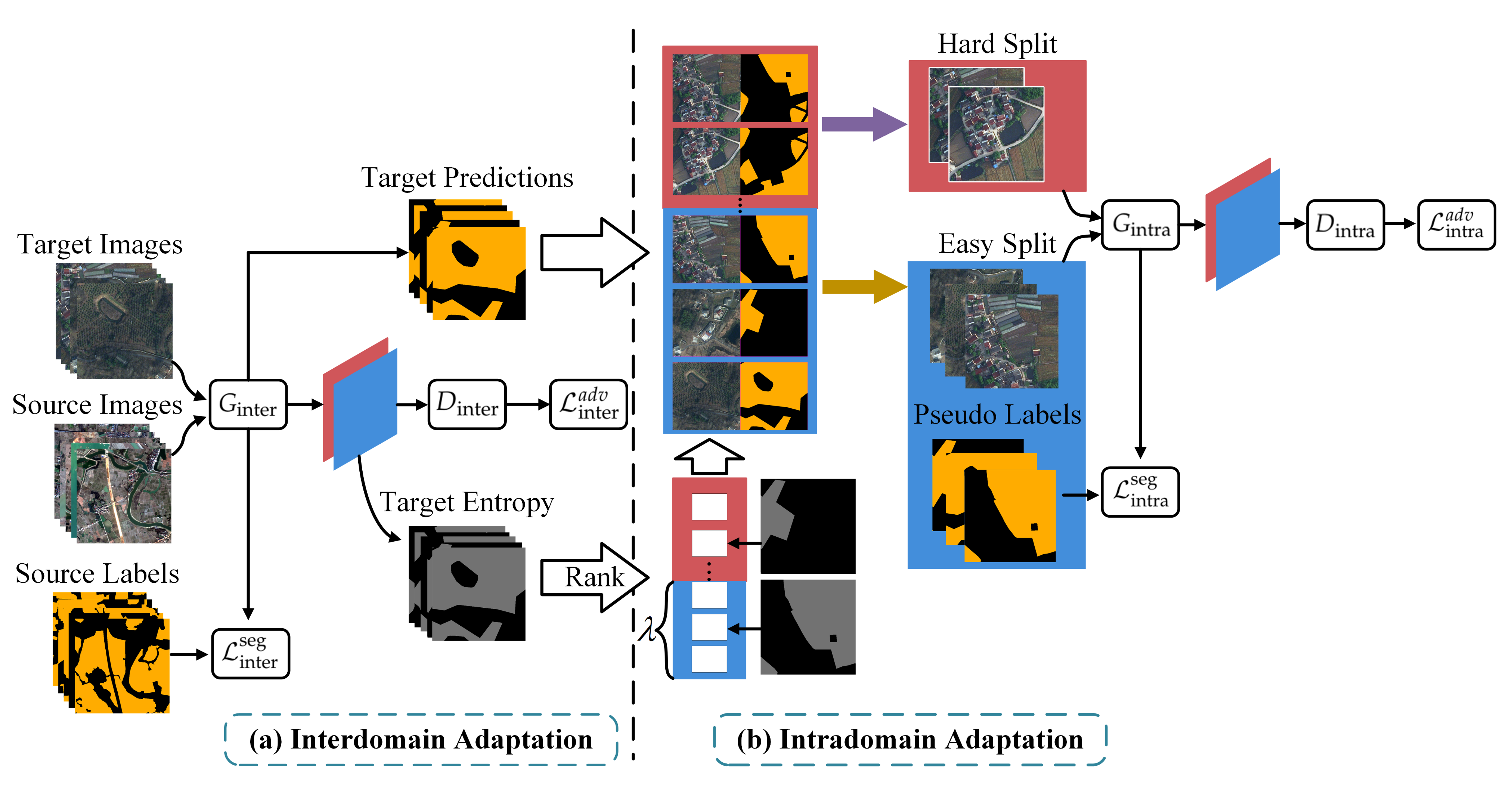
Figure 1. The general framework of our approach. In (a), the inputs are the images from the source domain with labels and the images from the target domain without labels; the outputs are optimised G inter and D inter . In (b), the inputs are easy split images (with pseudo labels) and hard split images (without labels); the outputs are optimised G intra and D intra .
Remotesensing 14 06298 g001
Figure 2. Interdomain Adaptation. The red line represents target domain data, and the blue line represents source domain data. The final outputs are optimised G inter and D inter .
Remotesensing 14 06298 g002
Figure 3. Intradomain Adaptation. The red line represents the hard split images, the blue line represents the easy split images. The final outputs are optimized G intra and D intra . (a) sub-domain partition; (b) intradomain adversarial training.
Remotesensing 14 06298 g003
Figure 4. Datasets with different spatial resolutions and their corresponding ground truth. (a) GID dataset with 4 m/pixel resolution; (b) DeepGlobe dataset with 0.5 m/pixel resolution; (c) LoveDA dataset with 0.3 m/pixel resolution.
Remotesensing 14 06298 g004
Figure 5. Multi-scale feature fusion module, ×4 means that the feature map resolution is one-fourth of the original image.
Remotesensing 14 06298 g005
Figure 6. Some samples of three agricultural land datasets. (a) DeepGlobe dataset with 0.5 m/pixel resolution; (b) LoveDA dataset with 0.3 m/pixel resolution; (c) GID dataset with 4 m/pixel resolution.
Remotesensing 14 06298 g006
Figure 7. Visualization of segmentation images with different methods. (a) Target image; (b) Ground truth dataset; (c) Source-only; (d) ADVENT; (e) IntraDA; (f) Ours.
Remotesensing 14 06298 g007
Figure 8. Loss variation during training when training our method on the setting GID ⟶ LoveDA. (a) Interdomain; (b) Intradomain.
Remotesensing 14 06298 g008
Table 1. The specific information of the datasets. The final image size fed to the network for training is 512 × 512 .
DatasetResolutionSensorOrigin SizeTraining DataTest Data
DeepGlobe0.5 m/pixelWorldView-2 2448 × 2448 30,470-
GID4 m/pixelGF-2 6800 × 7200 73,490734
LoveDA0.3 m/pixelSpaceborne 1024 × 1024 15,829324
Table 2. Experimental results on the setting of DeepGlobe ⟶ LoveDA.
DeepGlobe → LoveDA
MethodsIoUCOMCORF1
Source-only36.32745.89562.86149.108
AdaptSegNet [35]46.92174.47855.19060.404
ADVENT [36]49.39274.62158.08561.169
BDL [37]52.23479.74759.01165.334
IntraDA [38]51.71082.85557.34164.589
Ours55.76381.37062.54967.750
Table 3. Experimental results on the setting of GID ⟶ LoveDA.
GID ⟶ LoveDA
MethodsIoUCOMCORF1
Source-only36.22940.13983.01846.026
AdaptSegNet [35]42.93154.22171.29555.454
ADVENT [36]45.03560.76265.02158.250
BDL [37]44.59258.23167.44757.732
IntraDA [38]48.25460.36572.89860.799
Ours53.47092.10956.89166.042
Table 4. Experimental results on the setting of DeepGlobe ⟶ GID.
DeepGlobe ⟶ GID
MethodsIoUCOMCORF1
Source-only26.98639.20462.88436.599
AdaptSegNet [35]43.09868.61459.41456.067
ADVENT [36]45.99577.43557.40358.940
BDL [37]46.34875.78958.37359.508
IntraDA [38]47.63168.48860.29361.465
Ours49.55388.54554.53562.439
Table 5. Effectiveness analysis of the feature fusion method on the three unsupervised domain adaptation settings.
UDA SettingMethodIoUCOMCORF1
DeepGlobe ⟶ LoveDAbaseline51.71082.85557.34164.589
ours55.76381.37062.54967.750
GID ⟶ LoveDAbaseline48.25460.36572.89860.799
ours53.47092.10956.89166.042
DeepGlobe ⟶ GIDbaseline47.63168.48860.29361.465
ours49.55388.54554.53562.439
Table 6. Results of different hyperparameter λ settings of IoU on different datasets.
λ 0.50.60.70.80.9
DeepGlobe ⟶ LoveDA54.16054.44654.95355.76354.471
GID ⟶ LoveDA52.91353.47053.23152.55751.797
DeepGlobe ⟶ GID48.68549.55348.01248.19744.745
Publisher’s Note: MDPI stays neutral with regard to jurisdictional claims in published maps and institutional affiliations.