Article

LRFFNet: Large Receptive Field Feature Fusion Network for Semantic Segmentation of SAR Images in Building Areas

1
Aerospace Information Research Institute, Chinese Academy of Sciences, Beijing 100094, China
2
Key Laboratory of Technology in Geo-Spatial Information Processing and Application System, Chinese Academy of Sciences, Beijing 100190, China
3
School of Electronic, Electrical and Communication Engineering, University of Chinese Academy of Sciences, Beijing 101408, China
*
Author to whom correspondence should be addressed.
Remote Sens. 2022, 14(24), 6291; https://doi.org/10.3390/rs14246291
Submission received: 24 October 2022 / Revised: 4 December 2022 / Accepted: 9 December 2022 / Published: 12 December 2022
(This article belongs to the Special Issue SAR Images Processing and Analysis)

Abstract

:
There are limited studies on the semantic segmentation of high-resolution synthetic aperture radar (SAR) images in building areas due to speckle noise and geometric distortion. For this challenge, we propose the large receptive field feature fusion network (LRFFNet), which contains a feature extractor, a cascade feature pyramid module (CFP), a large receptive field channel attention module (LFCA), and an auxiliary branch. SAR images only contain single-channel information and have a low signal-to-noise ratio. Using only one level of features extracted by the feature extractor will result in poor segmentation results. Therefore, we design the CFP module; it can integrate different levels of features through multi-path connection. Due to the problem of geometric distortion in SAR images, the structural and semantic information is not obvious. In order to pick out feature channels that are useful for segmentation, we design the LFCA module, which can reassign the weight of channels through the channel attention mechanism with a large receptive field to help the network focus on more effective channels. SAR images do not include color information, and the identification of ground object categories is prone to errors, so we design the auxiliary branch. The branch uses the full convolution structure to optimize training results and reduces the phenomenon of recognizing objects outside the building area as buildings. Compared with state-of-the-art (SOTA) methods, our proposed network achieves higher scores in evaluation indicators and shows excellent competitiveness.

1. Introduction

Synthetic aperture radar (SAR) [1] is an active earth observation system and is not affected by light, climate, and clouds during the imaging process. The imaging resolution is independent of the flight height and can work around the clock. Synthetic aperture radar technology has become one of the most important methods of high-resolution earth observation [2]. The unique advantages of SAR make it widely used in various fields, such as ocean glacier monitoring, earth resource surveys, and crop identification [3].
The imaging geometry of SAR belongs to the oblique range projection type [4]. SAR images contain microwave characteristic information of ground objects and targets. The imaging results are affected by various factors, such as wavelength, incident angle, and polarization mode, and are closely related to the structure of the target, arrangement, and material. Therefore, SAR and optical images are very different in imaging mechanisms, geometric characteristics [5], radiation characteristics, and so on. These characteristics mentioned above leads to difficulty in extracting information from SAR images. Semantic segmentation technology can enhance the readability of SAR images [6].
In the SAR image semantic segmentation field, the commonly used traditional methods include support vector machine, decision tree, etc. [7]. Traditional methods use manually designed extractors for feature extraction [8]. Designing this type of method requires professional knowledge and a complex parameter adjustment process. At the same time, each method is only suitable for specific situations with poor generalization ability and robustness. In recent years, with the development of deep learning, neural networks have shown powerful image feature extraction capabilities [9]. Deep learning methods rely on data-driven feature extraction, which can obtain the feature representation of specific datasets through learning samples. The feature representations of datasets are more efficient and accurate, and the ability to extract features is more robust. The applications of deep learning to semantic segmentation of SAR images have just started and still have a lot of room for development [10]. Therefore, SAR image semantic segmentation based on the deep learning method can explore the feasibility of the deep learning method itself. On the other hand, it can explore what kind of network and which network structure is suitable for semantic segmentation [11].
The existing deep learning methods mainly deal with low-resolution, large-scale SAR images [12]. In low-resolution SAR images, unique characteristics, such as overlay, have little impact on the readability of the images. However, in high-resolution SAR images, these characteristics will significantly affect the readability of images. Figure 1 shows the contrast between an optical remote sensing image and a SAR image of the same area, and the enlarged part shows the image of high-rise buildings. It can be seen that there is an apparent overlapping phenomenon in the SAR image, and the boundary of buildings is not clear, which is difficult to distinguish. For the above reasons, semantic segmentation on high-resolution SAR images in building areas is more difficult than general semantic segmentation [13].
Therefore, we proposed a novel semantic segmentation framework for SAR images in building areas called the large receptive field feature fusion network (LRFFNet), which is composed of four parts: a feature extractor, a cascaded feature pyramid module (CFP), a large receptive field channel attention module (LFCA), and an auxiliary branch. SAR images contain single-channel information and have a low signal-to-noise ratio. If only low-level features are analyzed, it is difficult to accurately judge the representative category of pixels [14], we need to consider all level features at the same time and design a CFP model that can better capture contextual information. To solve the problem of locating key channels [15], we design an LFCA model. This module can judge the value of the channels and reassign the weights through the attention mechanism. It will give greater weight to the channel with more information. Our proposed channel attention mechanism can strengthen the importance of useful channels for segmentation tasks and suppress useless information, thus enabling the fast and accurate localization of useful channels. Due to the special imaging mechanism of SAR, different ground objects may have similar backscattering characteristics [16], so the identification of ground object categories is prone to errors. For this reason, we design an auxiliary segmentation branch to optimize the segmentation results and reduce segmentation errors.
Our main contributions are summarized below:
  • We design a network called LRFFNet that outperforms many SOTA works on the SAR semantic segmentation task.
  • The proposed CFP module can fuse multi-level features and improve the ability to capture contextual information.
  • The proposed LFCA module can reassign the channel weights, the channel with more information is given higher attention, the useless information is suppressed, and the ability to locate the channel containing key information is improved.
  • Our proposed auxiliary branch can restrict the network to perform segmentation within the building area and reduce the phenomenon of color blocks generated outside the building area and optimize the segmentation results.
The rest of this paper is organized as follows. Section 2 introduces the related work on the semantic segmentation of optical images and SAR images. Section 3 describes the overall framework and important components of LRFFNet. Section 4 details the experiments and analysis on the SARMV3D-BIS dataset. The conclusion of this paper is in Section 5.

2. Related Work

Semantic segmentation is an important direction of computer vision [17]. Unlike image classification, semantic segmentation achieves pixel-level classification of images [11]. Semantic segmentation is an output-intensive task. Semantic segmentation on SAR images can classify different regions into different categories, thereby assisting humans in understanding the image [18].

2.1. Traditional Approaches

Traditional methods do not rely too much on domain knowledge but use features designed manually, including pixel color [19] in different image spaces, histograms of oriented gradients [20], scale-invariant feature transform [21], bag of visual words [22], and so on. Based on these artificially designed features, many methods have been designed.
Although the result obtained is not strictly semantic classification in unsupervised segmentation, the content is recognized, and the image is divided by content. The k-means algorithm is one of the representative algorithms [23]. The process is randomly placing k centroids in the feature space, assigning data points to the centroids in the principle of proximity, and then gradually adding the centroids to the cluster. Another method is a graph-based image segmentation algorithm [24]. The core idea of this algorithm is to regard each pixel in the image as a vertex and use an indicator such as color difference as edge weights. A minimum spanning tree method is used to cut the edges. Fei et al. proposed a soft association strategy to make the clustering differentiable [25]. In this method, each pixel is assigned to various clusters with different probabilities. Bo et al. proposed DSFA for pixel-level tasks [26]. The author uses two symmetric deep networks project the input images and use the SFA process on the transformed features. To reduce the size of the involved optimization problems, Huang et al. proposed a scalable subspace clustering method [27]. The method integrates a concise dictionary and robust subspace representation. Other unsupervised methods include Active Contour Models [28], Watershed Segmentation [29], etc.
There are many representative algorithms in the field of supervised semantic segmentation. Random decision forests [30] is an ensemble learning method in which multiple classifiers are trained and used. The structure of the classifier is a decision tree, the leaves represent the categories, and the features are used to determine the branch direction. SVM [31] is a generalized linear classifier for the binary classification of data that converts the original problem into a convex quadratic programming problem and has a strong nonlinear fitting ability. When the original data are linearly separable, SVM finds the optimal classification hyperplane in the original space. When the original data are linearly inseparable, SVM will add slack variables to map the nonlinear data to a high-dimensional space and become linearly separable. In addition, there are methods such as Markov Random Fields [32], Conditional Random Fields [33], etc.

2.2. Deep Learning-Based Methods

With the development of deep learning in recent years, many excellent frameworks have been proposed and applied to semantic segmentation tasks.
Long et al. proposed the FCN semantic segmentation framework [34]. The network uses the deconvolution layer to upsample the feature map of the last layer. Then restore the feature map to the same size as the input image so that a prediction can be generated for each pixel. Unet [35] is a variant of the FCN structure and adopts a symmetrical network structure. The overall structure can be regarded as two parts. The first half is for feature extraction, the second half is for upsampling, and a jump connection structure is used to achieve retrieving edge features. EncNet [36] designs the context encoding module by adding the prior knowledge of the scene and uses semantic encoding loss to regularize the training of the features extracted by the module, which is more conducive to the training process. In APCNet [37], the authors found that GLA plays an essential role in constructing contextual features. Based on this, an ACM block was designed, and the final representation matrix at different scales was obtained by incorporating affinity coefficients. A more robust attention mechanism is proposed in EMANet [38], which extracts a more compact set of bases from the original features through the expectation maximization algorithm and reduces the computational complexity. The DeepLab series [39,40,41,42] use atrous spatial pyramid pooling to gather receptive fields of different scales and effectively expand the filter without increasing the number of parameters and computational complexity. In addition, the author introduces the multi-grid policy; that is, using atros convolution many times.
The PSPNet [43] proposed by Zhao et al. aggregates the context of different regions through the pyramid pooling module and the pyramid scene analysis network so that the model can understand the global context information. Fu et al. proposed DANet [44], which reconciled the relationship between local features and global dependencies by introducing a spatial attention mechanism, and a channel attention mechanism. CCNet [45] proposed by Huang et al., obtains the context information of the pixel through the intersection path of each pixel. Then, through a recurrent operation, each pixel can finally capture the whole image dependencies of all pixels. CGNet [46], proposed by Wu et al., is mainly composed of CG blocks. Residual learning is mainly used in the CG block, including local residual learning (LRL) and global residual learning (GRL). The CG block can provide the joint features of local features, and the surrounding environment context is learned. Finally, the learning of joint features is further improved by introducing global context features. In order to solve the problem of insufficient spatial resolution, BiSeNet [47] designs a small stride spatial connection path. To further expand the receptive field, a fast downsampling strategy is adopted to redesign the context path.
However, most semantic segmentation models are oriented toward optical images (which are obtained from the visible light band sensor). SAR adopts the side-view mode to transmit and receive radar waves, and the obtained images have a low signal-to-noise ratio, making it more difficult to distinguish the content. Applying these models directly to the SAR image semantic segmentation does not work well [48].
Wang et al. proposed and evaluated a deep neural network topology for the automatic segmentation of SAR images named HR-SARNet [49]. Ding et al. used parallel multiscale branches to improve the embedding of local discriminative features and proposed MP-ResNet [50]. Wu et al. adopted the fully convolutional network (FCN) and U-Net architecture and proposed the MS-FCN method [51]. Yue et al. built a multiscale attention model by using multiscale feature extraction, channel attention extraction, and spatial attention extraction [52]. They designed a loss function by combining lovasz-softmax and cross-entropy losses and proposed a novel attention fully convolutional network. Based on U-Net, He et al. added a global feature attention module to the decoder of U-Net, proposed a new semantic segmentation network IGFU-Net [53], and used it on SAR images. Semantic segmentation of urban and non-urban areas was achieved with better accuracy than U-Net. Cha et al. proposed a multimodal representation learning method for SAR semantic segmentation based on contrastive multi-view encoding [54], using EO images, SAR images, and label masks at the same time. Facing extremely imbalanced glacier data, Davari et al. used the Matthews Correlation Coefficient (MCC) as an early stopping criterion [55] while also improving the distance map-based Binary Cross Entropy (BCE) loss function. Bi et al. proposed a context-based method for the semantic segmentation of PSAR images [56]. Taking the channel-consistent feature set defined by the authors as input, the three-dimensional discrete wavelet transform (3D-DWT) technique is used to extract multiscale features that are robust to speckle noise. Then, a Markov Random Field (MRF) is applied during the segmentation process to enforce label smoothing spatially. The above techniques enable context information to be fully integrated into the segmentation process to ensure accurate and smooth segmentation.

3. Proposed Method

In this section, we first introduce the overall structure of our proposed network. Then we present the main components of the network, including the feature extractor, the cascaded feature pyramid module, the large receptive field channel attention module, and the auxiliary branch.

3.1. Overall Architecture

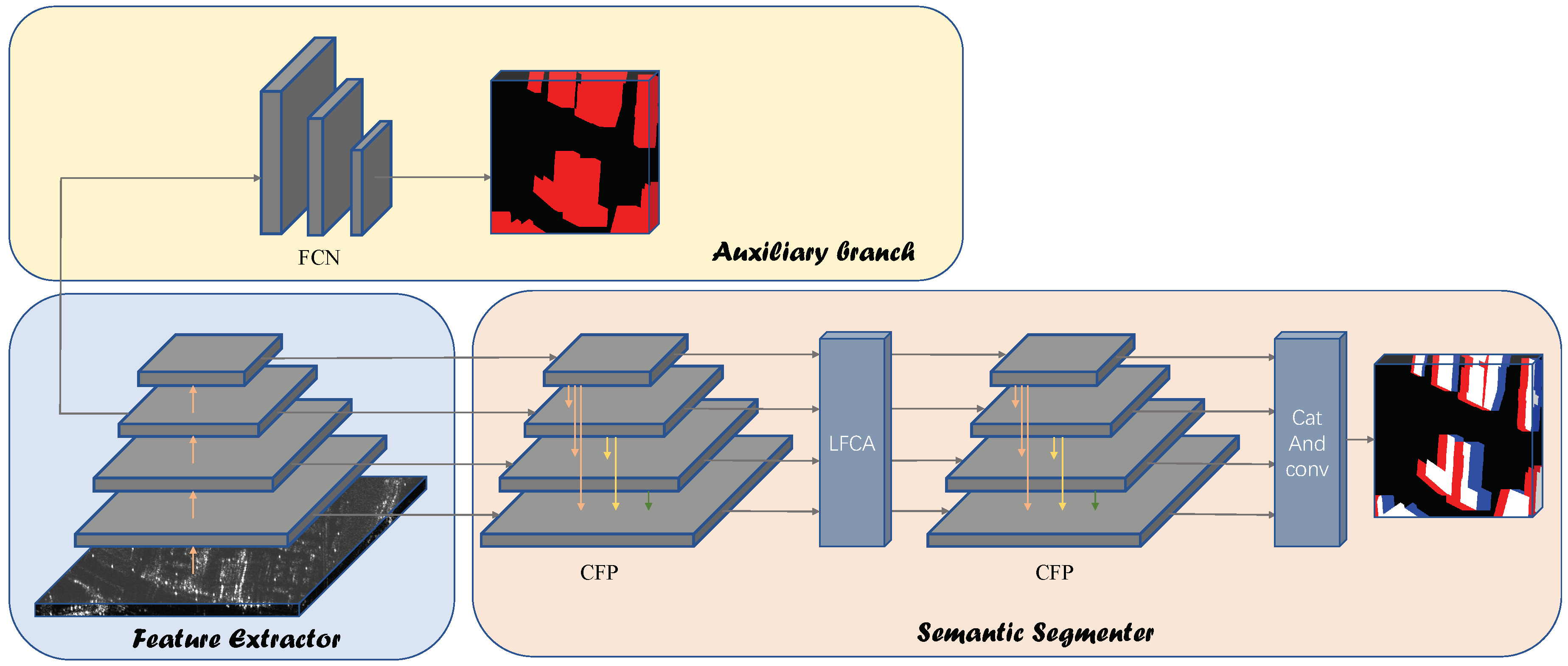
We propose a semantic segmentation method on the basis of the encoder-decoder architecture. As shown in Figure 2, our model can be divided into three parts according to different functions: a feature extractor, a semantic segmenter, and an auxiliary branch. The feature extractor is the encoder, through which the multi-level features can be extracted from the input image.
The feature extractor plays the encoder role. It can extract features from the input image. They are then sent to the semantic segmenter and the auxiliary branch. The role of the semantic segmenter is to recover feature resolution and generate pixel-level predictions. This structure mainly contains two cascade feature pyramid (CFP) modules and a large receptive field channel attention (LFCA) module. Optical images contain grayscale information about multiple visible light bands, while SAR images only contain information about the microwave band. In addition, SAR images have geometric distortion. Based on the above reasons, semantic segmentation on SAR images is more difficult. The feature maps obtained from the feature extractor have a total of 4 levels, from low-level to high-level. Low-level features contain more structural information, and high-level features contain more semantic information. If only one level of feature is used for segmentation, it is sufficient for optical images but not for SAR images. The CFP module can complete the fusion of all levels of features through multi-path connections. The LFCA module can help the network focus on the channel that is more favorable for the segmentation task. Considering that SAR images can be divided into building and non-building areas, and the identification of ground object categories is prone to errors, we propose the auxiliary branch. The FCN structure is used in this branch, which can optimize the network training effect and improve the quality of predicted images.

3.2. Feature Extractor

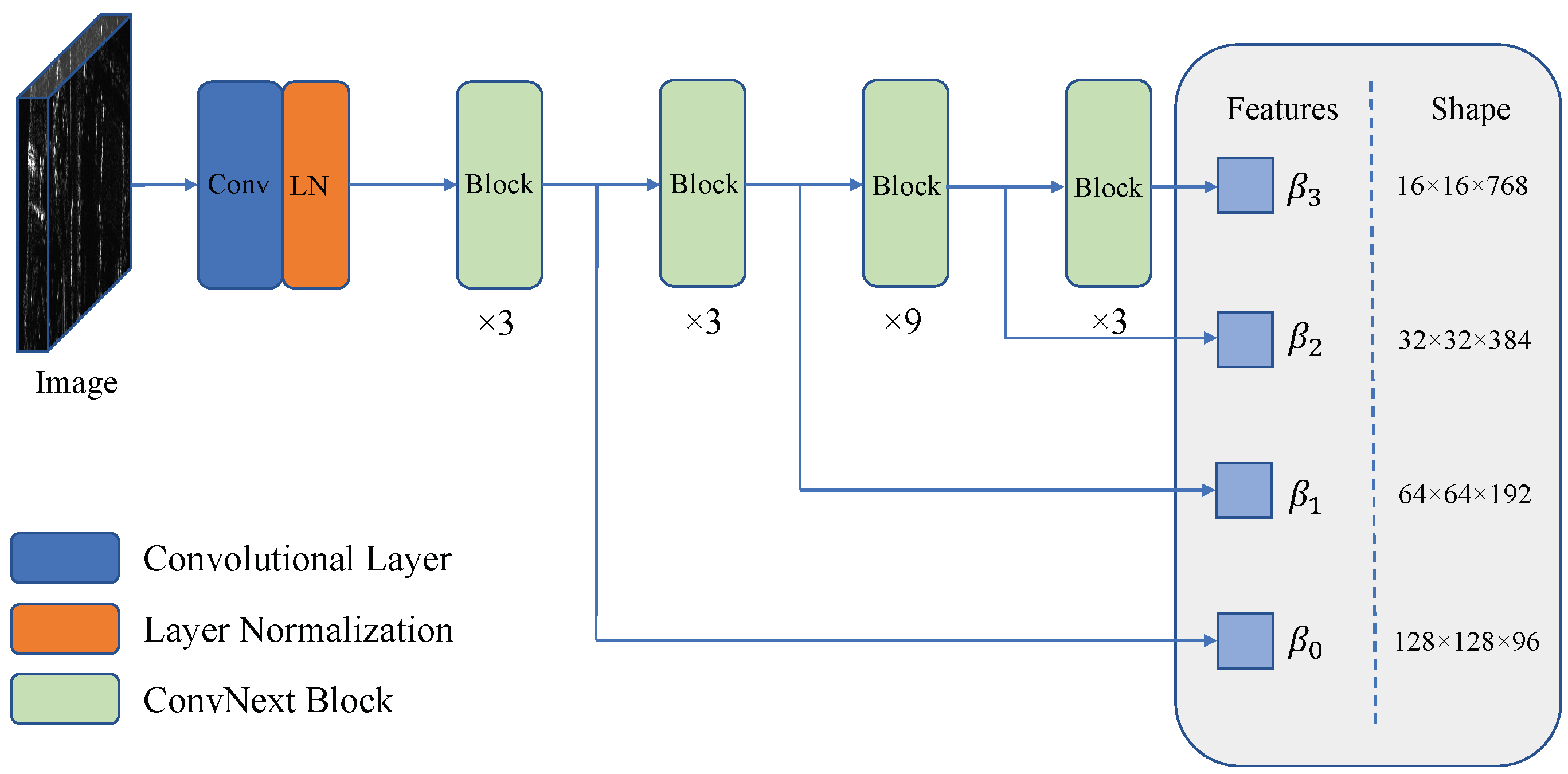
The feature extractor uses the ConvNeXt structure. This is a pure convolutional neural network proposed by Liu et al. [57], which achieves top-1 accuracy in the ImageNet segmentation task. The network structure is adjusted and improved on the basis of ResNet [58]. The proportion of each stage is improved in the macro design, using depthwise separable convolution, inverse bottleneck layer, etc. In the detailed design, the activation function in the network is changed from ReLu [59] to GELU [60], and fewer activation functions are used. ConvNeXt uses fewer normalization layers than ResNet, and the normalization layer used is LN [61] rather than BN [62]. The overall structure of the feature extractor is shown in Figure 3.
In the feature extractor, the input image first passes through a 4 × 4 convolution layer, then a normalization layer. After these two layers of processing, the image resolution becomes one-fourth of the original. Then the feature will be processed through a series of ConvNeXt Blocks. These ConvNeXt Blocks are divided into four parts, namely, four stages. Each stage contains 3 , 3 , 9 , 3 blocks. ConvNext Block contains depth-wise conv2d, layer normalization, GELU activation function, scale layers, and droppath layer, and these layers are connected in series. We did not modify the original network structure and parameters. The features extracted through the four stages are β 0 , β 1 , β 2 , β 3 , these features then enter the decoder layer to perform feature fusion and other operations to extract sufficient information.

3.3. Semantic Segmenter

The role of the semantic segmenter is to extract information from the multi-level features. The decoding operation is completed by recombining the feature layers to generate a semantically segmented image. We design an efficient structure to accomplish the generation of semantic segmentation images. The structure includes two cascaded feature pyramid modules (CFP) and a large receptive field channel attention layer (LFCA). The specific model structure can be seen in Figure 2.

3.3.1. Cascade Feature Pyramid Module

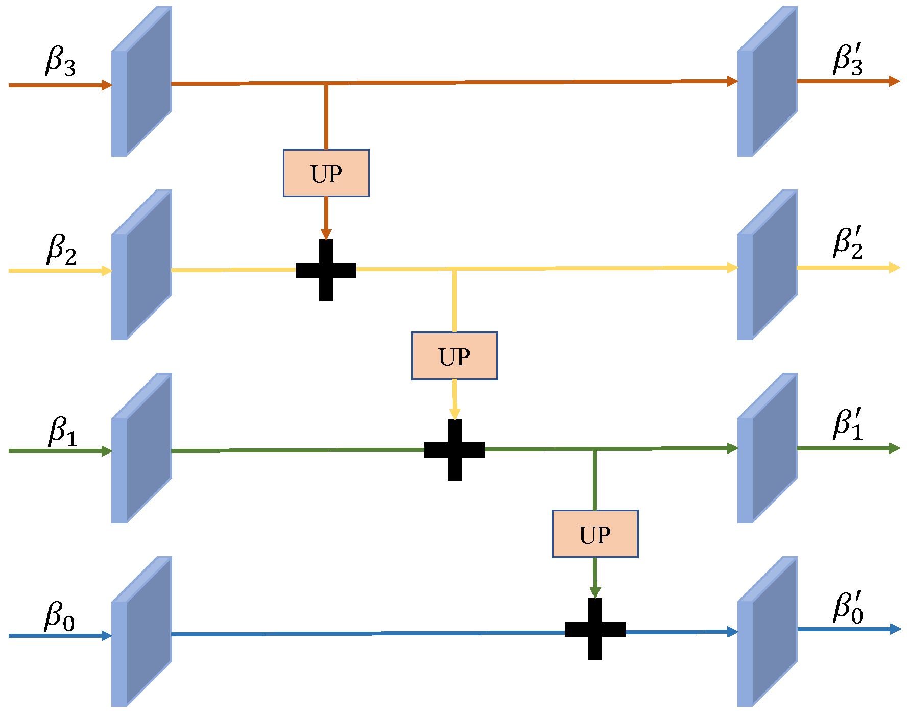
Feature Pyramid Networks (FPN) [63] involve constructing a series of images or features of different scales for model training and testing. Features at different levels contain information with different emphases; low-level features mainly reflect details such as light, shade, and edges, and high-level features have rich semantic information. The structure of FPN is shown in Figure 4, “UP” denotes the upsampling layer, which uses the bilinear interpolation method. After the upsampling operation and the feature addition operation, the low-level features can obtain high-level information. The use of low-level features alone cannot contain the overall structural information. The fusion of high-level features into low-level features takes into account the structural and semantic information at the same time. Meanwhile, the features fused through the FPN structure will have richer expression capabilities. This structure can improve the robustness of the segmentation algorithm for the segmentation performance of objects of different sizes. The single-path connection from high-level features to low-level features in FPN limits the ability of feature fusion. We design a multi-path connection method to improve the model and propose a CFP module. The structure of our proposed CFP is shown in Figure 5, “RE” denotes the upsampling layer, “ADD” denotes the element addition operation, and “CBR” denotes the series structure of the convolutional layer, BN layer, and activation function layer.
In the FPN structure, the underlying features are fused with the upper features through the upsampling method. The implementation of upsampling is the bilinear interpolation method. In addition to enlarging the size, the upsampling layer has almost no other effect. It even introduces unnecessary values due to the calculation method, which affects the calculation of subsequent features. In our model, we add a convolutional layer after the upsampling layer, which has a 1 × 1 kernel size. By doing so, the model can not only achieve the effect of enlarging the size of the feature but also achieves the adaptive filling of the feature value. The input to CFP is denoted as β 0 , β 1 , β 2 , β 3 , a total of four layers of features. After CFP layer processing, the output intermediate layer features are β 0 , β 1 , β 2 , β 3 . This process can be written as
β 0 = β 0 + f c b r f r e β 1 + f r e β 2 + f r e β 3 β 1 = β 1 + f c b r f r e β 2 + f r e β 3 β 2 = β 2 + f c b r f r e β 3 β 3 = β 3
where f c b r ( · ) represents a series of operations in the order of the 1 × 1 convolution, batch normalization, and ReLU activation function. f r e ( · ) represents the upsample operation, whose purpose is to resize the high-level features so that they can be added to the target feature layer. The specific method used by the upsampling layer is bilinear interpolation. For the top-level feature β 3 , we do not perform any calculation but keep the original value.
The features obtained after the processing of CFP are then processed by the LFCA model. Details of the computations performed in the LFCA model are in Section 3.3.2. After processing by the LFCA model, we obtained features β 0 , β 1 , β 2 , and β 3 . Then, the feature is processed by the second CFP, obtaining the features β 0 , β 1 , β 2 , and β 3 . We call the structure of two connected CFPs C-CFP. Then, we obtain the final semantic segmentation result map by
p r e d i c t = f d c ( f c b r ( β 0 f r e ( β 1 ) f r e ( β 2 ) f r e ( β 2 ) ) )
where f d c ( · ) means a series of operations in the order of the dropout and 1 × 1 convolution. f c b r ( · ) means a series of operations in the order of the 3 × 3 convolution, batch normalization, and ReLU activation function. f r e ( · ) means the upsample operation, and ⊕ represents concat operation.
It can be obtained from the equation that after the feature fusion layer, the features of the second level are fused with the features of the first level, the features of the third level are fused with the features of the second level, and the first level at the same time, and the fourth level of features are fused with the previous three levels of features at the same time. This connection method enhances the cross-layer information-sharing ability between different feature levels.

3.3.2. Large Receptive Field Channel Attention Module

Starting with SEnet [64], introducing a channel attention mechanism into convolution shows great potential for performance improvement. By judging the amount of information in the channel, different weight factors are assigned to different channels so the network can focus on more valuable channels. The general expression of the channel attention mechanism can be expressed as:
F = σ ( W Y )
where F is a weight factor to be multiplied to the different channels of the feature, which has a shape of ( c × 1 ) . σ is the activation function, and W is the weight matrix, which has a shape of ( c × c ) . Y is the set of features obtained from the previous process.
An advanced channel attention mechanism module is designed in EcaNet, and the name is the ECA module. This module implements the avoidance of dimensionality reduction operations that negatively affect the predictions of the channel attention mechanism. In the ECA module, the global average pooling layer and one-dimensional convolution are used to calculate the channel weights. The one-dimensional convolution layer used in the ECA module achieves effective cross-channel interaction. In the ECA module, the calculation process of the attention mechanism can be described as follows:
F = σ ( C 1 D K ( G A P ( Y ) ) )
where Y is the set of features obtained from the previous process. G A P ( · ) means global average pooling layer. C 1 D K means a one-dimensional convolution layer.
At the same time, we observed that the global average pooling operation is used to calculate the channel weight in Squeeze and Excitation Networks (SENet), style-based recalibration module (SRM), and Efficient Channel Attention Network (EcaNet), which limits the expressive ability of the model. The calculation process in ECAlayer can be summarized as follows: perform a global pooling operation on the input feature to obtain a one-dimensional feature vector, then perform a one-dimensional convolution on the one-dimensional vector to obtain the channel allocation weight, and then multiply the weight to the original feature to get the weighted features. In the original network, the global average value of the feature of each channel is used as the weight value. The result is that only global features are considered, and the local features are ignored, which is not conducive to distinguishing between large targets and small targets. Therefore, we redesigned the weight calculation method and replaced the GAP layer and one-dimensional convolutional layer in ECAlayer with grouped convolution.
ω 1 , 1 ω 1 , k ω k , 1 ω k , k ω k + 1 , k + 1 ω k + 1 , 2 k ω 2 k , k + 1 ω 2 k , 2 k ω c k , c k ω c k , c ω c , c k ω c , c
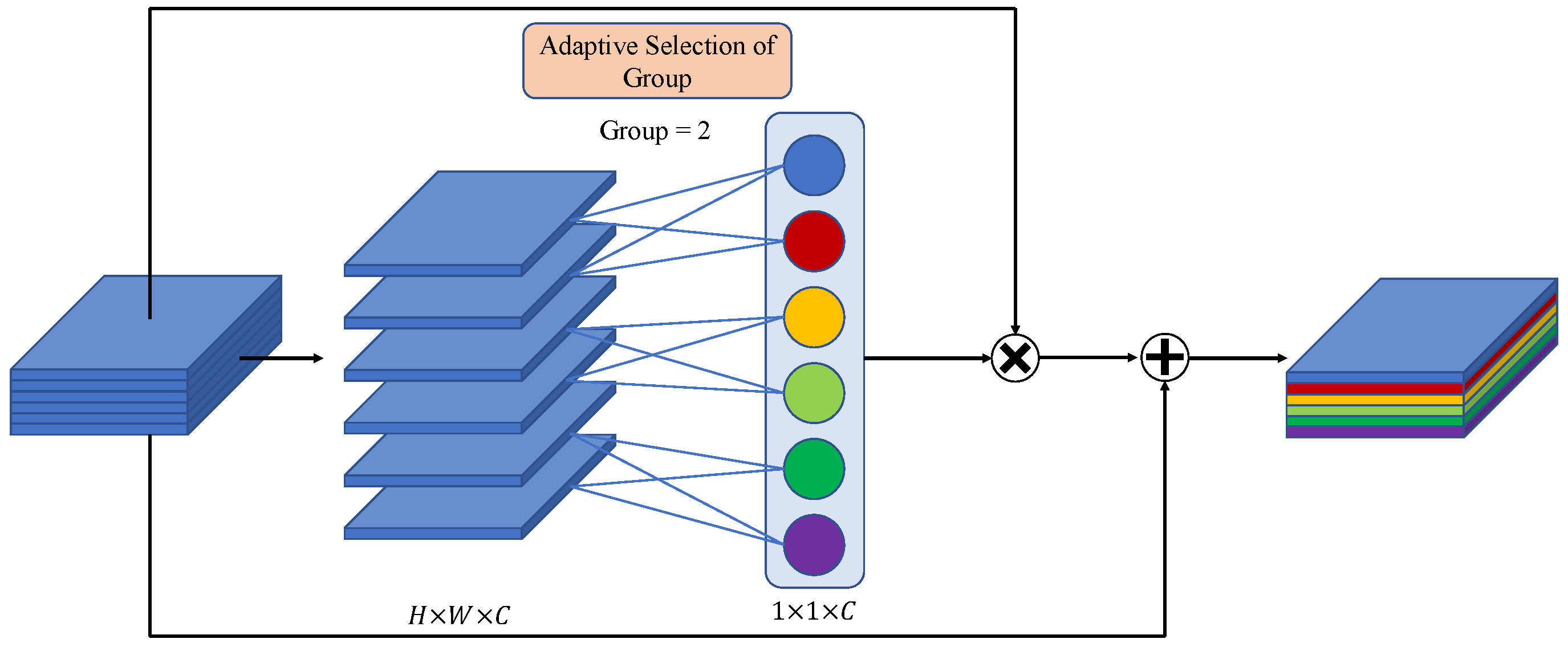
In our designed channel attention mechanism, the form of W in Equation (3) is matrix (5). In this equation, k represents the number of groups. When the value of k is larger, there will be more levels of features for communicating information across channels, and the number of parameters of the network will increase accordingly. In our experiments, we set k to 4. We chose a super-large convolution kernel as the convolution kernel of the grouped convolution, and the size of the convolution kernel we chose is ( H , W ) , which is the size of the input feature map. The advantage of taking the convolution kernel of the same size as the feature map is to obtain a larger receptive field. Our proposed structure can process each pixel independently, and the overall calculation will not have coupling effects due to the use of small convolution kernels. Therefore, the network can have a better target positioning capability.
In the LFCA module, the residual structure is also used, and the network structure is shown in Figure 6. We use a total of four such structures, which are connected after the output of the features by the CFP. After the feature map with shape ( H , W , C ) enters this module, the weights with shape ( 1 , 1 , C ) are generated by the grouping convolution layer. k in matrix (5) is represented by “Group” in the figure. The larger the value of this parameter is, the more channels will be crossed. Then the generated weights are multiplied by the feature and added to the feature to obtain the final output of this module. The calculation process of the LFCA module can be described as follows:
F = σ ( Y + G C ( Y ) )
where G C means group convolution layer, and Y is the set of features obtained from the previous process.

3.4. Auxiliary Branch

The content of SAR images can be divided into two parts, building area and non-building area (background area). In order to reduce the phenomenon of recognizing the objects in non-building areas as buildings in the process of segmentation, we designed the auxiliary branch. The input of the auxiliary branch is the third level of the feature obtained after the image is processed by the feature segmenter; that is, β 2 . The network structure adopted by the auxiliary branch is the classic FCN network. The calculation process of the auxiliary branch can be described as follows:
F = c o n v 2 ( c o n v 1 ( β 2 ) )
where c o n v 1 represents a 3 × 3 convolution. c o n v 2 represents anothor 3 × 3 convolution.

3.5. Loss Function

The final feature map obtained after processing with the semantic segmenter is F 1 . The final feature map obtained after processing with the auxiliary branch is F 2 . The generated features are then passed through a CLS layer to get the final predicted output. The calculation process can be described as follows:
P 1 = c o n v 1 ( F 1 ) P 2 = c o n v 3 ( F 2 )
where P 1 , P 2 represents the predicted output of the two segmenters, c o n v 1 represents a 3 × 3 convolution, the other parameters are i n _ c h a n n e l = 512 , o u t _ c h a n n e l = 4 . c o n v 3 represents a 3 × 3 convolution, and the other parameters are i n _ c h a n n e l = 512 , o u t _ c h a n n e l = 2 . In the training phase, our LRFFNet uses the standard cross-entropy loss as the loss function, and there is one in each of the semantic segmenter and auxiliary branches, which is defined as follows:
l o s s 1 ( P 1 , G 1 ) = 1 N k = 1 N [ G k 1 l o g ( P k 1 ) + ( 1 G K 1 ) l o g ( 1 P k 1 ) ] l o s s 2 ( P 2 , G 2 ) = 1 N k = 1 N [ G k 2 l o g ( P k 2 ) + ( 1 G K 2 ) l o g ( 1 P k 2 ) ]
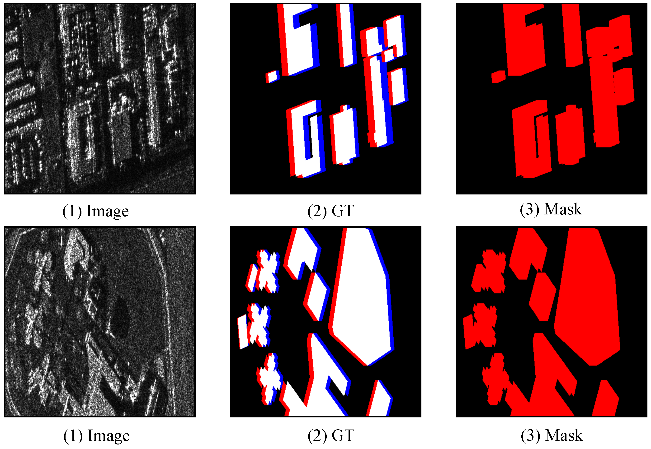
where G 1 denotes the ground-truth images, while G 2 denotes the mask images. Figure 7 shows the two types of images. The details of producing mask images can be seen in Section 4.3.3. k is the index of pixels, and N is the number of pixels in P 1 and P 2 . The total loss can be written as Equation (10), where α is set to 0.2 in our experiment.
l o s s = l o s s 1 + α l o s s 2

4. Experiments and Discussion

In this section, we conducted extensive experiments using the SARMV3D-BIS dataset to evaluate the performance of our proposed method. To achieve this goal, we compared our method with some SOTA methods and analyzed the results. The details of the experimental setup are in Section 4.1. The comparison experiments and analysis of our method and SOTA methods on the SARMV3D-BIS dataset are provided in Section 4.2. The ablation experiments and analysis of our model are presented in Section 4.3. The analysis of our method is provided in Section 4.4.

4.1. Experimental Settings

4.1.1. Dataset Description

To prove the effectiveness of our proposed method on SAR image semantic segmentation in building areas, the benchmark dataset we use is the SARMV3D-BIS dataset [65], produced by the Chinese Academy of Sciences team.
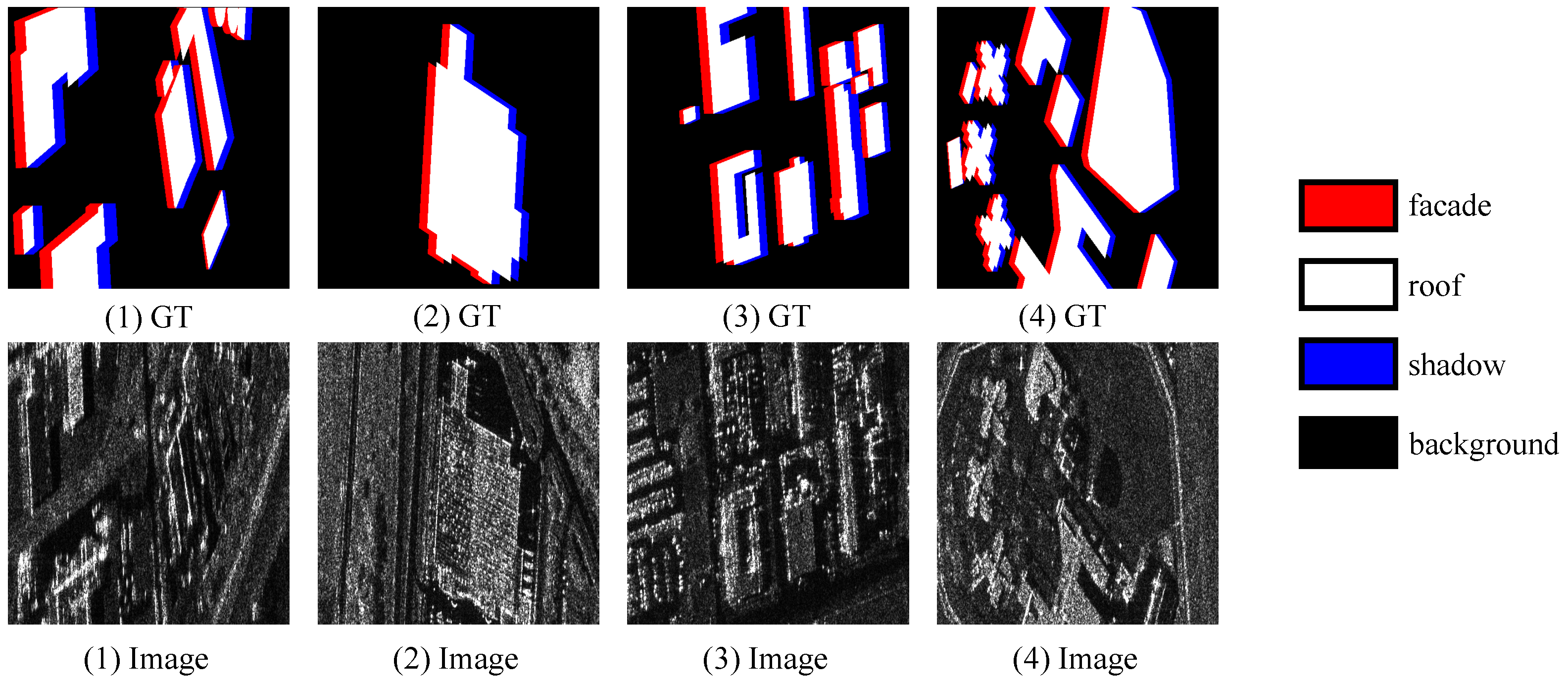
The original SAR images in the dataset come from the Omaha city area of the United States in the GF-3 beam stacking mode. According to the systematic process and method of labeling based on the 3D model simulation back projection proposed by the data production team, the SAR images are refined semantically. It contains the facade, roof, and shadow of each building.
Figure 8 shows a partial dataset, and each column is a data pair. The first row is the ground truth, where red represents the facade of the building, white represents the roof of the building, blue represents the shadow of the building, and black represents the background. The second row corresponds to the SAR image. The size of each image is 512 × 512 pixels. The dataset can be divided into training set, validation set, and test set. The training set contains 1280 image pairs, the validation set contains 369 image pairs, and the test set contains 369 image pairs.

4.1.2. Comparison Methods and Evaluation Metrics

To demonstrate the superiority of our method for segmentation tasks on SAR images in building areas, we compared the proposed LRFFNet with SOTA semantic segmentation methods, which are UNet [35], EncNet [36], ApcNet [37], EmaNet [38], DeepLabV3 [41], PspNet [43], DaNet [44], FPN [63], MP-ResNet [50], HR-SARNet [49], and MS-FCN [51].
To fairly compare with the SOTA methods on the SARMV3D-BIS dataset, we use the widely used evaluation metrics, including intersection over union ( I o U ) , mean intersection over union ( m I o U ) , Accuracy ( A c c ) , mean Accuracy ( m A c c ) , and all Accuracy ( a A c c ) .
The I o U is calculated as follows:
I o U i = G T i P r e d i G T i P r e d i
m I o U = i n I o U i
The A c c is calculated as follows:
A c c = T P + T N T P + F N + F P + F N
m A c c = i n A c c i
a A C C = N u m T r u e N u m
where i denotes the semantic categories and n is the number of classes. In particular, a A c c is calculated by dividing the number of all correctly classified pixels in the prediction map by the total number of pixels.

4.1.3. Implementation Details

Our network was tested on the following platforms, including AMD Ryzen 5 5600× CPU @3.7 GHz, NVIDIA RTX 3090 Ti GPU with CUDA version 11.6. In the experimental setting, we use random flip and random rotation data augmentation methods for the input image, and the probability is set to 0.5. The optimizer we use is the adamw optimizer, where l r is set to 0.0008, coefficients used for computing running averages of the gradient and its square betas are set to (0.9, 0.999), the weight decay coefficient is 0.05, the warmup and learning rate decay strategies are used at the same time, the warm-up interval is set to 300, the warmup ratio is set to 0.001, and the decay strategy uses the poly strategy. The batch size was set to 8, and the network was trained in 20,000 steps.

4.2. Comparative Experiments and Analysis

We followed the experimental setup in Section 4.1, and several groups of comparative experiments were carried out.
The SARMV3D-BIS dataset is a challenging task. SAR images already contain much useful information, such as the structure, texture, and occlusion relationship between the environment and the target. However, SAR images contain information about the microwave band and have a lower signal-to-noise ratio compared with optical images. Optical images can be distinguished well by the human eye, but interpreting SAR images requires professional knowledge. Therefore, it is more challenging to interpret SAR images. The segmentation of SAR images is more complicated. We made a statistic on the area of each category in the dataset. The proportions of the four categories (background, facade, roof, and shadow) in the dataset are 76.14%, 5.27%, 14.01%, and 4.57%. It can be seen that the background accounts for a large part of the dataset, and the building area accounts for less than 50%. In addition, the roof category in the building area accounts for a considerable part, but the facade and shadow only account for less than 6%, which are small objects. The unbalanced distribution of data categories is an important reason for why this dataset is challenging for performing semantic segmentation tasks.
We conduct experiments on the SARMV3D-BIS dataset using our method and some other SOTA methods, and most comparison methods are improved based on the encoder-decoder structure. For a more rigorous comparison, our experiments can be divided into three groups. In the first set of experiments, the comparison method entirely refers to the original paper, and most of them use the ResNet encoder. The experimental results are shown in Table 1. In the second set of experiments, the comparison method uses ConvNeXt as the encoder, which uses the same encoder as our proposed method. The purpose of setting up this set of experiments is to eliminate the effects of using the different encoders. The experimental results are shown in Table 2. In the third set of experiments, we compared our method with the advanced network specially designed for SAR image segmentation. In the three tables, the best experiment result is marked in red, and the following best experiment result is marked in blue.
As shown in Table 1, our proposed method outperforms other methods in various evaluation metrics. Specifically, the mIoU score of our LRFFNet is 8.16 % higher than the second-best method, DaNet. The mAcc score of our LRFFNet is 8.16 % higher than the second-best method, DeepLabV3. The aAcc score of our LRFFNet is 2.73 % higher than the second-best method, DaNet.
As shown in Table 2, compared with the SOTA method, our proposed method improves on most evaluation metrics. Specifically, the mIoU score of our LRFFNet is 3.09 % higher than the second-best method, DeepLabV3. In particular, the IoU scores of LRFFNet in background and roof increased by 0.38% and 2.82% compared to second place. Our method also achieves SOTA performance on the hard-to-segment semantic classes of “facade” and “shadow”. On the segmentation of “facade” objects, the IoU score of our LRFFNet is 4.94% higher than the second-best method, DeepLabV3. On the segmentation of “shadow” objects, the IoU score of our LRFFNet is 2.68% higher than the second-best method, DeepLabV3. The mAcc score of our LRFFNet is 2.76 % higher than the second-best method, DeeplabV3. In particular, on the segmentation of “facade” objects, the Acc score of our LRFFNet is 5.53 % higher than the second-best method, DeeplabV3. On the segmentation of “shadow” objects, the Acc score of our LRFFNet is 5.01 % higher than the second-best method, PspNet.
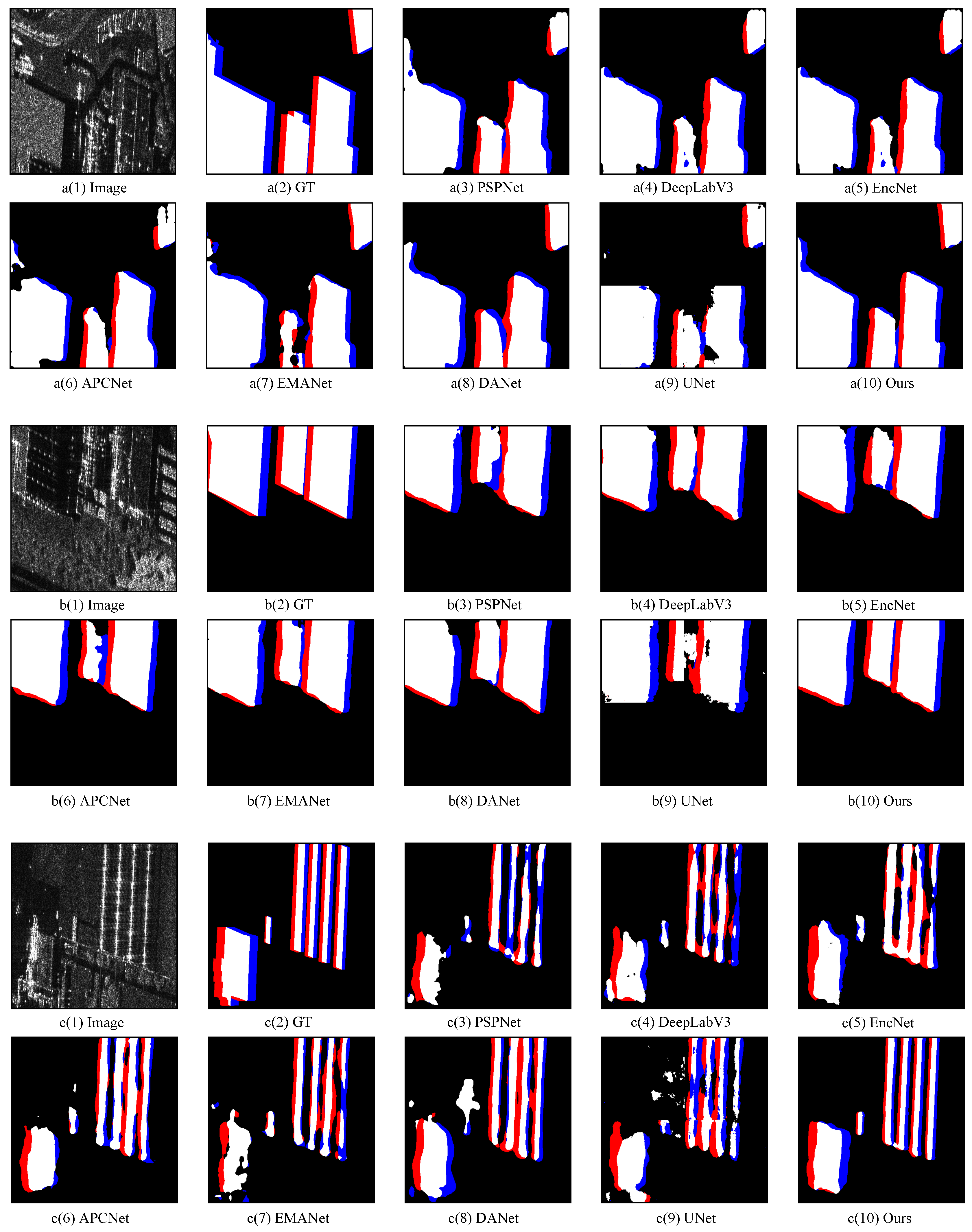
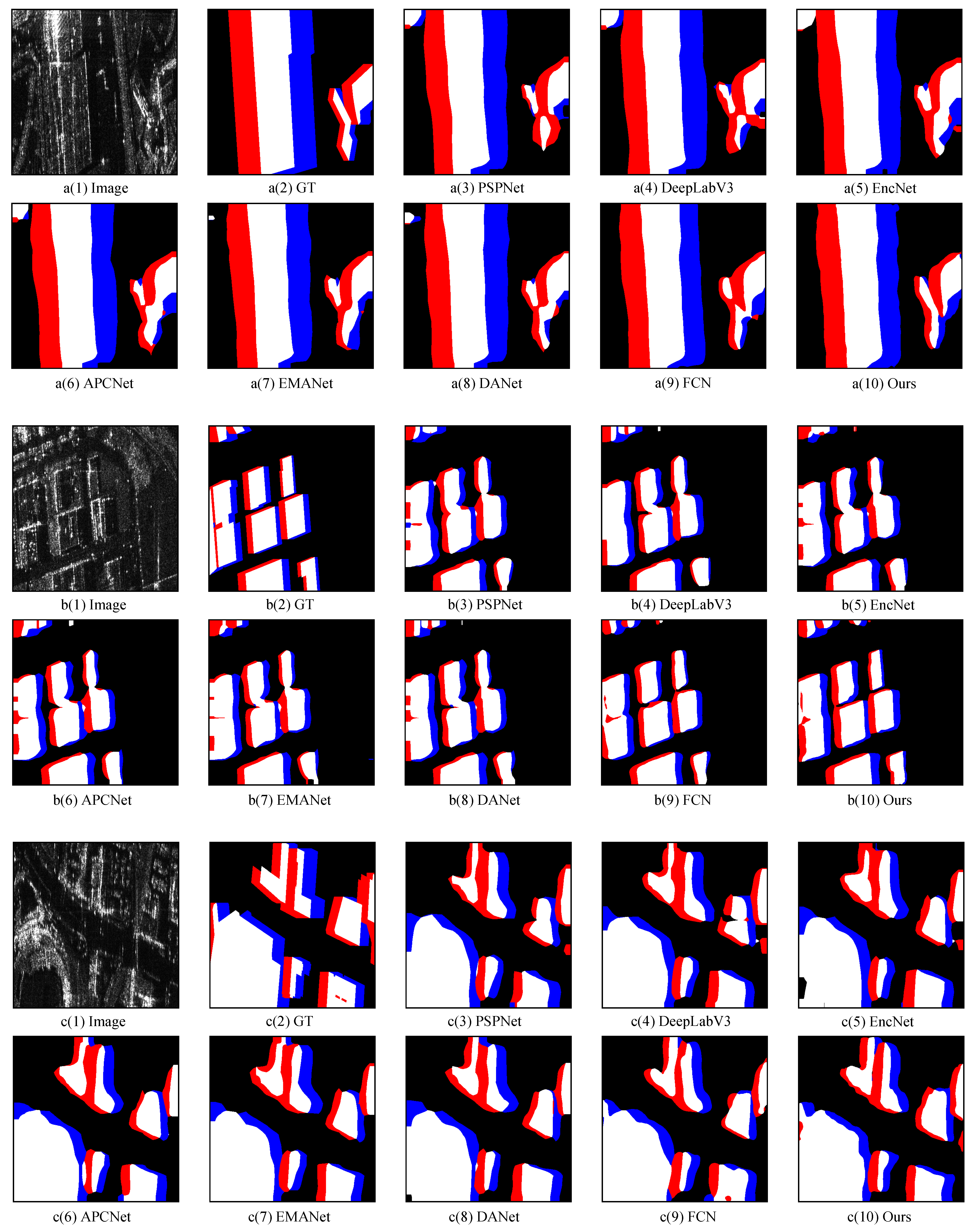
In addition, another series of comparative experiments was carried out between our method and methods designed for SAR image segmentation. The compared methods include MP-ResNet, HR-SARNet, and MS-FCN. The experimental results are shown in Table 3. As can be seen, our proposed method achieves improvements in all evaluation metrics. To intuitively demonstrate the superiority of our proposed LRFFNet in the semantic segmentation of SAR images in building areas, we performed visual comparison experiments and produced a comparison result graph. The visualization results are shown in Figure 9 and Figure 10. Every two rows in the figure are a set of comparative experiments, including the original image to be classified, the ground truth, and the classification result predicted by each method. Among them, the last block is the prediction result of our LRFFNet. Our proposed method has good segmentation accuracy whether in the larger category, such as background and roof, or in the smaller category, such as facade and shadow. Compared with other methods, the semantic segmentation results obtained by our method are closer to the ground-truth images in visual effect.

4.3. Ablation Experiments

In this subsection, we evaluated the effectiveness of two key modules of our proposed method, the cascade feature pyramid module (CFP) and the large receptive field channel attention module (LFCA). At the same time, we evaluated the effectiveness of the auxiliary branch.

4.3.1. Effect of Cascade Feature Pyramid Module

We first set up a basic experiment ( c o n v N + F P N ) in which we use ConvNeXt as the feature extractor and FPN as the decoder. After that, we trained the ( c o n v N + C F P ) network and the ( c o n v N + C C F P ) network. These three sets of comparative experiments prove the effectiveness of our proposed feature fusion module. At the same time, it is proven that CFP can be used as a basic unit, and the network structure obtained by concatenating CFP has better segmentation ability.
The comparison results of the three experiments can be seen in Table 4. Comparing the results of the experiment ( c o n v N + F P N ) and the experiment ( c o n v N + C F P ) , after using our proposed CFP, the evaluation index m I o U increased by 1.43 % , m A c c increased by 1.21 % , and a A c c increased by 0.38 % . Comparing the results of experiment ( c o n v N + C F P ) and experiment ( c o n v N + C C F P ) , the evaluation index m I o U increased by 0.66 % , m A c c increased by 0.61 % , and a A c c increased by 0.12 % . This performance benefits from our redesigned feature fusion path and redesigned feature fusion method. It proved that the CFP layer could be regarded as a network unit, which can be flexibly combined and used in series to expand the network capacity and improve the effectiveness of the network.

4.3.2. Effect of the Large Receptive Field Channel Attention Module

We first set up a basic experiment ( c o n v N + C F P ) in which we use ConvNeXt as the feature extractor and FPN as the decoder; then we trained the ( c o n v N + C C F P + L F C A ) model to evaluate the effectiveness of our proposed LFCA. Table 5 shows the result of the two experiments. It shows that after adding the LFCA model, the evaluation index m I o U increased by 1.36%, the I o U of the facade increased by 2.19%, and the I o U of the shadow increased by 2.19%. It can be seen that due to the addition of the attention mechanism we proposed, the classification effect on small objects has been improved. At the same time, the segmentation effect in other categories has also been improved. The I o U of the background has increased by 0.36%, and the I o U of the roof has increased by 1.85%. In the ( c o n v + C C F P + L F C A ) model, the m A c c evaluation index increased by 1.33%, the A c c of facade increased by 2.54%, the A c c of shadow increased by 0.7%, and the A c c of roof increased by 2.07%. The LFCA model can distinguish between the importance of channels, assign greater weight to channels that contain helpful information, and assign small weights to channels with less content. LFCA helps the network pay more attention to the information-rich channels, highlight the areas of significant interest, and improve the network training effect.
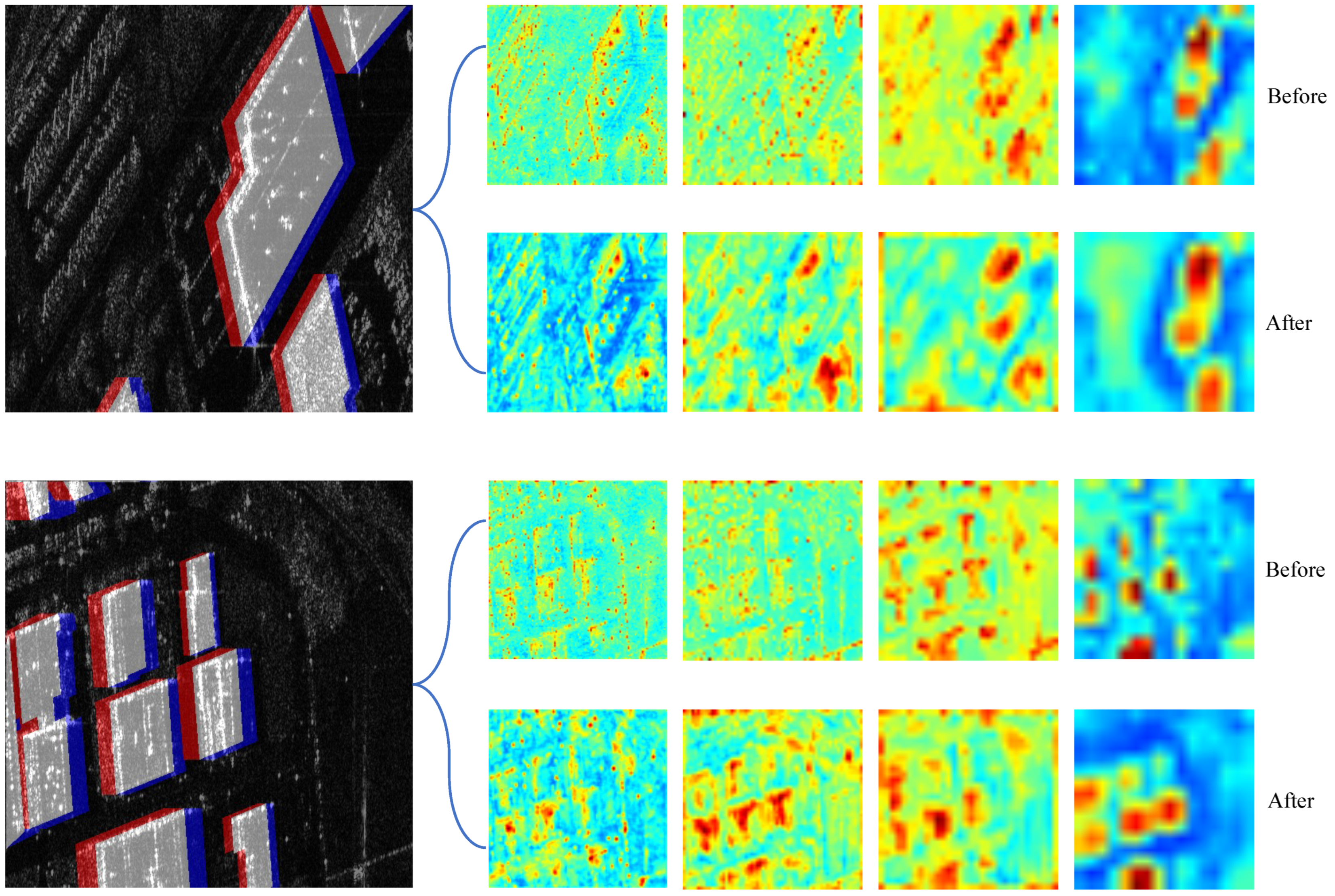
To more intuitively understand the role of the LFCA layer, we performed visual processing of the features before and after the LFCA layer. The features before going through the LFCA layer are expressed as ( β 0 , β 1 , β 2 , β 3 ) , and the features after going through the LFCA layer are expressed as ( β 0 , β 1 , β 2 , β 3 ) . The visualization result shown in Figure 11 contains two examples. In order to make the SAR image and the label have a more intuitive correspondence, we fused the original SAR image and the GT image with 50 % each to generate the “image”. “Before” stands for the visualization result before the LFCA structure processes the feature, and “After” stands for the visualization result after the LFCA structure processes the feature. The warmer color temperature in the picture represents the more significant value in the feature, representing the area the network pays more attention to. As can be seen in the figure, the feature map after LFCA processing highlights the area where the target is located. The target and the background areas are more clearly distinguished.

4.3.3. Effect of the Auxiliary Branch

The dataset we use has the following characteristics: the three categories of roofs, facades, and shadows appear simultaneously and are closely connected. Every building contains all three parts simultaneously. Therefore, we can divide the images into two categories: building and non-building areas. In some segmentation results, the ground objects in the non-building areas are identified as buildings. To reduce the occurrence of such phenomena, we design an auxiliary branch.
The auxiliary branch is to add a segmentation branch to the original network. In our setting, we put this branch after the features extracted by stage 2, and the network structure is a classic FCN network. We want to strengthen the supervision of features and optimize the quality of prediction results by adding an auxiliary branch. The following experiments confirm that the auxiliary branch can achieve such an effect.
We first processed the original GT image and unified the three categories of roof, shadow, and facade as one category. The generated mask image only contains two categories: building and background. The dataset after processing is shown in Figure 7. Each row is a set of data, including the original image to be segmented, the ground truth, and the mask image. The image predicted by the auxiliary branch is compared with the mask image, then the loss is calculated, and then back-propagation is performed to update the network parameters. The images predicted in the auxiliary branch and the mask images are used for loss calculation. As mentioned in Section 3.5, our network contains two loss functions: AUX loss and SEG loss. In order to select the appropriate loss ratio, we carried out several experiments and selected three representative groups of results for display. The experimental results are shown in Table 6, where α comes from Equation (10) and represents the ratio between the two losses. It can be seen from the data in the table that when we set the ratio of aux loss and seg loss to 2:1, each index of the network has decreased compared with the evaluation metrics in Table 5. Specifically, the evaluation index m I o U decreased by 0.61 % , m A c c increased by 0.12 % , and A c c increased by 0.23 % . When we set this ratio to 1:1 and 0.2:1, the network has a small improvement in each index, and when the ratio is 0.2:1, the score on each index is even higher. Specifically, the evaluation index m I o U increased by 0.30 % , and m A c c increased by 0.64 % . Therefore, we set the ratio of the loss function as 0.2:1 in LRFFNet.
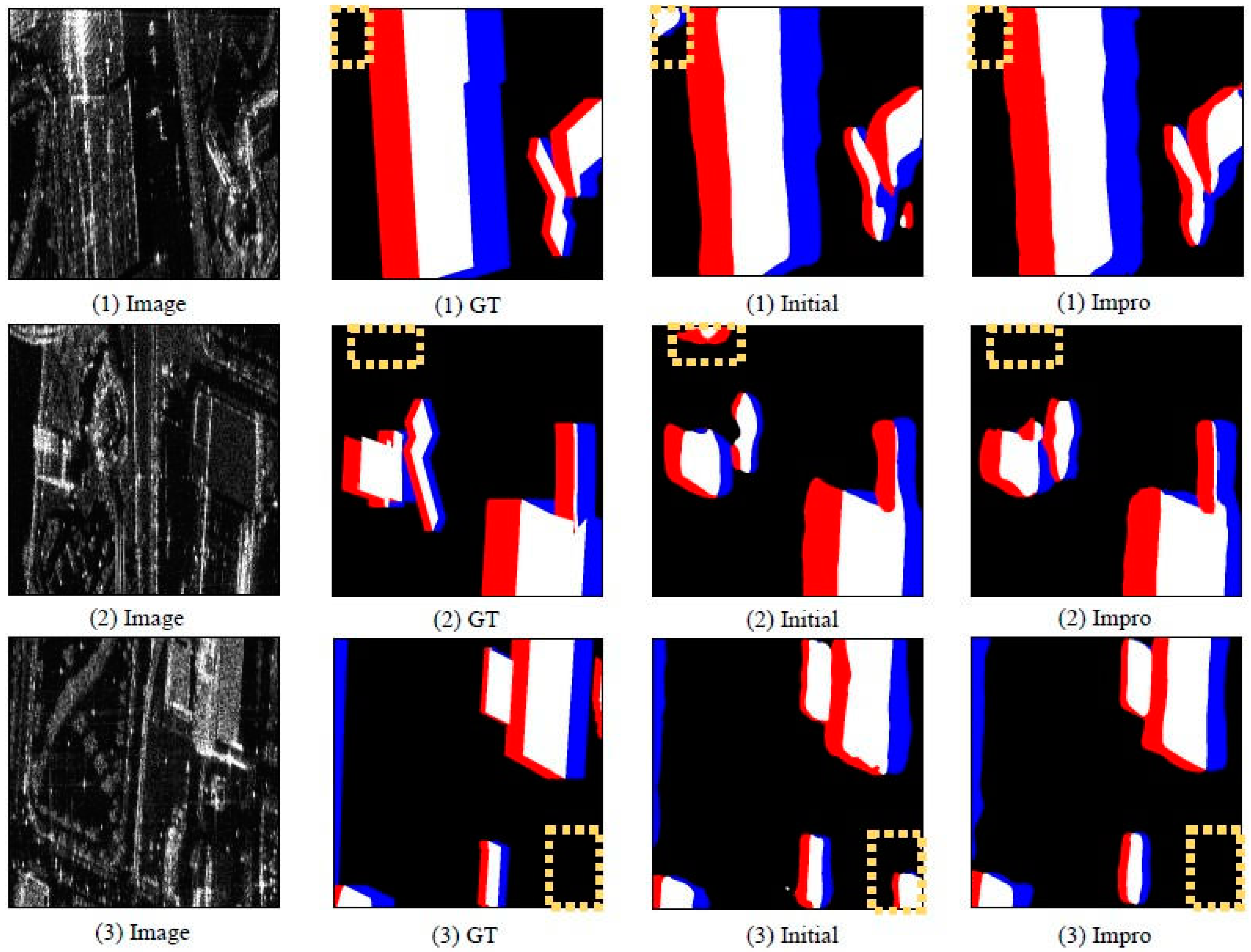
The experimental results are shown in Figure 12. Each column is a set of data. “Image” stands for the original input image, “GT” stands for ground truth, “Initia” stands for the prediction result graph before adding auxiliary branches, and “Impro” stands for the prediction result graph after adding an auxiliary branch. We marked the parts of the image that needed special attention with a yellow dotted box. Comparing “Initial” and “Impro” images, it can be seen from the experimental results that the phenomenon of separate color blocks outside the mask area is reduced. Due to the use of the mask images, the network can focus more on segmentation within the building areas and reduce the misclassification of pixels outside the building areas as buildings. The segmentation results are closer to the ground truth.

4.4. Analysis of Methods

We compared the proposed method with the SOTA methods on the SARMV3D-BIS dataset and improved the evaluation metrics of m I o U , a A c c , and m A c c . According to the results graph, the semantic segmentation results obtained using LRFFNet are closer to the ground truth in visual perception. Later, in the ablation experiment, we used the control variable method to perform a validation experiment on each module we proposed, namely, CFP, LFCA, and the auxiliary branch. The multi-path feature fusion structure and convolution feature fusion method are adopted in the CFP structure. Grouped convolution is used in the LFCA structure to extract the channel weight value. By using the large convolution kernel, different weights are given to the channels to emphasize the differences between channels. The FCN structure is adopted in the auxiliary branch. It is added to the network to reduce the occurrence of identifying ground objects in non-building areas as buildings. The results of ablation experiments show that the various modules we proposed are very effective for the SAR image semantic segmentation task.

5. Conclusions

In this paper, we propose a new framework for semantic segmentation of the synthetic aperture radar (SAR) images in building areas named large receptive field feature fusion network (LRFFNet), which contains four components, namely, the feature extractor, the cascade feature pyramid module (CFP), the large receptive field channel attention module (LFCA), and the auxiliary branch. The dataset we use is SARMV3D-BIS. The semantic segmentation task on SAR images differs from optical images. The boundary information between objects is not apparent in the SAR images, so it is more challenging to extract semantic information. Our proposed network can fully fuse the features extracted by the feature extractor through a multi-path connection structure and enable sufficient information exchange between different levels. At the same time, our proposed network can also distinguish the importance of different channels in each feature level, highlight channels with more information, and reduce the importance of channels with less information. In addition, we observed ground objects in non-building areas being identified as buildings in some segmentation results. Therefore, we design an auxiliary branch in our network to facilitate the segmentation of our network in the building area through the supervision of the intermediate layer and improve the score of evaluation metrics. Semantic segmentation on SAR images is still developing, and many aspects can be improved, studied, and explored. We hope this research can inspire more researchers in this area and deploy practical applications.

Author Contributions

B.P. and W.Z. proposed the original idea. B.P. performed the experiments and wrote the manuscript. W.Z. and Y.H. reviewed and edited the manuscript. B.P., W.Z., Q.L. and Q.C. contributed to the direction, content, and revised the manuscript. All authors have read and agreed to the published version of the manuscript.

Funding

This research was supported by the National Natural Science Foundation of China under grant number 61860206013.

Data Availability Statement

The SARMV3D-BIS dataset is openly available in Journal of Radars at https://radars.ac.cn/web/data/getData?dataType=SARMV3D (accessed on 4 December 2022).

Conflicts of Interest

The authors declare no conflict of interest.

References

  1. Curlander, J.C.; McDonough, R.N. Synthetic Aperture Radar; Wiley: New York, NY, USA, 1991; Volume 11. [Google Scholar]
  2. Chen, F.; Lasaponara, R.; Masini, N. An overview of satellite synthetic aperture radar remote sensing in archaeology: From site detection to monitoring. J. Cult. Herit. 2017, 23, 5–11. [Google Scholar] [CrossRef]
  3. Moreira, A.; Prats-Iraola, P.; Younis, M.; Krieger, G.; Hajnsek, I.; Papathanassiou, K.P. A tutorial on synthetic aperture radar. IEEE Geosci. Remote Sens. Mag. 2013, 1, 6–43. [Google Scholar] [CrossRef] [Green Version]
  4. Cumming, I.G.; Wong, F.H. Digital processing of synthetic aperture radar data. Artech House 2005, 1, 108–110. [Google Scholar]
  5. Joyce, K.E.; Samsonov, S.; Levick, S.R.; Engelbrecht, J.; Belliss, S. Mapping and monitoring geological hazards using optical, LiDAR, and synthetic aperture RADAR image data. Nat. Hazards 2014, 73, 137–163. [Google Scholar] [CrossRef]
  6. Chen, J.; Qiu, X.; Ding, C.; Wu, Y. CVCMFF Net: Complex-valued convolutional and multifeature fusion network for building semantic segmentation of InSAR images. IEEE Trans. Geosci. Remote Sens. 2021, 60, 1–14. [Google Scholar] [CrossRef]
  7. Mangai, U.G.; Samanta, S.; Das, S.; Chowdhury, P.R.; Varghese, K.; Kalra, M. A hierarchical multi-classifier framework for landform segmentation using multi-spectral satellite images-a case study over the indian subcontinent. In Proceedings of the 2010 Fourth Pacific-Rim Symposium on Image and Video Technology, Singapore, 14–17 November 2010; pp. 306–313. [Google Scholar]
  8. Yu, Q.; Clausi, D.A. IRGS: Image segmentation using edge penalties and region growing. IEEE Trans. Pattern Anal. Mach. Intell. 2008, 30, 2126–2139. [Google Scholar]
  9. Jogin, M.; Madhulika, M.; Divya, G.; Meghana, R.; Apoorva, S. Feature extraction using convolution neural networks (CNN) and deep learning. In Proceedings of the 2018 3rd IEEE International Conference on Recent Trends in Electronics, Information & Communication Technology (RTEICT), Bengaluru, Karnataka, 18–19 May 2018; pp. 2319–2323. [Google Scholar]
  10. Yuan, X.; Shi, J.; Gu, L. A review of deep learning methods for semantic segmentation of remote sensing imagery. Expert Syst. Appl. 2021, 169, 114417. [Google Scholar] [CrossRef]
  11. Guo, Y.; Liu, Y.; Georgiou, T.; Lew, M.S. A review of semantic segmentation using deep neural networks. Int. J. Multimed. Inf. Retr. 2018, 7, 87–93. [Google Scholar] [CrossRef] [Green Version]
  12. Orfanidis, G.; Ioannidis, K.; Avgerinakis, K.; Vrochidis, S.; Kompatsiaris, I. A deep neural network for oil spill semantic segmentation in Sar images. In Proceedings of the 2018 25th IEEE International Conference on Image Processing (ICIP), Athens, Greece, 7–10 October 2018; pp. 3773–3777. [Google Scholar]
  13. Tupin, F. Extraction of 3D information using overlay detection on SAR images. In Proceedings of the 2003 2nd GRSS/ISPRS Joint Workshop on Remote Sensing and Data Fusion over Urban Areas, Berlin, Geramny, 22–23 May 2003; pp. 72–76. [Google Scholar]
  14. Ding, B.; Wen, G.; Ma, C.; Yang, X. An efficient and robust framework for SAR target recognition by hierarchically fusing global and local features. IEEE Trans. Image Process. 2018, 27, 5983–5995. [Google Scholar] [CrossRef]
  15. Ma, A.; Wang, J.; Zhong, Y.; Zheng, Z. Factseg: Foreground activation-driven small object semantic segmentation in large-scale remote sensing imagery. IEEE Trans. Geosci. Remote Sens. 2021, 60, 1–16. [Google Scholar] [CrossRef]
  16. Zhang, M.; Li, Z.; Tian, B.; Zhou, J.; Tang, P. The backscattering characteristics of wetland vegetation and water-level changes detection using multi-mode SAR: A case study. Int. J. Appl. Earth Obs. Geoinf. 2016, 45, 1–13. [Google Scholar] [CrossRef]
  17. Garcia-Garcia, A.; Orts-Escolano, S.; Oprea, S.; Villena-Martinez, V.; Garcia-Rodriguez, J. A review on deep learning techniques applied to semantic segmentation. arXiv 2017, arXiv:1704.06857. [Google Scholar]
  18. Sun, Z.; Geng, H.; Lu, Z.; Scherer, R.; Woźniak, M. Review of road segmentation for SAR images. Remote Sens. 2021, 13, 1011. [Google Scholar] [CrossRef]
  19. Cohen, A.; Rivlin, E.; Shimshoni, I.; Sabo, E. Memory based active contour algorithm using pixel-level classified images for colon crypt segmentation. Comput. Med. Imaging Graph. 2015, 43, 150–164. [Google Scholar] [CrossRef] [PubMed]
  20. Dalal, N.; Triggs, B. Histograms of oriented gradients for human detection. In Proceedings of the 2005 IEEE Computer Society Conference on Computer Vision and Pattern Recognition (CVPR’05), San Diego, CA, USA, 20–25 June 2005; Volume 1, pp. 886–893. [Google Scholar]
  21. Lowe, D.G. Distinctive image features from scale-invariant keypoints. Int. J. Comput. Vis. 2004, 60, 91–110. [Google Scholar] [CrossRef]
  22. Csurka, G.; Dance, C.; Fan, L.; Willamowski, J.; Bray, C. Visual categorization with bags of keypoints. In Proceedings of the Workshop on Statistical Learning in Computer Vision, Prague, Czech Republic, 11–14 May 2004; Volume 1, pp. 1–2. [Google Scholar]
  23. Chen, C.W.; Luo, J.; Parker, K.J. Image segmentation via adaptive K-mean clustering and knowledge-based morphological operations with biomedical applications. IEEE Trans. Image Process. 1998, 7, 1673–1683. [Google Scholar] [CrossRef] [Green Version]
  24. Carreira, J.; Sminchisescu, C. Constrained parametric min-cuts for automatic object segmentation. In Proceedings of the 2010 IEEE Computer Society Conference on Computer Vision and Pattern Recognition, San Francisco, CA, USA, 13–18 June 2010; pp. 3241–3248. [Google Scholar]
  25. Ma, F.; Xiang, D.; Yang, K.; Yin, Q.; Zhang, F. Weakly Supervised Deep Soft Clustering for Flood Identification in SAR Images. IEEE Geosci. Remote Sens. Lett. 2022, 19, 1–5. [Google Scholar] [CrossRef]
  26. Du, B.; Ru, L.; Wu, C.; Zhang, L. Unsupervised deep slow feature analysis for change detection in multi-temporal remote sensing images. IEEE Trans. Geosci. Remote Sens. 2019, 57, 9976–9992. [Google Scholar] [CrossRef] [Green Version]
  27. Huang, S.; Zhang, H.; Pižurica, A. Subspace clustering for hyperspectral images via dictionary learning with adaptive regularization. IEEE Trans. Geosci. Remote Sens. 2021, 60, 1–17. [Google Scholar] [CrossRef]
  28. Kass, M.; Witkin, A.; Terzopoulos, D. Snakes: Active contour models. Int. J. Comput. Vis. 1988, 1, 321–331. [Google Scholar] [CrossRef]
  29. Roerdink, J.B.; Meijster, A. The watershed transform: Definitions, algorithms and parallelization strategies. Fundam. Inform. 2000, 41, 187–228. [Google Scholar] [CrossRef] [Green Version]
  30. Ho, T.K. Random decision forests. In Proceedings of the 3rd International Conference on Document Analysis and Recognition, Montreal, QC, Canada, 14–16 August 1995; Volume 1, pp. 278–282. [Google Scholar]
  31. Burges, C.J. A tutorial on support vector machines for pattern recognition. Data Min. Knowl. Discov. 1998, 2, 121–167. [Google Scholar] [CrossRef]
  32. Blake, A.; Kohli, P.; Rother, C. Markov Random Fields for Vision and Image Processing; MIT Press: Cambridge, MA, USA, 2011. [Google Scholar]
  33. Sutton, C.; McCallum, A. An introduction to conditional random fields. Found. Trends Mach. Learn. 2012, 4, 267–373. [Google Scholar] [CrossRef]
  34. Long, J.; Shelhamer, E.; Darrell, T. Fully convolutional networks for semantic segmentation. In Proceedings of the IEEE Conference on Computer Vision and Pattern Recognition, Boston, MA, USA, 7–12 June 2015; pp. 3431–3440. [Google Scholar]
  35. Ronneberger, O.; Fischer, P.; Brox, T. U-net: Convolutional networks for biomedical image segmentation. In Proceedings of the International Conference on Medical Image Computing and Computer-Assisted Intervention, Singapore, 18–22 September 2015; pp. 234–241. [Google Scholar]
  36. Zhang, H.; Dana, K.; Shi, J.; Zhang, Z.; Wang, X.; Tyagi, A.; Agrawal, A. Context encoding for semantic segmentation. In Proceedings of the IEEE conference on Computer Vision and Pattern Recognition, Salt Lake City, UT, USA, 18–23 June 2018; pp. 7151–7160. [Google Scholar]
  37. He, J.; Deng, Z.; Zhou, L.; Wang, Y.; Qiao, Y. Adaptive pyramid context network for semantic segmentation. In Proceedings of the IEEE/CVF Conference on Computer Vision and Pattern Recognition, Long Beach, CA, USA, 15–20 June 2019; pp. 7519–7528. [Google Scholar]
  38. Li, X.; Zhong, Z.; Wu, J.; Yang, Y.; Lin, Z.; Liu, H. Expectation-maximization attention networks for semantic segmentation. In Proceedings of the IEEE/CVF International Conference on Computer Vision, Seoul, Republic of Korea, 27 October–2 November 2019; pp. 9167–9176. [Google Scholar]
  39. Chen, L.C.; Papandreou, G.; Kokkinos, I.; Murphy, K.; Yuille, A.L. Semantic image segmentation with deep convolutional nets and fully connected crfs. arXiv 2014, arXiv:1412.7062. [Google Scholar]
  40. Chen, L.C.; Papandreou, G.; Kokkinos, I.; Murphy, K.; Yuille, A.L. Deeplab: Semantic image segmentation with deep convolutional nets, atrous convolution, and fully connected crfs. IEEE Trans. Pattern Anal. Mach. Intell. 2017, 40, 834–848. [Google Scholar] [CrossRef] [Green Version]
  41. Chen, L.C.; Papandreou, G.; Schroff, F.; Adam, H. Rethinking atrous convolution for semantic image segmentation. arXiv 2017, arXiv:1706.05587. [Google Scholar]
  42. Chen, L.C.; Zhu, Y.; Papandreou, G.; Schroff, F.; Adam, H. Encoder-decoder with atrous separable convolution for semantic image segmentation. In Proceedings of the European Conference on Computer Vision (ECCV), Munich, Germany, 8–14 September 2018; pp. 801–818. [Google Scholar]
  43. Zhao, H.; Shi, J.; Qi, X.; Wang, X.; Jia, J. Pyramid scene parsing network. In Proceedings of the IEEE Conference on Computer Vision and Pattern Recognition, Honolulu, HI, USA, 21–26 July 2017; pp. 2881–2890. [Google Scholar]
  44. Fu, J.; Liu, J.; Tian, H.; Li, Y.; Bao, Y.; Fang, Z.; Lu, H. Dual attention network for scene segmentation. In Proceedings of the IEEE/CVF Conference on Computer Vision and Pattern Recognition, Long Beach, CA, USA, 16–20 June 2019; pp. 3146–3154. [Google Scholar]
  45. Huang, Z.; Wang, X.; Huang, L.; Huang, C.; Wei, Y.; Liu, W. Ccnet: Criss-cross attention for semantic segmentation. In Proceedings of the IEEE/CVF International Conference on Computer Vision, Seoul, Republic of Korea, 27 October–2 November 2019; pp. 603–612. [Google Scholar]
  46. Wu, T.; Tang, S.; Zhang, R.; Cao, J.; Zhang, Y. Cgnet: A light-weight context guided network for semantic segmentation. IEEE Trans. Image Process. 2020, 30, 1169–1179. [Google Scholar] [CrossRef]
  47. Yu, C.; Wang, J.; Peng, C.; Gao, C.; Yu, G.; Sang, N. Bisenet: Bilateral segmentation network for real-time semantic segmentation. In Proceedings of the European Conference on Computer Vision (ECCV), Munich, Germany, 8–14 September 2018; pp. 325–341. [Google Scholar]
  48. Shaban, M.; Salim, R.; Abu Khalifeh, H.; Khelifi, A.; Shalaby, A.; El-Mashad, S.; Mahmoud, A.; Ghazal, M.; El-Baz, A. A deep-learning framework for the detection of oil spills from SAR data. Sensors 2021, 21, 2351. [Google Scholar] [CrossRef]
  49. Wang, X.; Cavigelli, L.; Eggimann, M.; Magno, M.; Benini, L. HR-SAR-Net: A deep neural network for urban scene segmentation from high-resolution SAR data. In Proceedings of the 2020 IEEE Sensors Applications Symposium (SAS), Kuala Lumpur, Malaysia, 9–11 March 2020; pp. 1–6. [Google Scholar]
  50. Ding, L.; Zheng, K.; Lin, D.; Chen, Y.; Liu, B.; Li, J.; Bruzzone, L. MP-ResNet: Multipath residual network for the semantic segmentation of high-resolution PolSAR images. IEEE Geosci. Remote Sens. Lett. 2021, 19, 1–5. [Google Scholar] [CrossRef]
  51. Wu, W.; Li, H.; Li, X.; Guo, H.; Zhang, L. PolSAR image semantic segmentation based on deep transfer learning—Realizing smooth classification with small training sets. IEEE Geosci. Remote Sens. Lett. 2019, 16, 977–981. [Google Scholar] [CrossRef]
  52. Yue, Z.; Gao, F.; Xiong, Q.; Wang, J.; Hussain, A.; Zhou, H. A novel attention fully convolutional network method for synthetic aperture radar image segmentation. IEEE J. Sel. Top. Appl. Earth Obs. Remote Sens. 2020, 13, 4585–4598. [Google Scholar] [CrossRef]
  53. He, W.; Song, H.; Yao, Y.; Jia, H. Mapping of Urban Areas from SAR Images via Semantic Segmentation. In Proceedings of the IGARSS 2020–2020 IEEE International Geoscience and Remote Sensing Symposium, Waikoloa, HI, USA, 26 September–2 October 2020; pp. 1440–1443. [Google Scholar]
  54. Cha, K.; Seo, J.; Choi, Y. Contrastive Multiview Coding with Electro-Optics for SAR Semantic Segmentation. IEEE Geosci. Remote Sens. Lett. 2021, 19, 1–5. [Google Scholar] [CrossRef]
  55. Davari, A.; Islam, S.; Seehaus, T.; Hartmann, A.; Braun, M.; Maier, A.; Christlein, V. On Mathews correlation coefficient and improved distance map loss for automatic glacier calving front segmentation in SAR imagery. IEEE Trans. Geosci. Remote Sens. 2021, 60, 1–12. [Google Scholar] [CrossRef]
  56. Bi, H.; Xu, L.; Cao, X.; Xue, Y.; Xu, Z. Polarimetric SAR image semantic segmentation with 3D discrete wavelet transform and Markov random field. IEEE Trans. Image Process. 2020, 29, 6601–6614. [Google Scholar] [CrossRef]
  57. Liu, Z.; Mao, H.; Wu, C.Y.; Feichtenhofer, C.; Darrell, T.; Xie, S. A convnet for the 2020s. In Proceedings of the IEEE/CVF Conference on Computer Vision and Pattern Recognition, New Orleans, LA, USA, 19–20 June 2022; pp. 11976–11986. [Google Scholar]
  58. He, K.; Zhang, X.; Ren, S.; Sun, J. Deep residual learning for image recognition. In Proceedings of the IEEE Conference on Computer Vision and Pattern Recognition, Las Vegas, NV, USA, 27–30 June 2016; pp. 770–778. [Google Scholar]
  59. Glorot, X.; Bordes, A.; Bengio, Y. Deep sparse rectifier neural networks. In Proceedings of the Fourteenth International Conference on Artificial Intelligence and Statistics. JMLR Workshop and Conference Proceedings, Lauderdale, FL, USA, 11–13 April 2011; pp. 315–323. [Google Scholar]
  60. Hendrycks, D.; Gimpel, K. Gaussian error linear units (gelus). arXiv 2016, arXiv:1606.08415. [Google Scholar]
  61. Ba, J.L.; Kiros, J.R.; Hinton, G.E. Layer normalization. arXiv 2016, arXiv:1607.06450. [Google Scholar]
  62. Ioffe, S.; Szegedy, C. Batch normalization: Accelerating deep network training by reducing internal covariate shift. In Proceedings of the International Conference on Machine Learning, Lille, France, 6–11 July 2015; pp. 448–456. [Google Scholar]
  63. Lin, T.Y.; Dollár, P.; Girshick, R.; He, K.; Hariharan, B.; Belongie, S. Feature pyramid networks for object detection. In Proceedings of the IEEE Conference on Computer Vision and Pattern Recognition, Honolulu, HI, USA, 21–26 July 2017; pp. 2117–2125. [Google Scholar]
  64. Hu, J.; Shen, L.; Sun, G. Squeeze-and-excitation networks. In Proceedings of the IEEE Conference on Computer Vision and Pattern Recognition, Salt Lake City, UT, USA, 18–23 June 2018; pp. 7132–7141. [Google Scholar]
  65. Luo, Y.; Qiu, X.; Peng, L.; Wang, W.; Lin, B.; Ding, C. A novel solution for stereo three-dimensional localization combined with geometric semantic constraints based on spaceborne SAR data. ISPRS J. Photogramm. Remote Sens. 2022, 192, 161–174. [Google Scholar] [CrossRef]
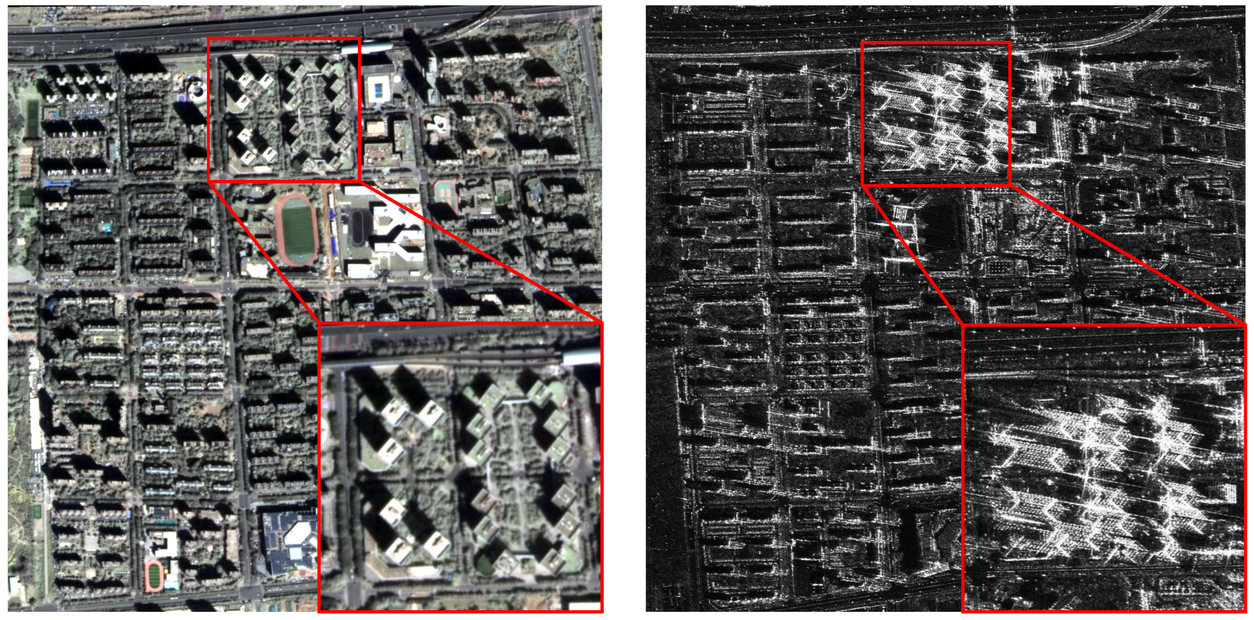
Figure 1. The comparison of an optical remote sensing image and a SAR image in the same area. The left image is the optical remote sensing image, the right image is the SAR image, and the high-rise building area is enlarged.
Remotesensing 14 06291 g001
Figure 2. Overall architecture.
Remotesensing 14 06291 g002
Figure 3. Feature extractor structure.
Remotesensing 14 06291 g003
Figure 4. Structure of the feature pyramid model (FPN).
Remotesensing 14 06291 g004
Figure 5. Structure of our proposed (CFP).
Remotesensing 14 06291 g005
Figure 6. Structure of our proposed LFCA.
Remotesensing 14 06291 g006
Figure 7. Examples of the original dataset and some results obtained.
Remotesensing 14 06291 g007
Figure 8. A display diagram of some data in the dataset and the correspondence between different colors and categories in the GT image are marked.
Remotesensing 14 06291 g008
Figure 9. Inference results of the first set of experiments.
Remotesensing 14 06291 g009
Figure 10. Inference results of the second set of experiments.
Remotesensing 14 06291 g010
Figure 11. Visualization results of features before and after the LFCA module.
Remotesensing 14 06291 g011
Figure 12. Comparison of the inference effects of our proposed network before and after adding the auxiliary branch.
Remotesensing 14 06291 g012
Table 1. Comparison of the results of our method and other SOTA methods for semantic segmentation on the SARMV3D-BIS dataset.
MethodIoU per Class (%)mIoU (%)Acc per Class (%)mAcc (%)aAcc (%)
BGFDRFSDBGFDRFSD
Unet85.8027.3249.6721.7046.1394.0535.9567.4829.0256.6284.98
Res+PSPNet89.7634.8060.4827.7953.2196.6243.7774.5435.9862.7388.56
Res+DeepLabV390.1234.9860.7630.3854.0695.8945.7876.8941.1164.9288.61
Res+EncNet89.7933.9459.5528.9353.0696.4643.9573.3138.4863.0588.40
Res+ApcNet89.9332.9160.4029.7853.2696.4142.2374.7839.8363.3188.52
Res+EmaNet90.0333.8160.4928.6453.2497.0043.0972.9537.3462.6088.68
Res+DaNet90.1536.4860.5231.7854.7396.8146.1173.0042.1564.5288.91
ours93.0147.6370.5742.1463.3497.1661.8181.4456.2574.1791.64
The abbreviations are as follows: BG—background, FD—facade, RF—roof, SD—shadow. The best experiment result is marked in red, and the following best experiment result is marked in blue.
Table 2. Comparison of the results of our method and other SOTA methods for semantic segmentation on the SARMV3D-BIS dataset.
MethodIoU per Class (%)mIoU (%)Acc per Class (%)mAcc (%)aAcc (%)
BGFDRFSDBGFDRFSD
ConvN+PSPNet92.2940.9866.6037.7559.4096.7654.1580.0151.2470.5490.54
ConvN+DeepLabV392.5042.6966.3539.4660.2596.8856.2879.3853.1171.4190.74
ConvN+EncNet92.3940.9866.1436.0858.9096.8154.4079.8049.0170.0190.47
ConvN+ApcNet92.6340.8766.7737.8259.5297.1552.6880.0950.8170.1890.76
ConvN+EmaNet92.6241.5067.3137.7259.7897.0853.3080.6950.8670.4890.81
ConvN+DaNet92.3340.1566.1137.1458.9396.8252.9580.0049.9669.9390.47
ConvN+FPN92.4542.1667.7535.9959.5996.9655.2380.6448.6970.3890.72
ours93.0147.6370.5742.1463.3497.1661.8181.4456.2574.1791.64
The abbreviations are as follows: BG—background, FD—facade, RF—roof, SD—shadow. The best experiment result is marked in red, and the following best experiment result is marked in blue.
Table 3. Comparison of the results of our method and other methods designed for SAR image on the SARMV3D dataset.
MethodIoU per Class (%)mIoU (%)Acc per Class (%)mAcc (%)aAcc (%)
BGFDRFSDBGFDRFSD
MP-ResNet87.2332.8259.4828.8652.1096.0743.8272.1837.6662.4388.48
HR-SARNet81.6320.9644.6119.6741.7289.9631.4163.3228.4453.2880.80
MS-FCN85.8330.1255.7725.9249.4195.0741.0773.2336.7361.5384.69
ours93.0147.6370.5742.1463.3497.1661.8181.4456.2574.1791.64
The abbreviations are as follows: BG—background, FD—facade, RF—roof, SD—shadow. The best experiment result is marked in red, and the following best experiment result is marked in blue.
Table 4. Comparing the FPN structure with our proposed CFP and connected CFP (C-CFP) structures.
ComponentmIoU (%)mAcc (%)aAcc (%)
convNFPNCFPC-CFP
--59.5970.3890.72
--61.0271.5991.10
--61.6872.2091.22
“✓” represents that we use the corresponding component, “-” represents that we do not use the corresponding component. The best experiment result is marked in red, and the following best experiment result is marked in blue.
Table 5. The performance of the network after joining LFCA.
ComponentsIoU per Class (%)mIoU (%)Acc per Class (%)mAcc (%)aAcc (%)
ConvNC-CFPLFCABGFDRFSDBGFDRFSD
-92.6645.0868.8540.1361.6897.2157.6580.4353.5272.2091.22
93.0247.2770.7041.1663.0497.2160.1982.5054.2273.5391.64
Abbreviations are as follows: BG—background, FD—facade, RF—roof, SD—shadow. “✓” represents that we use the corresponding component, “-” represents that we do not use the corresponding component. The best experiment result is marked in red, and the following best experiment result is marked in blue.
Table 6. Experiment results obtained by selecting different loss ratios.
α (Ratio)mIoU (%)mAcc (%)aAcc (%)
262.4373.4191.41
163.1473.7791.65
0.263.3474.1791.64
The best experiment result is marked in red, and the following best experiment result is marked in blue.
Publisher’s Note: MDPI stays neutral with regard to jurisdictional claims in published maps and institutional affiliations.