

Spatio-Temporal Variability of Wind Energy in the Caspian Sea: An Ecosystem Service Modeling Approach
 , , and
Abstract
1. Introduction
2. Data and Methods
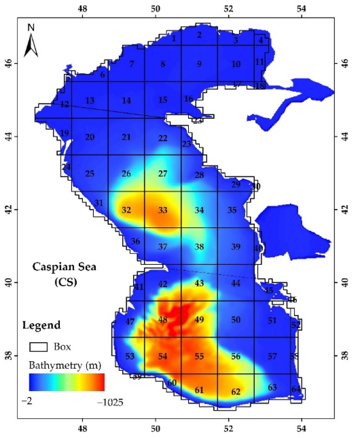
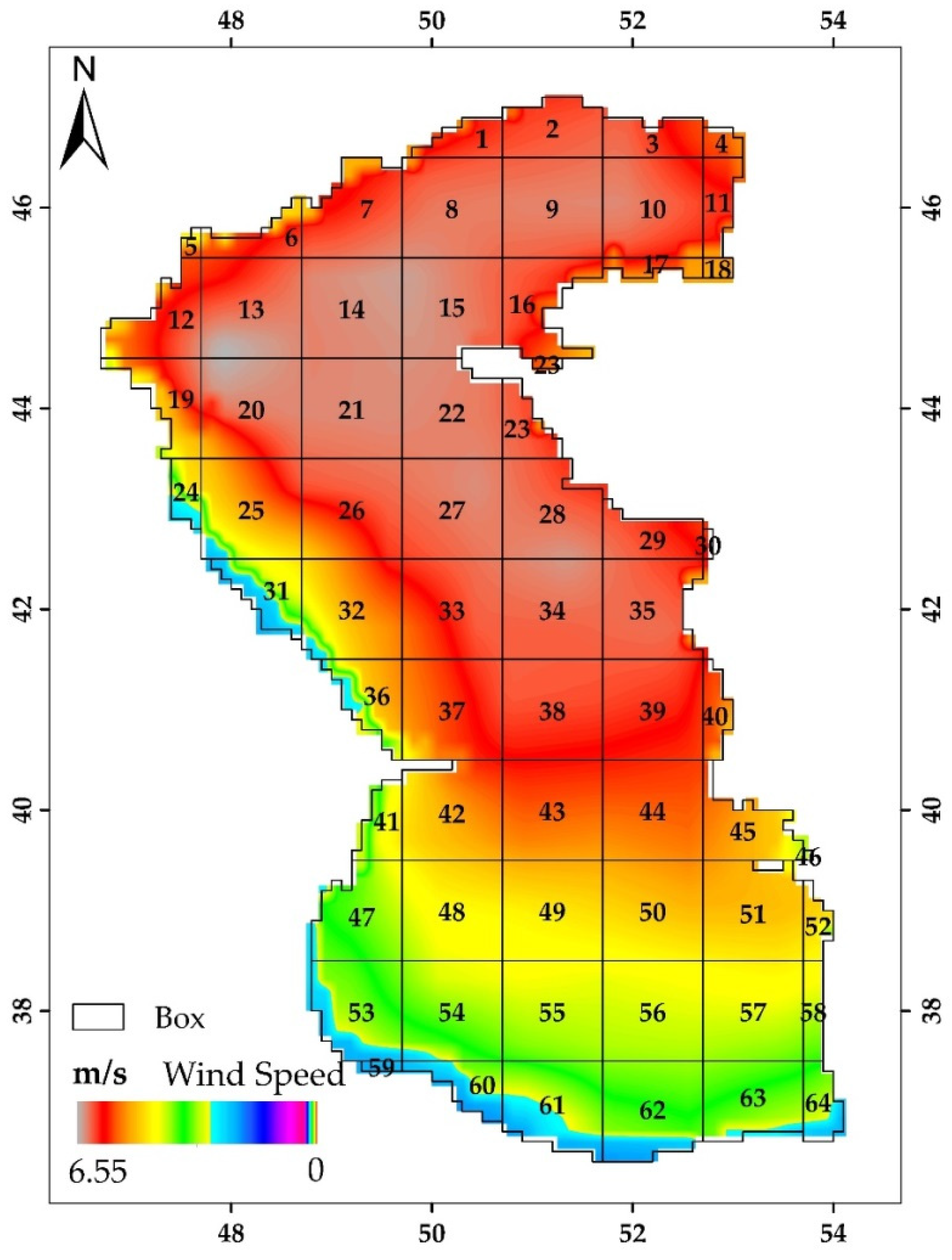
2.1. Study Area
2.2. Data Lake
2.3. Wind Power Density
2.4. Time Series
Mann–Kendall Trend Test
3. Results
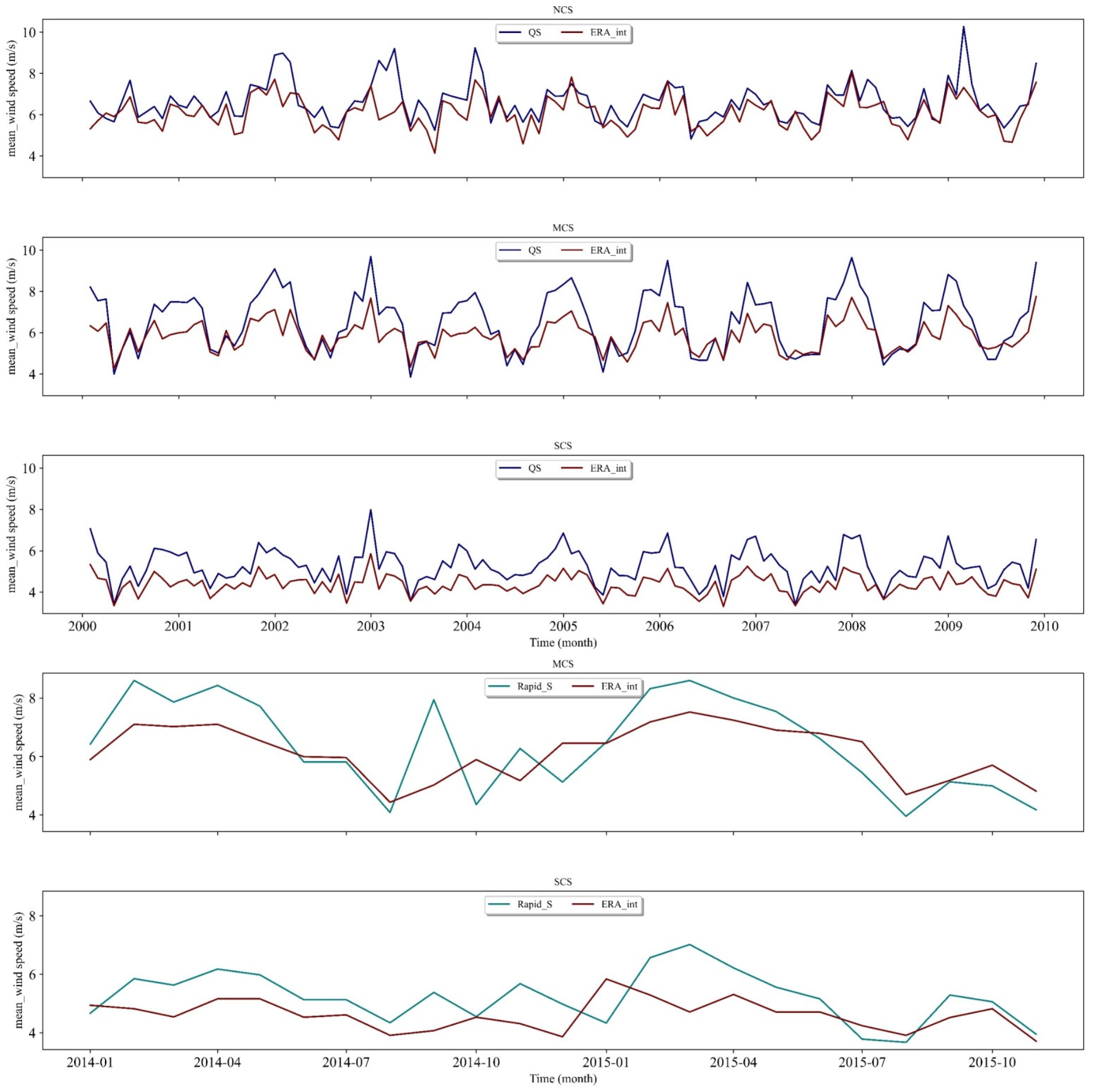
3.1. Wind Data Accuracy Evaluation
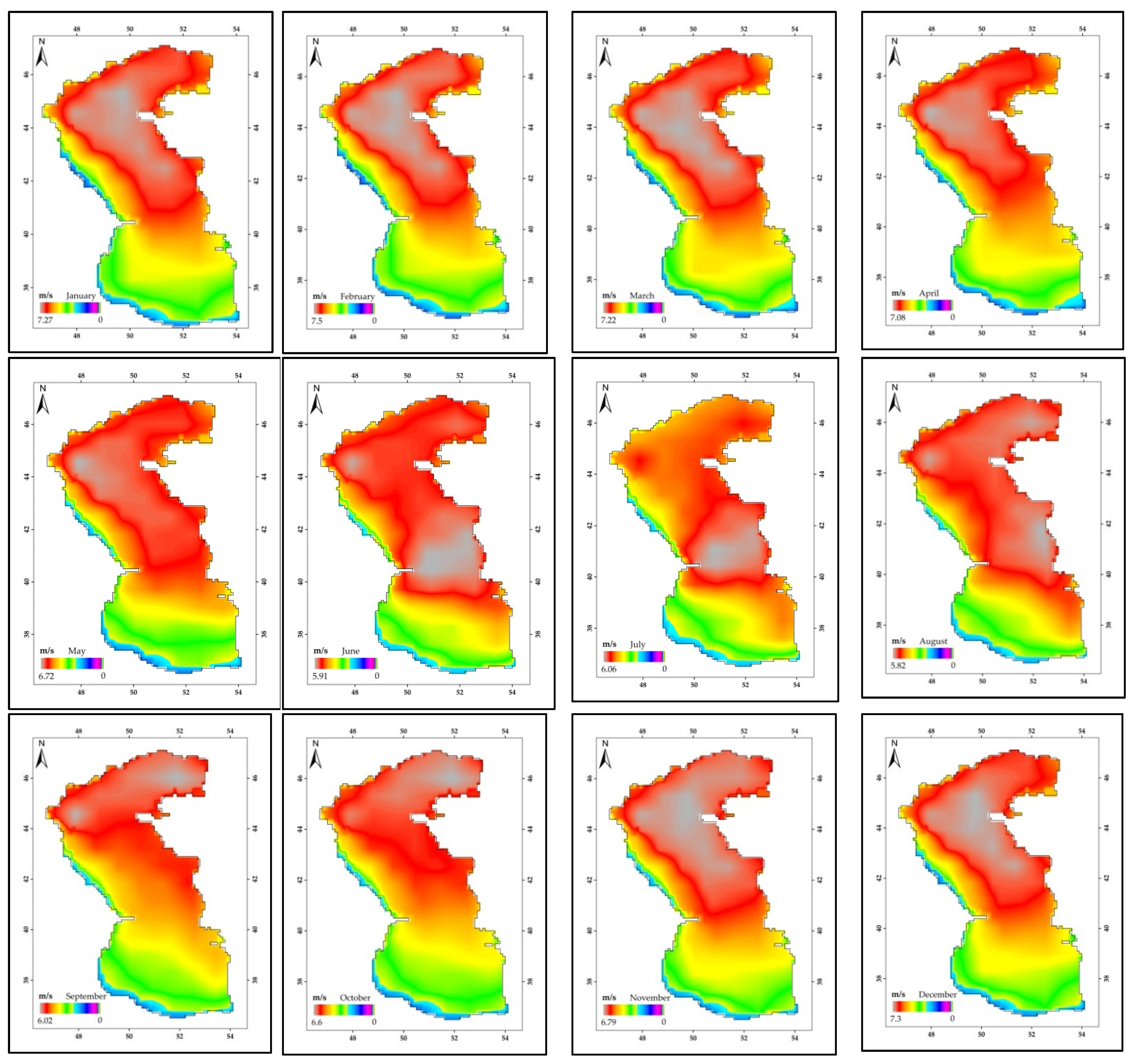
3.2. Wind Speed and Indicators
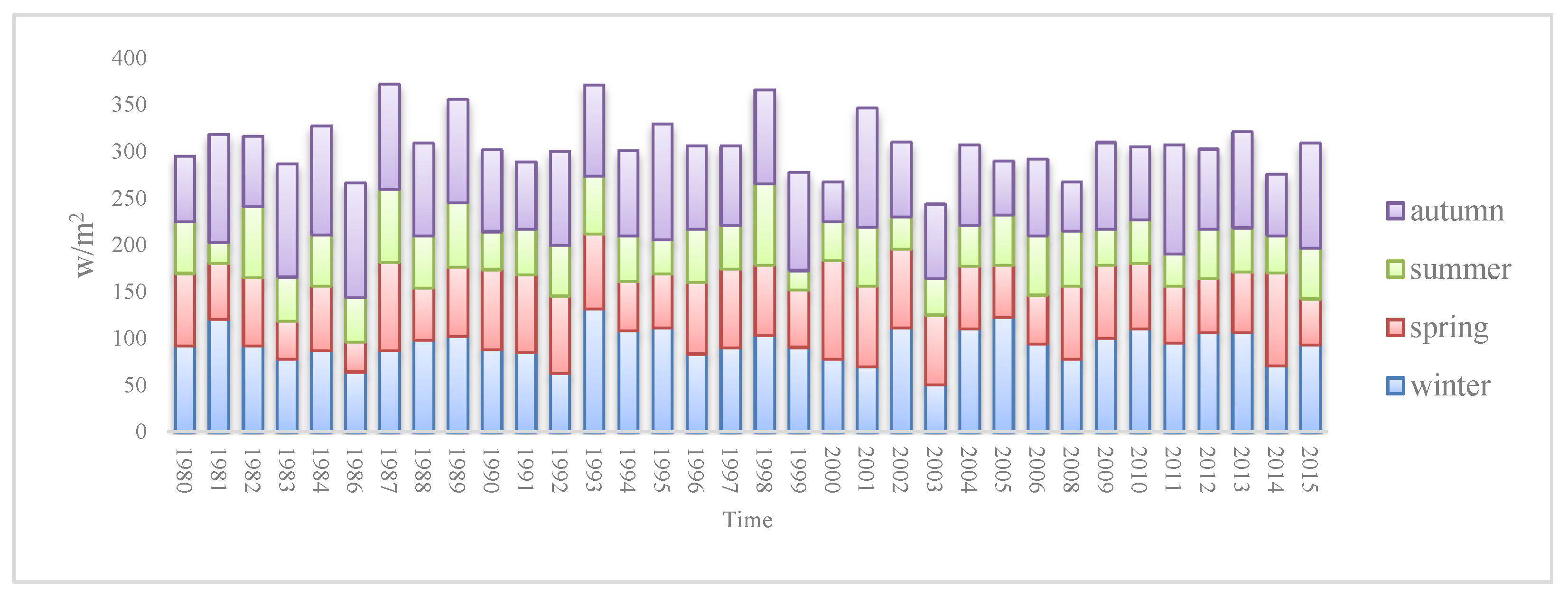
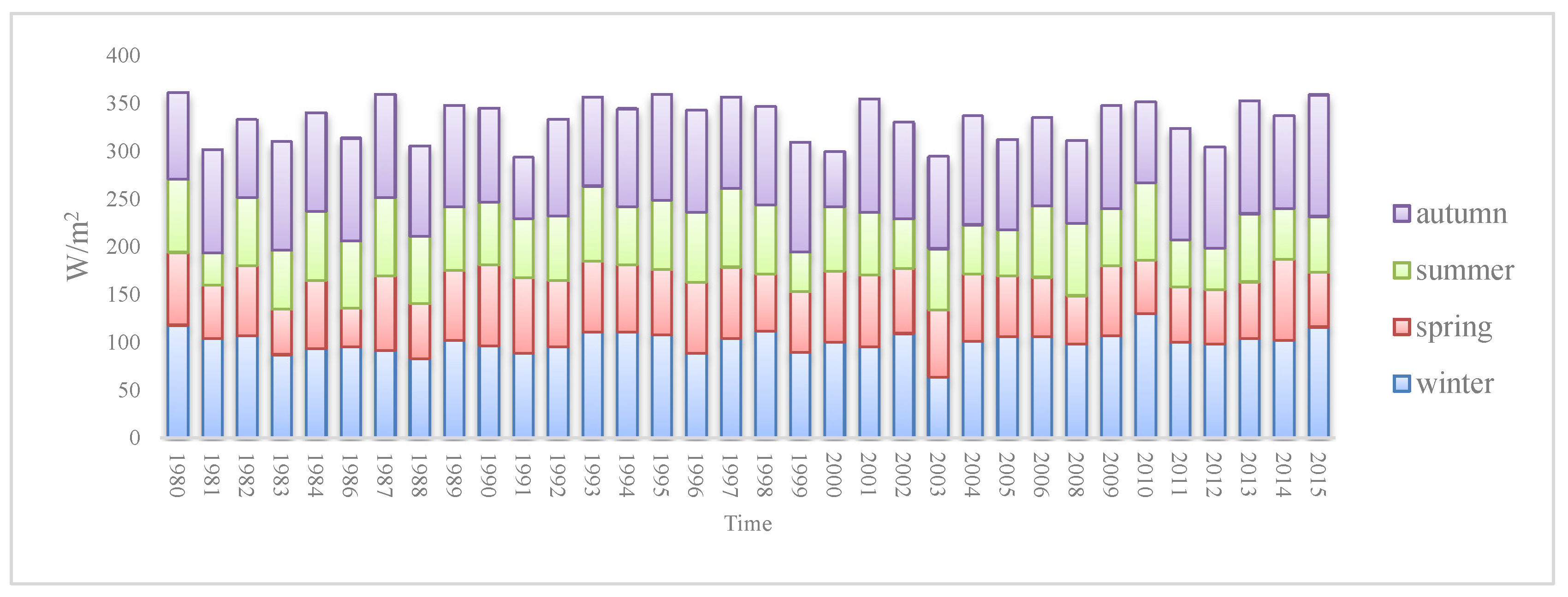
3.3. Wind Power Density
3.4. Analysis of the Interannual Variability Trends
4. Discussion
5. Conclusions
Author Contributions
Funding
Data Availability Statement
Acknowledgments
Conflicts of Interest
References
- Barbier, E.B. Marine ecosystem services. Curr. Biol. 2017, 27, R507–R510. [Google Scholar] [CrossRef] [PubMed]
- Busch, M.; Gee, K.; Burkhard, B.; Lange, M.; Stelljes, N. Conceptualizing the link between marine ecosystem services and human well-being: The case of offshore wind farming. Int. J. Biodivers. Sci. Ecosyst. Serv. Manag. 2011, 7, 190–203. [Google Scholar] [CrossRef]
- Fisher, B.; Turner, R.K.; Morling, P. Defining and classifying ecosystem services for decision making. Ecol. Econ. 2009, 68, 643–653. [Google Scholar] [CrossRef]
- Fisher, B.; Turner, R.K. Ecosystem services: Classification for valuation. Biol. Conserv. 2008, 141, 1167–1169. [Google Scholar] [CrossRef]
- Lee, J.; Backwell, B.; Clarke, E.; Williams, R.; Liang, W.; Fang, E.; Ladwa, R.; Muchiri, W.; Fiestas, R.; Qiao, L.; et al. Global Wind Report 2022; GWEC: Brussels, Belgium, 2022; p. 158. [Google Scholar]
- Mostafaeipour, A. Feasibility study of offshore wind turbine installation in Iran compared with the world. Renew. Sustain. Energy Rev. 2010, 14, 1722–1743. [Google Scholar] [CrossRef]
- Rabbani, R.; Zeeshan, M. Exploring the suitability of MERRA-2 reanalysis data for wind energy estimation, analysis of wind characteristics and energy potential assessment for selected sites in Pakistan. Renew. Energy 2020, 154, 1240–1251. [Google Scholar] [CrossRef]
- Olauson, J. ERA5: The new champion of wind power modelling? Renew. Energy 2018, 126, 322–331. [Google Scholar] [CrossRef]
- Osinowo, A.A.; Lin, X.; Zhao, D.; Zheng, K. On the wind energy resource and its trend in the East China Sea. J. Renew. Energy 2017, 2017, 9643130. [Google Scholar] [CrossRef]
- Cannon, D.J.; Brayshaw, D.J.; Methven, J.; Coker, P.J.; Lenaghan, D. Using reanalysis data to quantify extreme wind power generation statistics: A 33 year case study in Great Britain. Renew. Energy 2015, 75, 767–778. [Google Scholar] [CrossRef]
- Kubik, M.; Brayshaw, D.J.; Coker, P.J.; Barlow, J.F. Exploring the role of reanalysis data in simulating regional wind generation variability over Northern Ireland. Renew. Energy 2013, 57, 558–561. [Google Scholar] [CrossRef]
- Capps, S.B.; Zender, C.S. Estimated global ocean wind power potential from QuikSCAT observations, accounting for turbine characteristics and siting. J. Geophys. Res. Atmos. 2010, 115. [Google Scholar] [CrossRef]
- Pimenta, F.; Kempton, W.; Garvine, R. Combining meteorological stations and satellite data to evaluate the offshore wind power resource of Southeastern Brazil. Renew. Energy 2008, 33, 2375–2387. [Google Scholar] [CrossRef]
- Signell, R.P.; Carniel, S.; Cavaleri, L.; Chiggiato, J.; Doyle, J.D.; Pullen, J.; Sclavo, M. Assessment of wind quality for oceanographic modelling in semi-enclosed basins. J. Mar. Syst. 2005, 53, 217–233. [Google Scholar] [CrossRef]
- Lebedev, S.A.; Kostianoy, A.G. Satellite altimetry of the Caspian Sea. Sea Mosc. 2005, 366, 113–120. [Google Scholar]
- Lebedev, S.A.; Kostianoy, A.G. Integrated use of satellite altimetry in the investigation of the meteorological, hydrological, and hydrodynamic regime of the Caspian Sea. TAO: Terr. Atmos. Ocean. Sci. 2008, 19, 7. [Google Scholar] [CrossRef]
- Zonn, I.S.; Kosarev, A.N.; Glantz, M.H.; Kostianoy, A.G. The Caspian Sea Encyclopedia; Springer: Berlin/Heidelberg, Germany, 2010. [Google Scholar]
- Melnikov, V.; Zatsepin, A.; Kostianoy, A.G. Hydrophysical Polygon on the Black Sea; Russian State Oceanographic Institute: Moscow, Russia, 2011; Volume 213, pp. 264–278. [Google Scholar]
- Hadadpour, S.; Moshfeghi, H.; Jabbari, E.; Kamranzad, B. Wave hindcasting in Anzali, Caspian Sea: A hybrid approach. J. Coast. Res. 2013, 65, 237–242. [Google Scholar] [CrossRef]
- Grinevetsky, S.R.; Zonn, I.S.; Zhiltsov, S.S.; Kosarev, A.N.; Kostianoy, A.G. The Black Sea Encyclopedia; Springer: Berlin/Heidelberg, Germany, 2015. [Google Scholar]
- Evstigneev, V.; Naumova, V.; Voskresenskaya, E.; Evstigneev, M.; Lyubarets, E. Wind-Wave Conditions of the Coastal Zone of the Azov-Black Sea Region; Institute of Natural and Technical Systems: Sevastopol, Crimea, 2017. [Google Scholar]
- Kostianaia, E.A.; Serykh, I.V.; Kostianoy, A.G.; Lebedev, S.A.; Akhsalba, A.K. Climate Changes of the Wind Module in the Region of the Eastern Coast of the Black Sea. Vestn. Tver State Univ. Ser. Geogr. Geoecol. 2018, 3, 79–98. [Google Scholar]
- Serykh, I.; Kostianoy, A. The links of climate change in the Caspian Sea to the Atlantic and Pacific Oceans. Russ. Meteorol. Hydrol. 2020, 45, 430–437. [Google Scholar] [CrossRef]
- Kostianaia, E.A.; Kostianoy, A.G. Regional Climate Change Impact on Coastal Tourism: A Case Study for the Black Sea Coast of Russia. Hydrology 2021, 8, 133. [Google Scholar] [CrossRef]
- Bogdanovich, Y.; Lipka, O.N.; Krylenko, M.V.; Andreeva, A.P.; Dobrolyubova, K.O. Climate threats in the North-West Caucasus Black Sea coast: Modern trends. Fundam. Appl. Climatol. 2021, 7, 44–70. [Google Scholar] [CrossRef]
- Rusu, E. Wind climate scenarios in the Black Sea basin until the end of the 21st century. Rom. J. Tech. Sciences. Appl. Mechanics. 2021, 66, 181–204. [Google Scholar]
- Manzano-Agugliaro, F.; Alcayde, A.; Montoya, F.G.; Zapata-Sierra, A.; Gil, C. Scientific production of renewable energies worldwide: An overview. Renew. Sustain. Energy Rev. 2013, 18, 134–143. [Google Scholar] [CrossRef]
- Kerimov, R.; Ismailova, Z.; Rahmanov, N. Modeling of wind power producing in Caspian Sea conditions. Int. J. Tech. Phys. Probl. Eng. 2013, 15, 136–142. [Google Scholar]
- Rusu, E.; Onea, F. Evaluation of the wind and wave energy along the Caspian Sea. Energy 2013, 50, 1–14. [Google Scholar] [CrossRef]
- Onea, F.; Rusu, E. Wind energy assessments along the Black Sea basin. Meteorol. Appl. 2014, 21, 316–329. [Google Scholar] [CrossRef]
- Onea, F.; Rusu, E. An evaluation of the wind energy in the North-West of the Black Sea. Int. J. Green Energy 2014, 11, 465–487. [Google Scholar] [CrossRef]
- Rahmanov, N.; Kerimov, R.; Gurbanov, E. Assessing the wind potential of Caspian Sea region for covering demand in neighboring countries and reducing of carbon emission. In Proceedings of the 2nd International Symposium on Energy Challenges & Mechanics, Aberdeen, UK, 18–20 August 2014. [Google Scholar]
- Onea, F.; Raileanu, A.; Rusu, E. Evaluation of the wind energy potential in the coastal environment of two enclosed seas. Adv. Meteorol. 2015, 2015, 808617. [Google Scholar] [CrossRef]
- Amirinia, G.; Kamranzad, B.; Mafi, S. Wind and wave energy potential in southern Caspian Sea using uncertainty analysis. Energy 2017, 120, 332–345. [Google Scholar] [CrossRef]
- Terziev, S.; Kosarev, A.; Kerimov, A. Hydrometeorology and hydrochemistry of seas. Vol. 6, the Caspian Sea, No. 1. Hydrometeorological Conditions. Leningr. Gidrometeoizdat 1992, 6, 358p. (In Russian) [Google Scholar]
- Mazaheri, S.; Kamranzad, B.; Hajivalie, F. Modification of 32 years ECMWF wind field using QuikSCAT data for wave hindcasting in Iranian Seas. J. Coast. Res. 2013, 65, 344–349. [Google Scholar] [CrossRef]
- Kamranzad, B.; Etemad-Shahidi, A.; Chegini, V.; Hadadpour, S. Assessment of CGCM 3.1 wind field in the Persian Gulf. J. Coast. Res. 2013, 65, 249–253. [Google Scholar] [CrossRef]
- Kramer, H.J. QuikSCAT. Available online: https://www.eoportal.org/satellite-missions/quikscat#seawinds (accessed on 21 November 2022).
- Hoffmann, L.; Spang, R. An assessment of tropopause characteristics of the ERA5 and ERA-Interim meteorological reanalyses. Atmos. Chem. Phys. 2022, 22, 4019–4046. [Google Scholar] [CrossRef]
- Dee, D.P.; Uppala, S.M.; Simmons, A.J.; Berrisford, P.; Poli, P.; Kobayashi, S.; Andrae, U.; Balmaseda, M.; Balsamo, G.; Bauer, P. The ERA-Interim reanalysis: Configuration and performance of the data assimilation system. Q. J. R. Meteorol. Soc. 2011, 137, 553–597. [Google Scholar] [CrossRef]
- Kalam Azad, A.; Golam Rasul, M.; Yusaf, T. Statistical Diagnosis of the Best Weibull Methods for Wind Power Assessment for Agricultural Applications. Energies 2014, 7, 3056–3085. [Google Scholar] [CrossRef]
- Twidell, J.; Gaudiosi, G. Offshore Wind Power; Multi-Science Publishing Company: Brentwood, UK, 2009; Volume 425. [Google Scholar]
- Lai, C.-D. Generalized Weibull Distributions. In Generalized Weibull Distributions; Springer: Berlin/Heidelberg, Germany, 2014; pp. 23–75. [Google Scholar]
- Bidaoui, H.; El Abbassi, I.; El Bouardi, A.; Darcherif, A. Wind speed data analysis using Weibull and Rayleigh distribution functions, case study: Five cities northern Morocco. Procedia Manuf. 2019, 32, 786–793. [Google Scholar] [CrossRef]
- Pishgar-Komleh, S.; Keyhani, A.; Sefeedpari, P. Wind speed and power density analysis based on Weibull and Rayleigh distributions (a case study: Firouzkooh county of Iran). Renew. Sustain. Energy Rev. 2015, 42, 313–322. [Google Scholar] [CrossRef]
- Kollu, R.; Rayapudi, S.R.; Narasimham, S.; Pakkurthi, K.M. Mixture probability distribution functions to model wind speed distributions. Int. J. Energy Environ. Eng. 2012, 3, 1–10. [Google Scholar] [CrossRef]
- Pal, M.; Ali, M.M.; Woo, J. Exponentiated weibull distribution. Statistica 2006, 66, 139–147. [Google Scholar]
- Ahmadi, B.; Gholamalifard, M.; Kutser, T.; Vignudelli, S.; Kostianoy, A. Spatio-Temporal Variability in Bio-Optical Properties of the Southern Caspian Sea: A Historic Analysis of Ocean Color Data. Remote Sens. 2020, 12, 3975. [Google Scholar] [CrossRef]
- Neeti, N.; Eastman, J.R. A contextual mann-kendall approach for the assessment of trend significance in image time series. Trans. GIS 2011, 15, 599–611. [Google Scholar] [CrossRef]
- Ruti, P.M.; Marullo, S.; d’Ortenzio, F.; Tremant, M. Comparison of analyzed and measured wind speeds in the perspective of oceanic simulations over the Mediterranean basin: Analyses, QuikSCAT and buoy data. J. Mar. Syst. 2008, 70, 33–48. [Google Scholar] [CrossRef]
- Golshani, A.A.; Taebi, S. Evaluation of wind vectors observed by quikscat/seawinds using synoptic and atmospheric models data in iranian adjacant seas. J. Mar. Eng. 2009, 4, 47–63. [Google Scholar]
- Zhiltsov, S.S.; Zonn, I.S.; Kostianoy, A.G.; Semenov, A.V. The Caspian Sea Region. Subjects of the Caspian Littoral Countries: Geography, Resources, Economics; Witte Moscow University: Moscow, Russia, 2019; Volume 3, 200p. [Google Scholar]
- Zonn, I.S.; Kostianoy, A.G.; Zhiltsov, S.S.; Semenov, A.V. The Caspian Sea Region. The Caspian Sea and the History of Its Exploration; Witte Moscow University: Moscow, Russia, 2019; Volume 2, 312p. [Google Scholar]
- Fore, A.G.; Stiles, B.W.; Chau, A.H.; Williams, B.A.; Dunbar, R.S.; Rodríguez, E. Point-wise wind retrieval and ambiguity removal improvements for the QuikSCAT climatological data set. IEEE Trans. Geosci. Remote Sens. 2013, 52, 51–59. [Google Scholar] [CrossRef]
- Lavrova, O.Y.; Ginzburg, A.I.; Kostianoy, A.G.; Bocharova, T.Y. Interannual variability of ice cover in the Caspian Sea. J. Hydrol. 2022, 17, 100145. [Google Scholar] [CrossRef]
- Lavrova, O.Y.; Kostianoy, A.G.; Mityagina, M.I.; Strochkov, A.Y.; Bocharova, T.Y. Remote sensing of sea ice in the Caspian Sea. In Proceedings of the Remote Sensing of the Ocean, Sea Ice, Coastal Waters, and Large Water Regions, Strasbourg, France, 9–12 September 2019; pp. 193–204. [Google Scholar]
- González, J.S.; Payán, M.B.; Santos, J.M.R.; Rodríguez, Á.G.G. Optimal Micro-Siting of Weathervaning Floating Wind Turbines. Energies 2021, 14, 886. [Google Scholar] [CrossRef]


| Part | Satellite | Mean (m/s) | SD (m/s) | MIN (m/s) | MAX (m/s) | CC (m/s) |
|---|---|---|---|---|---|---|
| Northern Caspian | QuikSCAT | 5.26 | 0.48 | 3.08 | 8.93 | 0.75 |
| ERA-Interim | 4.37 | 0.43 | 2.7 | 5.82 | ||
| Middle Caspian | QuikSCAT | 6.56 | 0.6 | 4.29 | 8.85 | 0.83 |
| ERA-Interim | 5.84 | 0.53 | 4.13 | 6.69 | ||
| Southern Caspian | QuikSCAT | 6.45 | 0.6 | 0 | 10.35 | 0.59 |
| ERA-Interim | 6.09 | 0.55 | 5.35 | 6.65 |
| Part | Satellite | Mean (m/s) | SD (m/s) | MIN (m/s) | MAX (m/s) | CC (m/s) |
|---|---|---|---|---|---|---|
| Middle Caspian | RapidSCAT | 6.41 | 1.54 | 3.97 | 7.52 | 0.67 |
| ERA-Interim | 6.15 | 0.89 | 4.43 | 5.6 | ||
| Southern Caspian | RapidSCAT | 5.22 | 0.85 | 3.67 | 7.2 | 0.37 |
| ERA-Interim | 4.61 | 0.51 | 3.71 | 5.84 |
Publisher’s Note: MDPI stays neutral with regard to jurisdictional claims in published maps and institutional affiliations. |
© 2022 by the authors. Licensee MDPI, Basel, Switzerland. This article is an open access article distributed under the terms and conditions of the Creative Commons Attribution (CC BY) license (https://creativecommons.org/licenses/by/4.0/).
Share and Cite
Rahimi, M.; Gholamalifard, M.; Rashidi, A.; Ahmadi, B.; Kostianoy, A.G.; Semenov, A.V. Spatio-Temporal Variability of Wind Energy in the Caspian Sea: An Ecosystem Service Modeling Approach. Remote Sens. 2022, 14, 6263. https://doi.org/10.3390/rs14246263
Rahimi M, Gholamalifard M, Rashidi A, Ahmadi B, Kostianoy AG, Semenov AV. Spatio-Temporal Variability of Wind Energy in the Caspian Sea: An Ecosystem Service Modeling Approach. Remote Sensing. 2022; 14(24):6263. https://doi.org/10.3390/rs14246263
Chicago/Turabian StyleRahimi, Milad, Mehdi Gholamalifard, Akbar Rashidi, Bonyad Ahmadi, Andrey G. Kostianoy, and Aleksander V. Semenov. 2022. "Spatio-Temporal Variability of Wind Energy in the Caspian Sea: An Ecosystem Service Modeling Approach" Remote Sensing 14, no. 24: 6263. https://doi.org/10.3390/rs14246263
APA StyleRahimi, M., Gholamalifard, M., Rashidi, A., Ahmadi, B., Kostianoy, A. G., & Semenov, A. V. (2022). Spatio-Temporal Variability of Wind Energy in the Caspian Sea: An Ecosystem Service Modeling Approach. Remote Sensing, 14(24), 6263. https://doi.org/10.3390/rs14246263